The Banff Challenge: Statistical Detection of a Noisy Signal

Abstract

Particle physics experiments such as those run in the Large Hadron Collider result in huge quantities of data, which are boiled down to a few numbers from which it is hoped that a signal will be detected. We discuss a simple probability model for this and derive frequentist and noninformative Bayesian procedures for inference about the signal. Both are highly accurate in realistic cases, with the frequentist procedure having the edge for interval estimation, and the Bayesian procedure yielding slightly better point estimates. We also argue that the significance, or $p$-value, function based on the modified likelihood root provides a comprehensive presentation of the information in the data and should be used for inference.

and

Bayesian inference, higher-order asymptotics, Large Hadron Collider, likelihood, noninformative prior, orthogonal parameter, particle physics, Poisson distribution, signal detection

1 Introduction

Particle physics experiments such as those conducted in the Large Hadron Collider entail the detection of a signal in the presence of background noise. This essentially statistical topic has been discussed intensively in the recent literature (Mandelkern (2002), Fraser, Reid and Wong (2004), and the references therein) and at a series of meetings involving statisticians and physicists; see Lyons (2008) for more details and further references. One key issue is the setting of confidence limits on the underlying signal, based on data from independent observation channels.

In the simplest version of the problem there is just one channel, the observation from which is the number of times a particular event in a particle accelerator has been observed. This is supposed to have a Poisson distribution with mean $\gamma\psi+\beta$, where the positive known constants $\beta$ and $\gamma$ represent respectively a background rate at which the event occurs and the efficiency of the measurement device. There is a substantial physical literature about inference for the focus of interest, the unknown parameter $\psi$. Typically frequentist inference is preferred to Bayesian approaches, but this is the subject of a lively debate among the scientists involved. In order to compare properties of various procedures for inference about $\psi$, it was decided at the workshop on Statistical Inference Problems in High Energy Physics and Astronomy held at the Banff International Research Station in 2006 that one participant would create artificial data that should mimic those that might arise when the Large Hadron Collider is running, and that other participants would attempt to set confidence limits for the known underlying signal. Thus was the Banff Challenge (http://newton.hep.upenn.edu/~heinrich/birs/) born.

For a single channel the challenge may be stated as follows: the available data $y_{1},y_{2},y_{3}$ are assumed to be realizations of independent Poisson random variables with means $\gamma\psi+\beta,\beta t,\gamma u$, where $t,u$ are known and the parameters $\psi,\beta,\gamma$ are unknown. This expands the formulation above to allow for uncertainty about the values of the background $\beta$ and the efficiency $\gamma$, which are supposed to be estimable from subsidiary experiments of known lengths $t$ and $u$. The goal is to summarize the evidence concerning $\psi$, large estimates of which will suggest presence of the signal. The parameters $\beta$ and $\gamma$ are necessary for realism, but their values are only of concern to the extent that they impinge on inference for $\psi$.

This is a highly idealized version of one of many statistical problems that will arise in dealing with data from the Large Hadron Collider. The model is very simple, but important inferential issues arise nonetheless: how is evidence about the value of $\psi$ best summarized? How should one deal with the nuisance parameters $\beta,\gamma$? This second issue is even more critical in the case of multiple channels, where the number of nuisance parameters is much larger. Below we follow Fraser, Reid and Wong (2004) in arguing that the evidence concerning $\psi$ is best summarized through a so-called significance function, and in Section 2 describe the general construction of significance functions that yield highly accurate frequentist inferences even with many nuisance parameters; such a significance function is equivalent to a set of confidence intervals at various levels. In Section 3 we give results for the Poisson model for the two cases laid out in the Banff Challenge, with one channel and with ten channels.

Statisticians are in broad agreement that the likelihood function is central to parametric inference. Bayesian inference uses the likelihood to update prior information to give a posterior probability density that summarises what it is reasonable to believe about the parameters in light of the data (Jeffreys (1961), O’Hagan and Forster (2004)). This approach is attractive and widely used in applications, but scientists with different priors may arrive at different conclusions based on the same data. One might argue that this is inevitable given the varied points of view held within any scientific community, but this lack of uniqueness is awkward when an objective statement is sought. One way to unite this multiplicity of possible posterior beliefs is to base inference on a noninformative prior, which we discuss in Section 4 for the Poisson model described above.

One aspect we discuss only peripherally is the choice of the Poisson distribution to represent the variation of the observed events. Statisticians typically regard a model as one of many possibilities, whereas physicists tend to argue from first principles and the known properties of the systems that they study toward a strong belief that certain models, such as the Poisson law used here, are correct. Under the Banff Challenge the Poissonness of the observations is taken as given.

2 Likelihood and Significance

There are many published accounts of modern likelihood theory. The outline below is based on Brazzale, Davison and Reid (2007), wherein further references may be found.

We consider a probability density function $f(y;\psi,\break\lambda)$ that depends on two parameters. The interest parameter $\psi$ is the focus of the investigation; one may wish to test whether it has a specific value $\psi_{0}$, or to produce a confidence interval for the true but unknown value of $\psi$. Often $\psi$ is scalar, as here: $\psi$ represents the signal central to our enquiry. The nuisance parameter $\lambda$ is not of direct interest, but must be included for the model to be realistic. In the single-channel case the vector $\lambda=(\beta,\gamma)$ represents the background signal and measurement efficiency. Let $\theta=(\psi,\lambda)$ denote the entire parameter vector.

The log likelihood function is defined as $\ell(\theta)=\log f(y;\theta)$. The maximum likelihood estimator $\widehat{\theta}$ satisfies $\ell(\widehat{\theta})\geq\ell(\theta)$ for all $\theta$ lying in the parameter space $\Omega_{\theta}$, which we take to be an open subset of $\mathbb{R}^{d}$. We suppose that $\psi$ may take values in the interval $(\psi_{-},\psi_{+})$, where one or both of the limits $\psi_{-},\psi_{+}$ may be infinite. A natural summary of the support for $\psi$ provided by the combination of model and data is the profile log likelihood

$$\ell_{\mathrm{p}}(\psi)=\ell(\widehat{\theta}_{\psi})=\ell(\psi,\widehat{\lambda}_{\psi})=\max_{\lambda}\ell(\psi,\lambda),$$

where $\widehat{\lambda}_{\psi}$ is the value of $\lambda$ that maximizes the log likelihood for fixed $\psi$.

Under regularity conditions on $f$ under which a random sample of size $n$ is generated from $f(y;\theta_{0})$, the estimator $\widehat{\theta}$ has an approximate normal distribution with mean $\theta_{0}$ and variance matrix $j(\widehat{\theta})^{-1}$, where $j(\theta)=-\partial^{2}\ell(\theta)/\partial\theta\,\partial\theta^{\mathrm{T}}$ is the observed information matrix. This result can be used as the basis of confidence intervals for $\psi_{0}$, based on the limiting standard normal, $\mathcal{N}(0,1)$, distribution of the Wald pivot $t(\psi_{0})=j_{\mathrm{p}}(\widehat{\psi})^{1/2}(\widehat{\psi}-\psi_{0})$, where

$$j_{\mathrm{p}}(\psi)=-{\partial^{2}\ell_{\mathrm{p}}(\psi)\over\partial\psi^{2}}={|j(\psi,\widehat{\lambda}_{\psi})|\over|j_{\lambda\lambda}(\psi,\widehat{\lambda}_{\psi})|},$$

$|\cdot|$ indicates determinant, and $j_{\lambda\lambda}(\theta)$ denotes the $(\lambda,\lambda)$ corner of the observed information matrix. In many ways a preferable basis for confidence intervals is the likelihood root

$$r(\psi)=\operatorname{sign}(\widehat{\psi}-\psi)[2\{\ell_{\mathrm{p}}(\widehat{\theta})-\ell_{\mathrm{p}}(\widehat{\theta}_{\psi})\}]^{1/2},$$

which may also be treated as an $\mathcal{N}(0,1)$ variable. If it is required to test the hypothesis that $\psi=\psi_{0}$ against the one-sided hypothesis that $\psi>\psi_{0}$, then the quantities $1-\Phi\{r(\psi_{0})\}$ and $1-\Phi\{t(\psi_{0})\}$ are treated as significance probabilities, also known as $p$-values, small values of which will cast doubt on the belief that $\psi=\psi_{0}$. Throughout the paper $\Phi$ represents the cumulative probability function of the standard normal distribution.

The monotonic decreasing function $\Phi\{r(\psi)\}$ is an example of a significance function, from which we may draw inferences about $\psi$. An approximate lower confidence bound $\psi_{\alpha}$ for $\psi_{0}$ is the solution to the equation $\Phi\{r(\psi)\}=1-\alpha$; the confidence interval $(\psi_{\alpha},\psi_{+})$ should contain $\psi_{0}$ with probability $1-\alpha$. An approximate upper bound $\psi_{1-\alpha}$ is obtained by solution of $\Phi\{r(\psi)\}=\alpha$, giving confidence interval $(\psi_{-},\psi_{1-\alpha})$, and the two-sided interval $(\psi_{\alpha},\psi_{1-\alpha})$ will contain $\psi_{0}$ with probability approximately $(1-2\alpha)$. Using these so-called first-order approximations, these one-sided intervals in fact contain $\psi_{0}$ with probability $1-\alpha+\mathcal{O}(n^{-1/2})$, while the two-sided interval contains $\psi_{0}$ with probability $(1-2\alpha)+\mathcal{O}(n^{-1})$. Significance functions may be based on the Wald pivot $t(\psi)$ or on related quantities involving the log likelihood derivative $\partial\ell/\partial\psi$, which also have approximate $\mathcal{N}(0,1)$ distributions for large $n$, but the intervals based on $r(\psi)$ are preferable because they always yield confidence sets that are subsets of $(\psi_{-},\psi_{+})$. Further, they are invariant to invertible interest-preserving reparametrization, of the form $(\psi,\lambda)\mapsto(g(\psi),h(\lambda,\psi))$: if $\mathcaligr{I}$ is a confidence interval for $\psi$ in the original parametrization, then $g(\mathcaligr{I})$ is the corresponding interval in the new parametrization; this property is not possessed by intervals based on the Wald pivot, for example.

A large body of literature on higher-order parametric asymptotics, both Bayesian and frequentist, has converged on a few key formulae that are useful for inference. There are numerous derivations of these formulae in different cases, for example by Laplace approximation to posterior densities or by saddlepoint approximation to conditional densities; see Reid (2003) or Davison (2003, Sections 11.3.1, 12.3.3). Fuller accounts are given by Brazzale, Davison and Reid (2007), Severini (2000), Pace and Salvan (1997) and Barndorff-Nielsen and Cox (1994). Perhaps the most practicable route to these improved inferences is through significance functions based on the modified likelihood root

$$r^{*}(\psi)=r(\psi)+{1\over r(\psi)}\log\biggl{\{}{q(\psi)\over r(\psi)}\biggr{\}},$$ (1)

where

$$\qquad q(\psi)={|\varphi(\widehat{\theta})-\varphi(\widehat{\theta}_{\psi})\varphi_{\lambda}(\widehat{\theta}_{\psi})|\over|\varphi_{\theta}(\widehat{\theta})|}\biggl{\{}{|j(\widehat{\theta})|\over|j_{\lambda\lambda}(\widehat{\theta}_{\psi})|}\biggr{\}}^{1/2}$$ (2)

is determined by a local exponential family approximation whose canonical parameter $\varphi(\theta)$ is described below, and $\varphi_{\theta}$ denotes the $d\times d$ matrix $\partial\varphi/\partial\theta^{\mathrm{T}}$ of partial derivatives. The numerator of the first term of (2) is the determinant of a $d\times d$ matrix whose first column is $\varphi(\widehat{\theta})-\varphi(\widehat{\theta}_{\psi})$ and whose remaining columns are $\varphi_{\lambda}(\widehat{\theta}_{\psi})$. For continuous variables, one-sided confidence intervals based on the significance function $\Phi\{(r^{*}(\psi)\}$ have coverage error $\mathcal{O}(n^{-3/2})$ rather than $\mathcal{O}(n^{-1/2})$.

For a sample of independent continuous observations $y_{1},\ldots,y_{n}$, we define

$$\varphi(\theta)^{\mathrm{T}}=\sum_{k=1}^{n}{\partial\ell(\theta;y)\over\partial y_{k}}\bigg{|}_{y=y^{0}}V_{k},$$

where $y^{0}$ denotes the observed data, and $V_{1},\ldots,V_{n}$ is a set of $1\times d$ vectors that depend on the observed data alone. If the observations are discrete, then the theoretical accuracy of the approximations isreduced to $\mathcal{O}(n^{-1})$, and the interpretation ofsignificance functions such as $\Phi\{r^{*}(\theta)\}$ changesslightly. In the discrete setting of this paper we take (Davison, Fraser and Reid, 2006)

$$V_{k}={\partial\mathrm{E}(Y_{k};\theta)\over\partial\theta^{\mathrm{T}}}\bigg{|}_{\theta=\widehat{\theta}},$$ (3)

where $\mathrm{E}$ denotes expectation. An important special case is that of a log likelihood with independent contributions of curved exponential family form,

$$\ell(\theta)=\sum_{k=1}^{n}\{\alpha_{k}(\theta)y_{k}-c_{k}(\theta)\},$$ (4)

where $\alpha_{k}(\theta)y_{k}$ denotes scalar product. In this case

$$\varphi(\theta)^{\mathrm{T}}=\sum_{k=1}^{n}\alpha_{k}(\theta)V_{k}.$$ (5)

Inference using (1) is easily performed. If functions are available to compute $\ell(\theta)$ and $\varphi(\theta)$, then the maximizations needed to obtain $\widehat{\theta}$ and $\widehat{\theta}_{\psi}$ and the differentiation needed to compute (2) may be performed numerically.

Inferences based on (1) are invariant to addition to the log likelihood of quantities dependent only on the data, which lead to affine transformations of $\varphi(\theta)$ by quantities that are parameter independent and which therefore leave (2) unchanged.

As with other uses of approximations in applied mathematics, asymptotic results like those sketched above in which $n\to\infty$ are intended for use with samples whose size is fixed and finite. The key is that some measure of information, which may depend on the parameter values as well as on sample size, becomes large; in the present case information also accumulates as the Poisson means increase. Both general theory and the simulations described below suggest that the higher-order approximations outlined above are highly accurate even when little information is available.

3 Likelihood Inference

3.1 Model Formulation

Under the proposed model, the observation for the $k$th channel is assumed to be a realization of $Y_{k}=(Y_{1k},Y_{2k},Y_{3k})$, where the three components are independent Poisson variables with respective means $(\gamma_{k}\psi+\beta_{k},\beta_{k}t_{k},\gamma_{k}u_{k})$, for $k=1,\ldots,n$. Here $Y_{1k}$ represents the main measurement, $Y_{2k}$ and $Y_{3k}$ are respectively subsidiary background and efficiency measurements, and $t_{k}$ and $u_{k}$ are known positive constants.

The signal parameter $\psi$ is of interest, and $(\beta_{1},\gamma_{1},\break\ldots,\beta_{n},\gamma_{n})$ is treated as a nuisance parameter. In principle the nuisance parameters are positive and $\psi\geq 0$, but it is mathematically reasonable to entertain negative values for $\psi$, provided $\psi>\max_{k}\{-\beta_{k}/\break\gamma_{k}\}$. Below we use this extended parameter space for numerical purposes, but restrict interpretation of the results to the physically meaningful values $\psi\geq 0$, as suggested by Fraser, Reid and Wong (2004).

For computational purposes we take $\lambda=(\lambda_{11},\lambda_{21},\break\ldots,\lambda_{1n},\lambda_{2n})$, with $(\lambda_{1k},\lambda_{2k})=(\log\beta_{k}-\log\gamma_{k},\break\log\beta_{k})$, so that $\exp(\lambda_{1k})>-\psi$ and $\lambda_{2k}\in\mathbb{R}$, $k=1,\ldots,n$. The invariance properties outlined in the previous section imply that inferences on $\psi$ are unaffected by this reparametrization.

The log likelihood function for $\theta=(\psi,\lambda)$ has curved exponential family form (4) with

$$\alpha_{k}(\theta)^{\mathrm{T}} = \{\log(\psi e^{\lambda_{2k}-\lambda_{1k}}+e^{\lambda_{2k}}),$$

$$\hskip 32.6pt\lambda_{2k},(\lambda_{2k}-\lambda_{1k})\},$$

$$y_{k}^{\mathrm{T}} = (y_{1k},y_{2k},y_{3k}),$$

$$c_{k}(\theta) = (\psi+u_{k})e^{\lambda_{2k}-\lambda_{1k}}+(1+t_{k})e^{\lambda_{2k}}.$$

In general, $\widehat{\theta}$ and $\widehat{\theta}_{\psi}$ must be computed numerically. It is convenient to compute $\widehat{\theta}_{\psi}$ first, and then obtain $\widehat{\theta}$ by maximizing the profile log likelihood $\ell(\widehat{\theta}_{\psi})$.

The dimension of the nuisance parameter may be reduced by a conditioning argument that applies to Poisson responses, but for simplicity of exposition we use the Poisson formulation here. The trinomial model that emerges from the conditioning is used below in Section 4.2. Properties of the Poisson model imply that numerical results from the two formulations are identical.

3.2 One Channel

When data from only one channel are available, that is, $n=1$, the log likelihood has full exponential form. The canonical parameter $\varphi(\theta)$ given by (3.1) is then equivalent to (5) in the sense that any affine transformation of the canonical parameter gives the same $q(\psi)$ in (2) and the same inference for $\psi$.

A standard way to summarize the evidence concerning $\psi$ is to present the profile log likelihood $\ell_{\mathrm{p}}(\psi)$ and the significance function $\Phi\{r(\psi)\}$ (Fraser, Reid and Wong (2004)), but, as mentioned above, more accurate inferences are obtained from the modified likelihood root, $r^{*}(\psi)$. As the profile log likelihood equals $-r(\psi)^{2}/2$, the quantity $-r^{*}(\psi)^{2}/2$ can be regarded as the adjusted profile log likelihood corresponding to the significance function $\Phi\{r^{*}(\psi)\}$.

For illustration we consider data with $y_{1}=1$, $y_{2}=8$, $y_{3}=14$ and $t=27,u=80$, for which Figure 1 shows the profile and the adjusted profile log likelihoods and the corresponding significance functions, and a Bayesian solution whose construction is explained in Section 4. The maximum likelihood estimate, $\widehat{\psi}=4.021$, may be determined from the significance function as the solution to the equation $\Phi\{r(\widehat{\psi})\}=0.5$. The analogous estimate obtained using the modified likelihood root, the median unbiased estimate $\widehat{\psi}^{*}=4.966$, satisfies $\Phi\{r^{*}(\widehat{\psi}^{*})\}=0.5$. The corresponding estimator has equal probabilities of falling to the left or to the right of the true parameter value, a property preferable to classical unbiasedness because it does not depend on the parametrization.

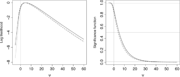
Figure 1: Inferential summaries for the illustrative single-channel data. Left panel: profile relative log likelihood $\ell_{\mathrm{p}}(\psi)-\ell_{\mathrm{p}}(\widehat{\psi})$ (dashes), $-r^{*}(\psi)^{2}/2$ (solid) and $-r_{B}^{*}(\psi)^{2}/2$ (dots). Right panel: $\Phi\{r(\psi)\}$ (dashes), $\Phi\{r^{*}(\psi)\}$ (solid) and $\Phi\{r^{*}_{B}(\psi)\}$ (dots). Horizontal lines are at values $0.99$, $0.01$ and $0.5$, and give respectively the lower and upper bounds of a confidence interval of level 0.98, and a median unbiased estimate of $\psi$. The intersection of a significance function with the vertical line at $\psi=0$ gives the corresponding $p$-value for testing the hypothesis $\psi=0$ against $\psi>0$.

One minus the value of the significance function at $\psi=0$ gives the significance probability for testing the presence of a signal, namely the $p$-value for testing the hypothesis $\psi=0$ against the one-sided hypothesis $\psi>0$. In the present example, $\Phi\{r(0)\}=0.837$ and $\Phi\{r^{*}(0)\}=0.873$, thus giving $p$-values respectively equal to $0.163$ and $0.127$, both weak evidence of a positive signal. This is hardly surprising, as $y_{1}=1$: just one event has been observed.

As explained in Section 2, the significance function provides lower and upper bounds for any desired confidence level. Figure 1 indicates the choice of lower and upper bounds for level $0.99$. In particular, for the modified likelihood root, we get $\Phi\{r^{*}(\psi^{*}_{0.01})\}=0.99$ and $\Phi\{r^{*}(\psi^{*}_{0.99})\}=0.01$, with $\psi^{*}_{0.99}=-2.603$ and $\psi^{*}_{0.01}=36.519$. It is possible for these limits to be negative, as happens in the present case for the lower bound. In such instances, we take as a limit the maximum $\max(\psi^{*}_{\alpha},0)$ of the actual limit, $\psi^{*}_{\alpha}$, and the lower physically admissible value of zero. The fact that the lower bound is zero in this case is coherent with the $p$-value for testing a positive signal. In fact, a right-tail confidence interval of level $0.99$ in this case contains all possible parameter values, also including $0$; thus it is $[0,+\infty)$. A left-tail confidence interval is $[0,36.510)$, although its usual interpretation makes it ill-suited to claim the presence of signal. The analogous limits obtained using the likelihood root $r(\psi)$ are $\psi_{0.99}=-2.644$ and $\psi_{0.01}=33.835$.

In extreme situations confidence limits at any standard choice of $\alpha$ may be negative, thus giving confidence intervals including only the value $\psi=0$. We see this feature of the method as a perfectly sensible frequentist answer (see also Cox (2006), Example 3.7). In such instances the $p$-value for testing $\psi=0$ against the alternative $\psi>0$ would be very close to $1$, thus strongly suggesting that there is no positive signal. However, doubt is cast on the model when no physically realistic parameter value is supported by the observed data.

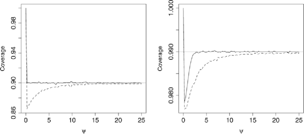
Figure 2: Coverages of $0.90$ (left panel) and $0.99$ (right panel) upper bounds from 39,700 simulated datasets from a single channel, with large uncertainty in the nuisance parameters, from the Banff Challenge. The solid and dashed lines correspond respectively to $r^{*}(\psi)$ and $r_{B}^{*}(\psi)$. The ideal coverage is shown by the horizontal lines.

In the Banff Challenge only coverage of left-tail confidence intervals (upper bounds) was tested, though we regard $p$-values and lower bounds as more appropriate for inference on $\psi$. Figure 2 shows the coverage of $0.90$ and $0.99$ confidence limits as functions of $\psi$ for a set of 39,700 simulated datasets with large variability in the values of the nuisance parameters. The coverage is very good, with only minor undercoverage in the $0.99$ upper bounds when the parameter $\psi$ is small. Similar results were obtained for another set of simulated datasets, with smaller variability in the nuisance parameters. We also performed some simulation studies with a variety of parameter values, and found that our procedure is typically highly accurate. Table 1 displays results in the worst scenario that we found. Apart from some minor issues in the right tail, $r^{*}$ performs extremely well.

In some boundary cases with $y_{1}=0$ it is impossible to compute the quantities needed for (2). In these rare cases we replaced $r^{*}(\psi)$ with $r(\psi)$.

3.3 Several Channels

Our approach extends easily to multiple channels. When there are $n>1$ channels, the nuisance parameters $(\lambda_{1k},\lambda_{2k})$ are channel-specific, so the profile log likelihood is simply the sum of profile log likelihood contributions for the individual channels, which is then maximized numerically to get the overall estimate $\widehat{\theta}=(\widehat{\psi},\widehat{\lambda})$.

The remaining ingredient needed to compute the modified likelihood root $r^{*}(\psi)$ is the $2n+1$-dimensional canonical parameter $\varphi(\theta)$, which can be obtained using (5) and (3). The first element of $\varphi(\theta)$ is

$$\sum_{k=1}^{n}e^{\widehat{\lambda}_{2k}-\widehat{\lambda}_{1k}}\log(\psi e^{\lambda_{2k}-\lambda_{1k}}+e^{\lambda_{2k}}),$$

and the $2n$ other elements are

$$\widehat{\psi}e^{\widehat{\lambda}_{2k}-\widehat{\lambda}_{1k}}\log(\psi e^{\lambda_{2k}-\lambda_{1k}}+e^{\lambda_{2k}})$$

$$\quad{}+u_{j}(\lambda_{2k}-\lambda_{1k})e^{\widehat{\lambda}_{2k}-\widehat{\lambda}_{1k}},$$

$$e^{\widehat{\lambda}_{2k}}\log(\psi e^{\lambda_{2k}-\lambda_{1k}}+e^{\lambda_{2k}})+t_{j}\lambda_{2k}e^{\widehat{\lambda}_{2k}},$$

$$\eqntext{k=1,\ldots,n.}$$ (7)

Any affine transformation of $\varphi(\theta)$ would give the same modified likelihood root.

Table 1: Empirical coverage probabilities in a single-channel simulation with 10,000 replications, $\psi=1$, $\log\beta=1.1$, $\log\gamma=0$, $t=33$ and $u=100$

Probability	$\bolds r$	$\bolds{r^{*}}$	$\bolds{r^{*}_{B}}$
0.0100	0.0080	0.0092	0.0104
0.0250	0.0225	0.0253	0.0263
0.0500	0.0437	0.0500	0.0514
0.1000	0.0887	0.0995	0.1019
0.5000	0.4669	0.5054	0.5045
0.9000	0.8947	0.9051	0.9036
0.9500	0.9186	0.9461	0.9320
0.9750	0.9736	0.9809	0.9785
0.9900	0.9816	0.9816	0.9816

[]Figures in bold differ from the nominal level by more than simulation error.

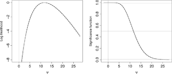
Figure 3: Inferential summaries for the simulated multiple-channel data in Table 2. For details, see caption to Figure 1.

Figure 3 gives the profile and adjusted profile log likelihoods for $\psi$ and the corresponding significance functions for an illustrative dataset with $n=10$ channels shown in Table 2. The interpretation of these plots is the same as for Figure 1. The modified likelihood root gives a $p$-value of $7.709\times 10^{-7}$ for testing the presence of a signal, whereas that based on the likelihood root is $3.124\times 10^{-7}$. The estimates are $\widehat{\psi}^{*}=11.682$ and $\widehat{\psi}=11.487$ and the lower and upper bounds are $\psi^{*}_{0.99}=4.572$, $\psi^{*}_{0.01}=23.191$ and $\psi_{0.99}=4.496$, $\psi^{*}_{0.01}=22.907$. There is strong evidence of a positive signal from these data, though the modified likelihood root $r^{*}(\psi)$ gives weaker support than does the ordinary likelihood root $r(\psi)$. In fact the evidence here corresponds to significance near to the “$5\sigma$” level used by particle physicists when deciding whether or not to announce a discovery (Lyons (2008)).

Table 2: Simulated multiple-channel data

Channel	$\bolds{y_{1}}$	$\bolds{y_{2}}$	$\bolds{y_{3}}$	$\bolds{t}$	$\bolds{u}$
$1$	1	$7$	$5$	15	50
$2$	1	$5$	$12$	17	55
$3$	2	$4$	$2$	19	60
$4$	2	$7$	$9$	21	65
$5$	1	$9$	$6$	23	70
$6$	1	$3$	$5$	25	75
$7$	2	$10$	$10$	27	80
$8$	3	$6$	$12$	29	85
$9$	2	$9$	$7$	31	90
$10$	1	$13$	$13$	33	95

Boundary samples also arise in the multiple-channel case, though less frequently than with a single channel. In such cases we again used the likelihood root $r(\psi)$ for inference on $\psi$.

Figure 4 shows coverages of the $0.90$ and $0.99$ left-tail confidence intervals (upper bounds) computed with the modified likelihood root from 70,000 simulated datasets with $n=10$ from the Banff Challenge. Our approach seems to perform satisfactorily even with as many as 20 nuisance parameters, though there is again some undercoverage for small values of $\psi$. Table 3 reports coverage probabilities for limits at various confidence levels for a simulation performed with $\psi=2$. The results for the modified likelihood root are always within simulation error of the nominal levels, thus giving very accurate inference for $\psi$.

4 Bayesian Inference

4.1 Noninformative Priors

There is a close link between the modified likelihood root and analytical approximations useful for Bayesian inference. Suppose that posterior inference is required for $\psi$ and that the chosen prior density is $\pi(\psi,\lambda)$. Then it turns out that replacing (2) with

$$q_{B}(\psi)=\ell^{\prime}_{\mathrm{p}}(\psi)j_{\mathrm{p}}(\widehat{\psi})^{-1/2}\biggl{\{}{|j_{\lambda\lambda}(\widehat{\theta}_{\psi})|\over|j_{\lambda\lambda}(\widehat{\theta})|}\biggr{\}}^{1/2}{\pi(\widehat{\theta})\over\pi(\widehat{\theta}_{\psi})}$$

in formula (1), where $\ell^{\prime}_{\mathrm{p}}$ is the derivative of $\ell_{\mathrm{p}}(\psi)$ with respect to $\psi$, leads to a Laplace-type approximation to the marginal posterior distribution for $\psi$, that we will denote by $r^{*}_{B}(\psi)$. This may be used to include prior information, but, as mentioned above, the choice of prior density can be vexing. In this section we discuss noninformative Bayesian inference for $\psi$.

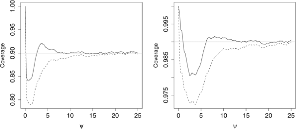
Figure 4: Empirical coverages of $0.90$ (left panel) and $0.99$ (right panel) upper bounds from 70,000 simulated multiple-channel datasets from the Banff Challenge. The solid and dashed lines correspond respectively to $r^{*}(\psi)$ and $r_{B}^{*}(\psi)$.

For models with scalar $\psi$ and a nuisance parameter $\xi$ that is orthogonal to $\psi$ in the sense of Cox and Reid (1987), Tibshirani (1989) shows that up to a certain degree of approximation, a prior density that is noninformative about $\psi$ is proportional to

$$|i_{\psi\psi}(\psi,\xi)|^{1/2}g(\xi)\,d\psi\,d\xi,$$ (8)

where $i_{\psi\psi}(\psi,\xi)$ denotes the $(\psi,\psi)$ element of the Fisher information matrix, and $g(\xi)$ is an arbitrary positive function that satisfies mild regularity conditions. Under further mild conditions (8) is a Jeffreys prior for $\psi$, and it is also a matching prior: following Welch and Peers (1963), Reid, Mukerjee and Fraser (2002) show how (8) yields $(1-\alpha)$ one-sided Bayesian posterior confidence intervals that contain $\psi$ with probability $(1-\alpha)+\mathcal{O}(n^{-1})$ in a frequentist sense. Unfortunately (8) requires one to express the model in terms of an orthogonal parametrization, and this may be impossible. Below we rewrite it in terms of an arbitrary parametrization.

Suppose therefore that the model is parametrized in terms of a scalar interest parameter $\psi$ and a column vector nuisance parameter $\zeta=\zeta(\psi,\xi)$, with the log likelihood written as $\ell^{*}\{\psi,\zeta(\psi,\xi)\}=\ell(\psi,\xi)$. Then the elements of the Fisher information matrices in the two parametrizations are related by the equations

$$i_{\psi\psi} = i^{*}_{\psi\psi}+2\zeta_{\psi}^{\mathrm{T}}i^{*}_{\zeta\psi}+\zeta_{\psi}^{\mathrm{T}}i^{*}_{\zeta\zeta}\zeta_{\psi},$$

$$i_{\xi\psi} = \zeta_{\xi}^{\mathrm{T}}i^{*}_{\zeta\psi}+\zeta_{\xi}^{\mathrm{T}}i^{*}_{\zeta\zeta}\zeta_{\psi},$$ (9)

$$i_{\xi\xi} = \zeta_{\xi}^{\mathrm{T}}i^{*}_{\zeta\zeta}\zeta_{\xi},$$

where $i_{\xi\psi}=\mathrm{E}(-\partial^{2}\ell/\partial\xi\partial\psi^{\mathrm{T}})$, $i^{*}_{\zeta\zeta}=\mathrm{E}(-\partial^{2}\ell^{*}/\break\partial\zeta\partial\zeta^{\mathrm{T}})$, $\zeta_{\psi}=\partial\zeta/\partial\psi$, and so forth, with

Table 3: Empirical coverage probabilities in a multiple-channel simulation with 10,000 replications, $\psi=2$, $\beta=(0.20,0.30,0.40,\ldots,1.10)$, $\gamma=(0.20,0.25,0.30,\ldots,0.65)$, $t=(15,17,19,\ldots,33)$ and $u=(50,55,60,\ldots,95)$

Probability	$\bolds{r}$	$\bolds{r^{*}}$	$\bolds{r^{*}_{B}}$
0.0100	0.0099	0.0101	0.0109
0.0250	0.0244	0.0255	0.0273
0.0500	0.0493	0.0519	0.0542
0.1000	0.0967	0.1012	0.1035
0.5000	0.4869	0.5043	0.5027
0.9000	0.8900	0.9013	0.8942
0.9500	0.9421	0.9499	0.9427
0.9750	0.9687	0.9759	0.9689
0.9900	0.9875	0.9913	0.9864

[]Figures in bold differ from the nominal level by more than simulation error.

$\mathrm{E}$ again denoting expectation. Parameter orthogonality implies that $i_{\xi\psi}\equiv 0$, so provided $\zeta_{\xi}$ is not identically zero, $\xi=\xi(\psi,\zeta)$ is determined by the partial differential equation

$$\zeta_{\psi}=-i^{*-1}_{\zeta\zeta}i^{*}_{\zeta\psi},$$ (10)

which always has a set of solutions for scalar $\psi$. On substituting (10) into the first expression in (4.1), we find that in terms of the original parametrization the required element of the Fisher information matrix may be written as

$$i_{\psi\psi}=i^{*}_{\psi\psi}-i^{*}_{\psi\zeta}i^{*-1}_{\zeta\zeta}i^{*}_{\zeta\psi},$$

whence the noninformative prior (8) may be written as

$$|i^{*}_{\psi\psi}-i^{*}_{\psi\zeta}i^{*-1}_{\zeta\zeta}i^{*}_{\zeta\psi}|^{1/2}$$

(11)

$$\quad{}\cdot g\{\xi(\psi,\zeta)\}|\partial\xi/\partial\zeta|d\psi d\zeta,$$

which requires that the orthogonal parameter $\xi$ be expressed in terms of the original parameters; cf. expression (5) of Tibshirani (1989). In the next section we derive (4.1) for the single- and multiple-channel models of Section 3.

4.2 Application to Poisson Model

The single-channel model may be reparametrized in terms of $\psi$, $\gamma$ and $\zeta=\beta/\gamma$, in which case $Y_{1},Y_{2},Y_{3}$ are independent Poisson variables with means $\gamma(\psi+\zeta),\zeta\gamma t,\gamma u$. This implies that the trinomial density of $(Y_{1},Y_{2},Y_{3})$ conditional on the total $S=Y_{1}+Y_{2}+Y_{3}$ does not depend on $\gamma$, and there is no loss of information on $\psi$ and $\zeta$ if we base inference on the trinomial or more generally the multinomial model (Barndorff-Nielsen (1978), Chapter 10). In particular, frequentist inferences on $\psi$ based on the original model or on the conditional trinomial model lead to exactly the same results. Here $\zeta$ is scalar. Apart from additive constants, the corresponding log likelihood is

$$\ell^{*}(\psi,\zeta) = y_{1}\log(\psi+\zeta)+y_{2}\log\zeta$$

$${}-s\log(\psi+\zeta+u+\zeta t),\quad\psi+\zeta,\zeta>0,$$

and $\mathrm{E}(Y_{1}\mid S=s)=s(\psi+\zeta)/\pi$, $\mathrm{E}(Y_{2}\mid S=s)=st\zeta/\pi$, where $\pi=\psi+\zeta+u+\zeta t$. Thus in this parametrization the Fisher information matrix for the trinomial model has form

$$i^{*}(\psi,\zeta)$$

$$\quad={s\over\pi^{2}(\zeta+\psi)}$$

$$\qquad{}\cdot\pmatrix{u+\zeta t&u-\psi t\cr u-\psi t&\{\psi t(\psi+u)+\zeta u(1+t)\}/\zeta},$$

and the orthogonal parameter is a solution of the equation

$$\zeta_{\psi}=\zeta(\psi t-u)/\{\psi t(\psi+u)+\zeta u(1+t)\},$$

such as

$$\xi(\psi,\zeta) = t\log\zeta+\log(\zeta+\psi)$$

$${}-(1+t)\log(\psi+\zeta+u+\zeta t).$$

It is impossible to express $\zeta$ explicitly as a function of $\psi$ and $\xi$, and hence to use the noninformative prior in the form (8), but (4.1) is readily obtained, and after a little algebra turns out to be proportional to

$$\biggl{[}{\psi t(\psi+u)+\zeta u(1+t)\over\zeta^{2}(\zeta+\psi)^{2}(\psi+\zeta+u+\zeta t)^{3}}\biggr{]}^{1/2}$$ (13)

$$\quad{}\cdot g\biggl{\{}{(\zeta+\psi)\zeta^{t}\over(\psi+\zeta+u+\zeta t)^{1+t}}\biggr{\}}\,d\psi\,d\zeta,$$

$$\eqntext{\zeta,\psi+\zeta>0,}$$

for an arbitrary but smooth and positive function $g$.

If data $(y_{1k},y_{2k},y_{3k},t_{k},u_{k})$ are available for $n$ independent channels, then the conditioning argument above yields $n$ independent trinomial distributions for $(y_{1k},y_{2k},y_{3k})$ conditional on the $s_{k}=y_{1k}+y_{2k}+y_{3k}$, whose probabilities depend on the parameters $\psi,\zeta_{k}$. Apart from an additive constant the log likelihood is

$$\ell^{*}(\psi,\zeta_{1},\ldots,\zeta_{n})$$

$$\quad=\sum_{k=1}^{n}\{y_{1k}\log(\psi+\zeta_{k})$$

$$\hskip 38.5pt{}+y_{2k}\log\zeta_{k}-s_{k}\log(\psi+\zeta_{k}+u_{k}+\zeta_{k}t_{k})\},$$

where $\psi>-\min(\zeta_{1},\ldots,\zeta_{n})$ and $\zeta_{1},\ldots,\zeta_{n}>0$. Calculations like those leading to (13) reveal that the noninformative prior for $\psi$ is proportional to

$$\Biggl{|}\sum_{k=1}^{n}{s_{k}t_{k}u_{k}}/(\zeta_{k}+\psi+u_{k}+\zeta t_{k})$$

$$\quad\hskip 5.6pt{}\cdot\{\psi(\psi+u_{k})t_{k}+\zeta_{k}u_{k}(1+t_{k})\}\Biggr{|}^{1/2}$$ (14)

$$\quad{}\cdot\prod_{k=1}^{n}{\psi(\psi+u_{k})t_{k}+\zeta_{k}u_{k}(1+t_{k})\over\zeta_{k}(\zeta_{k}+\psi)(\zeta_{k}+\psi+u_{k}+\zeta_{k}t_{k})},$$

times an arbitrary function of the quantities

$$\xi_{k}(\psi,\zeta_{k}) = t_{k}\log\zeta_{k}+\log(\zeta_{k}+\psi)$$ (15)

$${}-(1+t_{k})\log(\psi+\zeta_{k}+u_{k}+\zeta_{k}t_{k}),$$

$$\eqntext{k=1,\ldots,n.}$$

Although (4.2) depends on the data through $s_{1},\ldots,s_{n}$, these are constants under the trinomial model, as are the $t_{k}$ and $u_{k}$ under both Poisson and trinomial models. The presence of $s_{k}t_{k}u_{k}$ in the first term of (4.2) has the heuristic explanation that a channel for which this product is large will contain more information about its nuisance parameters.

4.3 Numerical Results

We first consider the single-channel data analyzed in Section 3.2, with $y_{1}=1$, $y_{2}=8$, $y_{3}=14$, and $t=27$, $u=80$. The dotted lines in Figure 1 show the approximate posterior function, $-r^{*}_{B}(\psi)^{2}/2$, and the corresponding significance function obtained using the noninformative prior (13), with $g$ taken to be a constant function.

Typically the prior density yields larger lowerbounds and smaller upper bounds than those obtained from the frequentist solution, because the effect of the prior is to inject information about the parameter of interest. In the present case, the estimate $\widehat{\psi}_{B}^{*}=4.9182$, which satisfies $\Phi\{r^{*}_{B}(\widehat{\psi}_{B}^{*})\}=0.5$, is smaller than the corresponding estimate obtained using $r^{*}(\psi)$, and the $0.99$ lower and upper bounds are respectively given by $\Phi\{r^{*}_{B}(\psi^{*}_{B;0.01})\}=0.99$ and $\Phi\{r^{*}_{B}(\psi^{*}_{B;0.99})\}=0.01$, with $\psi^{*}_{B;0.99}=-1.820$ and $\psi^{*}_{B;0.01}=35.094$.

The $p$-value for testing the hypothesis $\psi=0$against the one-sided hypothesis $\psi>0$ is equal to $1-\Phi\{r^{*}_{B}(0)\}=0.1063$, which is again a weak evidence of a positive signal.

The coverage properties of the noninformativeBayesian solution are similar to but not quite so good as those of the frequentist solution, as shown in Figure 2 and by the simulation results reported in the last column of Table 1.

Similar behavior is seen in the multichannel case. Figure 3 shows the approximate posterior function, $-r^{*}_{B}(\psi)^{2}/2$, and the corresponding significance function obtained using the noninformative prior (4.2) times a constant function of $\xi_{k}(\psi,\zeta_{k})$, $k=1,\ldots,n$, for the data in Table 2. The approximate Bayesian solution gives a $p$-value of $4.865\times 10^{-8}$ for testing the presence of a signal, smaller than that obtained from the frequentist solutions in Section 3.3. The estimate is $\widehat{\psi}_{B}^{*}=11.632$ and the lower and upper bounds are $\psi^{*}_{B;0.99}=4.699$ and $\psi^{*}_{B;0.01}=23.030$. There is stronger evidence of a positive signal from this approach than from the modified likelihood root $r^{*}(\psi)$ and the ordinary likelihood root $r(\psi)$. However, simulation results reported in Figure 4 and Table 3 show that the coverage of confidence sets based on the approximate Bayesian solution is not quite so good as for sets based on the modified likelihood root.

5 Discussion

In this paper we propose procedures based on modern likelihood theory for detecting a signal in the presence of background noise, using a simple statistical model. We suggest the use of the significance function based on the modified likelihood root as a comprehensive summary of the information for the parameter given the model and the observed data, from which $p$-values and one- or two-sided confidence limits can be obtained directly.

Even when there are 20 nuisance parameters, our frequentist procedure appears to give essentially exact inferences for the signal parameter $\psi$. Its noninformative Bayesian counterpart performs slightly worse in terms of coverage of confidence intervals and levels for tests, but provides slightly better point estimates as solutions to the equation $\Phi\{r^{*}_{B}(\psi)\}=0.5$, analogous to median unbiased estimates. The most serious departures from the correct coverage are for small values of $\psi$, corresponding to weak signals, and arise because in such cases very low counts $y_{1}$ corresponding to the observed signal are quite likely to arise. The case of a weak signal seems to be of little practical interest, because in such cases no strong significance can be obtained. Although the Banff Challenge concerned significance at the 90% and 99% levels, both general theory and the accuracy of our results suggest that similar precision can be expected for much more extreme significance levels.

If $y_{1}=0$ our higher-order approaches break down, though a closely related first-order inference is available. Such cases are scientifically uninteresting, but to avoid difficulties it is tempting to replace $y_{1}$ by $y_{1}+c$, where $c$ is a small positive quantity. Firth (1993) investigates under what circumstances this modification yields an improved estimate of the interest parameter in exponential family models, taken on the canonical scale of the exponential family. Our model is not a linear exponential family, but ideas of Kosmidis (2007) might be used to choose $c$ to yield an improved estimate of $\psi$. Our main interest is in confidence intervals and tests, however, and since Firth’s correction corresponds to use of a default Jeffreys prior and we have found that use of a noninformative prior does not improve coverage properties of our method, one should not be optimistic about the effect of this correction in our context.

In some instances the method may lead to empty confidence intervals or intervals including only the value $\psi=0$. Though galling to the experimenters, this is not a critical problem from a frequentist perspective. On the one hand, even in such extreme samples the confidence function would yield a $p$-value to test for the presence of a signal, and on the other hand, the concentration of the likelihood and significance functions in a region of physically meaningless values of the parameter might suggest that the model is inappropriate.

References

- Barndorff-Nielsen (1978) Barndorff-Nielsen, O. E. (1978). Information and Exponential Families in Statistical Theory. Wiley, New York. \MR0489333
- Barndorff-Nielsen and Cox (1994) Barndorff-Nielsen, O. E. and Cox, D. R. (1994). Inference and Asymptotics. Chapman and Hall, London. \MR1317097
- Brazzale, Davison and Reid (2007) Brazzale, A. R., Davison, A. C. and Reid, N. (2007). Applied Asymptotics: Case Studies in Small Sample Statistics. Cambridge Univ. Press, Cambridge. \MR2342742
- Cox (2006) Cox, D. R. (2006). Principles of Statistical Inference. Cambridge Univ. Press, Cambridge. \MR2278763
- Cox and Reid (1987) Cox, D. R. and Reid, N. (1987). Parameter orthogonality and approximate conditional inference (with discussion). J. Roy. Statist. Soc. Ser. B 49 1–39. \MR0893334
- Davison (2003) Davison, A. C. (2003). Statistical Models. Cambridge Univ. Press, Cambridge. \MR1998913
- Davison, Fraser and Reid (2006) Davison, A. C., Fraser, D. A. S. and Reid, N. (2006). Improved likelihood inference for discrete data. J. Roy. Statist. Soc. Ser. B 68 495–508. \MR2278337
- Firth (1993) Firth, D. (1993). Bias reduction of maximum likelihood estimates. Biometrika 80 27–38. \MR1225212
- Fraser, Reid and Wong (2004) Fraser, D. A. S., Reid, N. and Wong, A. C. M. (2004). Inference for bounded parameters. Phys. Rev. D 69 033002.
- O’Hagan and Forster (2004) O’Hagan, A. and Forster, J. J. (2004). Kendall’s Advanced Theory of Statistics. Volume 2B: Bayesian Inference, 2nd ed. Hodder Arnold, London.
- Jeffreys (1961) Jeffreys, H. (1961). Theory of Probability, 3rd ed. Clarendon Press, Oxford. \MR0187257
- Kosmidis (2007) Kosmidis, I. (2007). Bias reduction in exponential family nonlinear models. Ph.D. thesis, Dept. Statistics, Univ. Warwick.
- Lyons (2008) Lyons, L. (2008). Open statistical issues in particle physics. Ann. Appl. Statist. 2 887–915.
- Mandelkern (2002) Mandelkern, M. (2002). Setting confidence intervals for bounded parameters (with discussion). Statist. Sci. 17 149–172. \MR1939335
- Pace and Salvan (1997) Pace, L. and Salvan, A. (1997). Principles of Statistical Inference from a Neo-Fisherian Perspective. World Scientific, Singapore. \MR1476674
- Reid (2003) Reid, N. (2003). Asymptotics and the theory of inference. Ann. Statist. 31 1695–1731. \MR2036388
- Reid, Mukerjee and Fraser (2002) Reid, N., Mukerjee, R. and Fraser, D. A. S. (2002). Some aspects of matching priors. In Mathematical Statistics and Applications: Festschrift for Constance van Eeden (M. Moore, S. Froda and C. Léger, eds.). Lecture Notes—Monograph Series 42 31–44. IMS, Hayward, CA. \MR2138284
- Severini (2000) Severini, T. A. (2000). Likelihood Methods in Statistics. Clarendon Press, Oxford. \MR1854870
- Tibshirani (1989) Tibshirani, R. J. (1989). Noninformative priors for one parameter of many. Biometrika 76 604–608. \MR1040654
- Welch and Peers (1963) Welch, B. L. and Peers, H. W. (1963). On formulae for confidence points based on integrals of weighted likelihoods. J. Roy. Statist. Soc. Ser. B 25 318–329. \MR0173309