Large Deviations Analysis for Distributed Algorithms in an Ergodic Markovian Environment

Abstract

We provide a large deviations analysis of deadlock phenomena occurring in distributed systems sharing common resources. In our model transition probabilities of resource allocation and deallocation are time and space dependent. The process is driven by an ergodic Markov chain and is reflected on the boundary of the $d$-dimensional cube. In the large resource limit, we prove Freidlin-Wentzell estimates, we study the asymptotic of the deadlock time and we show that the quasi-potential is a viscosity solution of a Hamilton-Jacobi equation with a Neumann boundary condition. We give a complete analysis of the colliding 2-stacks problem and show an example where the system has a stable attractor which is a limit cycle.

Short Title: Distributed Algorithms in an Ergodic Environment

Key words and phrases: Large deviations, distributed algorithm, averaging principle, Hamilton-Jacobi equation, viscosity solution

AMS subject classifications: Primary 60K37; secondary 60F10, 60J10

1 Introduction

Distributed algorithms are related to resource sharing problems. Colliding stacks problems and the banker algorithm are among the examples which have attracted large interest over the last decades in the context of deadlock prevention on multiprocessor systems. Knuth [22], Yao [32], Flajolet [15], Louchard, Schott et al. [26, 27, 28] have provided combinatorial or probabilistic analysis of these algorithms in the $2$-dimensional case under the assumption that transition probabilities (of allocation or deallocation) are constant. Maier [29] proposed a large deviations analysis of colliding stacks for the more difficult case where the transition probabilities are non-trivially state-dependent. More recently Guillotin-Plantard and Schott [17, 18] analyzed a model of exhaustion of shared resources where allocation and deallocation requests are modeled by time-dependent dynamic random walks. In [8], the present authors provided a probabilistic analysis of the $d$-dimensional banker algorithm when transition probabilities evolve, as time goes by, along the trajectory of an ergodic Markovian environment, whereas the spatial parameter just acts on long runs. The analysis in [8] relies on techniques from stochastic homogenization theory. In this paper, we consider a similar dynamics, but in a stable regime instead of a neutral regime as in our previous paper, and we provide an original large deviations analysis in the framework of Freidlin-Wentzell theory. Given the environment, the process of interest is a Markov process depending on the number $m$ of available resource, with smaller and more frequent jumps as $m\to\infty$, see (3.1). A number of monographs and papers have been written on this theory: [14], [16] and [19] for random environment, [10], [12], [21] and [20] for reflected processes, [3], [9] and [30] for homogeneous Markov processes. However, our framework, including both reflections on the boundary and averaging on the Markovian environment, is not covered by the current literature, and we establish here the large deviations principle. We prove that the time of resource exhaustion then grows exponentially with the size of the system – instead of polynomially in the neutral regime of [8]– and has exponential law as limit distribution. Then, we study the quasi-potential, which solves, according to general wisdom, some Hamilton-Jacobi equation: in view of the reflection on the hypercube, which boundary is non-regular, we prove this fact in the framework of viscosity solution, and study the optimal paths (so-called instantons).

We investigate in details a particular situation introduced in a beautiful paper of Maier [29], where the motion in each direction depends on the corresponding coordinate only, with the additional dependence in the Markovian environment. In fact, we discover the quasi-potential by observing that the discrete process has an invariant measure, for which we study the large deviations properties. We can then use the characterization in terms of Hamilton-Jacobi equation to bypass the Hamiltonian mechanics approach of [29]. For the deadlock phenomenon, we finally obtain a (even more) complete picture (after an even shorter work). To the best of our knowledge, this is first such analysis developed for space-time inhomogeneous distributed algorithms.

The organization of this paper is as follows: we discuss our probabilistic model in Section 2. In Section 3 we prove a Large Deviations Principle. Deadlock phenomenon analysis is done rigorously with much details in Section 4. In Section 5 we illustrate with the two-stacks model. In Section 6 we work out an example where the system has (in the large scale resource limit $m\rightarrow\infty$) a stable attractor which is a limit cycle. Some technical proofs of results stated in Section 4 are deferred to Appendix (Section 7).

2 The Model

The environment is given by a Markov chain $(\xi_{n})_{n\geq 0}$ defined on $(\Omega,{\cal A},{\mathbb{P}})$ with values in a finite space $E$, $N=|E|$. We denote by $P$ its transition matrix, $P(k,\ell)={\mathbb{P}}(\xi_{n+1}=\ell|\xi_{n}=k)$ for $k,\ell\in E$.

The steps of the walker take place in the set

$${\mathcal{V}}=\{e_{1},-e_{1},\dots,e_{d},-e_{d}\}\;,$$

where $(e_{i})_{1\leq i\leq d}$ denotes the canonical basis of ${\mathbb{Z}}^{d}$, and are reflected along the boundary of the hypercube $[0,m]^{d}$, for a large integer $m$.

Following [8], we first discuss the dynamics of the walk in the non-reflected setting. The displacement of the walker has then law $(p(s/m,i,v);v\in{\mathcal{V}})$, when located at $s$ and when the environment is $i$. To obtain a stochastic representation – which is, in contrast to [8], needed here – , we are also given, on $(\Omega,{\mathcal{A}},\mathbb{P})$, a sequence $(U_{n})_{n\geq 0}$ of independent and uniformly distributed random variables on $(0,1)$, independent of the family $(\xi_{n})_{n\geq 0}$. Denoting by $f:(s,i,v)\in\mathbb{R}^{d}\times E\times(0,1)\rightarrow{\mathcal{V}}$ the inverse of the cumulative distribution function of $(p(s,i,u))_{u\in{\mathcal{V}}}$ (for an arbitrary order on ${\mathcal{V}}$), we have

$${\mathbb{P}}\{f(s,i,U_{n})=v\}=p(s,i,v)\;,$$

so that the position of the walker can be defined recursively by

$$S_{n+1}=S_{n}+f(S_{n}/m,\xi_{n},U_{n}).$$ (2.1)

The reflected walk is obtained by symmetry with respect to the faces of the hypercube. Denoting by ${\rm Id}$ the identity mapping on $\mathbb{R}^{d}$ and by $\Pi$ (resp. $\Pi^{(m)}$) the projection on the hypercube $[0,1]^{d}$ (resp. $[0,m]^{d}$), we define recursively the position of the walker by

$$\begin{split}X_{n+1}&=(2\Pi^{(m)}-{\rm Id})\bigl{(}X_{n}+f(X_{n}/m,\xi_{n},U_{n})\bigr{)}\\ &=m(2\Pi-{\rm Id})\bigl{(}X_{n}/m+(1/m)f(X_{n}/m,\xi_{n},U_{n})\bigr{)}.\end{split}$$ (2.2)

When $X_{n}$ is on the boundary and $X_{n}+f(X_{n}/m,\xi_{n},U_{n})$ is outside the hypercube, $X_{n+1}$ is the symmetric point of $X_{n}+f(X_{n},\xi_{n},U_{n})$ with respect to the face containing $X_{n}$ and orthogonal to $f(X_{n}/m,\xi_{n},U_{n})$, i.e. $X_{n+1}=X_{n}-f(X_{n}/m,\xi_{n},U_{n})$. The kernel $q$ of the walk $(X_{n})_{n\geq 1}$ has the following form. When located at $x\in(0,m)^{d}\cap\mathbb{Z}^{d}$ and when the environment is $i$, the jump of the walker has law $(q(x/m,i,v)=p(x/m,i,v);v\in{\mathcal{V}})$. On the boundary, the reflection rules may be expressed as follows: if $x_{\ell}/m=1$ ($x_{\ell}$ is the $\ell$th coordinate of $x$), $q(x/m,i,e_{\ell})=0$ and $q(x/m,i,-e_{\ell})=p(x/m,i,e_{\ell})+p(x/m,i,-e_{\ell})$ ; if $x_{\ell}=0$, $q(x/m,i,-e_{\ell})=0$ and $q(x/m,i,-e_{\ell})=p(x/m,i,e_{\ell})+p(x/m,i,-e_{\ell})$.

We could choose another reflection rule by setting $X_{n+1}=\Pi^{(m)}(X_{n}+f(X_{n}/m,\xi_{n},U_{n}))$. Such a choice wouldn’t change anything to the proofs given in the paper, except the proof of Theorem 4.9 which uses the fact that the steps of $(X_{n})_{n\geq 0}$ are always non-zero.

Following (2.1), we can write

$$X_{n+1}=X_{n}+g(X_{n}/m,\xi_{n},U_{n})\;,$$ (2.3)

where $g:(x,i,v)\in\mathbb{R}^{d}\times E\times(0,1)\rightarrow{\mathcal{V}}$ is the inverse of the cumulative distribution function of $(q(x,i,u))_{u\in{\mathcal{V}}}$. Of course, $g(x,i,v)=f(x,i,v)$ for $x\in(0,1)^{d}$. On the boundary, $x_{\ell}=1\Rightarrow g_{\ell}(x,i,v)\leq 0$ and $x_{\ell}=0\Rightarrow g_{\ell}(x,i,v)\geq 0$.

The process $(\xi_{n},X_{n})_{n\geq 0}$ is a Markov chain with transition probabilities

$$\ {\mathbb{P}}\bigl{\{}\xi_{n+1}=k,X_{n+1}=v+X_{n}|{\mathcal{F}}^{\xi,X}_{n}\bigr{\}}=P(\xi_{n},k)q(X_{n}/m,\xi_{n},v),$$

where ${\mathcal{F}}^{\xi,X}_{n}=\sigma\{\xi_{0},\dots,\xi_{n},X_{0},\dots,X_{n}\}$. In particular, for $x\in{\mathbb{Z}}^{d}$ and for a probability measure $\nu$ on $E$, we can write ${\mathbb{P}}^{\nu}_{x/m}$ to indicate that the chain starts under the measure $\delta_{x}\otimes\nu$. In many cases, we just write ${\mathbb{P}}_{x/m}$ (resp. ${\mathbb{P}}^{\nu}$): this means that the law of the environment (resp. of the walker) is arbitrary. And, of course, the notation $\mathbb{P}$ means that both the initial conditions of the walker and of the environment are arbitrary.

2.1 Main Assumptions

In the whole paper, $\langle\cdot,\cdot\rangle$ and $|\cdot|$ stand for the Euclidean scalar product and the Euclidean norm in $\mathbb{R}^{d}$. The symbols $|\cdot|_{1}$ and $|\cdot|_{\infty}$ denote the standard $\ell^{1}$ and $\ell^{\infty}$ norms in $\mathbb{R}^{d}$.

From a purely practical point of view, the values of $p(x,i,v)$ for $x$ outside the hypercube $[0,1]^{d}$ are totally useless. In the sequel, we refer, for pedagogical reasons, to the non-reflected walk: in such cases, we need $p(x,i,v)$ to be defined for all $x\in\mathbb{R}^{d}$. This is the reason why the variable $x$ lies in $\mathbb{R}^{d}$ in the following assumptions.

In formulas (2.1) and (2.2), the division by $m$ indicates that the dependence of the transition kernel on the position of the walker takes place at scale $m$. For large $m$, the space dependence is mild, since we will assume all through the paper the following smoothness property:
Assumption (A.1). There exists a finite constant $K$ such that $|p(x,i,v)-p(y,i,v)|\leq K|x-y|,\ x,y\in{\mathbb{R}}^{d},i\in E,v\in{\mathcal{V}}$.

For technical reasons, which are explained in the paper, we impose the following ellipticity condition:

Assumption (A.2). For all $x\in\mathbb{R}^{d}$, $i\in E$ and $v\in{\mathcal{V}}$, $p(x,i,v)>0$. By continuity, $\inf\{p(x,i,v);\,x\in[0,1]^{d},\,i\in E,\,v\in{\mathcal{V}}\}>0$.

We also assume the environment to be ergodic and to obey the large deviations principle for Markov chains. We thus impose the following sufficient conditions:
Assumption (A.3). The matrix $P$ is irreducible on $E$. Its unique invariant probability measure is denoted by $\mu$.
In particular, the following vector-valued function is smooth:

$$\bar{f}(x)={\mathbb{E}}^{\mu}f(x,\xi,U)=\sum_{v\in{\mathcal{V}}}v\;{\mathbb{E}}^{\mu}p(x,\xi,v)\;,\quad x\in{\mathbb{R}}^{d}\;;$$ (2.4)

the above expectations are taken over independent variables $\xi,U$, where $\xi$ has the distribution $\mu$ and $U$ is uniformly distributed on [0,1].

For the deadlock time analysis, another assumption will be necessary (see (A.4) in Section 4).

2.2 Continuous Counterpart and Skorohod Problem

Because of the reflection phenomenon, we briefly recall what the Skorohod problem is (we refer to [23] for a complete overview of the subject). For each continuous mapping $w:t\in[0,+\infty)\mapsto w_{t}\in\mathbb{R}^{d}$, with $w_{0}\in[0,1]^{d}$, there exists a unique continuous mapping $t\in[0,+\infty)\mapsto(x_{t},k_{t})\in[0,1]^{d}\times\mathbb{R}^{d}$, with $k$ of bounded variation on any bounded sets, such that:

$$\forall t\geq 0\;,\quad w_{t}=x_{t}+k_{t}\;,\quad k_{t}=\int_{0}^{t}n_{s}d|k|_{s}\;,\quad|k|_{t}=\int_{0}^{t}{\mathbf{1}}_{\{x_{s}\in\partial[0,1]^{d}\}}d|k|_{s}\;,$$ (2.5)

where $n_{s}\in{\mathcal{N}}(x_{s})$, ${\mathcal{N}}(x)$ denoting for $x\in\partial[0,1]^{d}$ the set of unit outward normals to $\partial[0,1]^{d}$ at $x$, that is

$${\mathcal{N}}(x)=\{v\in\mathbb{R}^{d}:\,|v|=1,\,v_{\ell}=0{\rm\ if\ }x_{\ell}\in(0,1),\,v_{\ell}\leq 0{\rm\ if\ }x_{\ell}=0,\,v_{\ell}\geq 0{\rm\ if\ }x_{\ell}=1\}.$$

When $x$ is in the relative interior of a face of the hypercube, ${\mathcal{N}}(x)$ is obviously empty.

It can be proved (see again [23]) that, for every $T>0$, the mapping $\Psi:(w_{t})_{0\leq t\leq T}\mapsto(x_{t})_{0\leq t\leq T}$ is continuous from ${\mathcal{C}}_{[0,1]^{d}}([0,T];\mathbb{R}^{d})$ into itself with respect to the supremum norm (it is even $1/2$-Hölder continuous on compact subsets of ${\mathcal{C}}_{[0,1]^{d}}([0,T];\mathbb{R}^{d})$); here and below, ${\mathcal{C}}_{A}([0,T];\mathbb{R}^{d})$ denotes the set of continuous functions from $[0,T]$ to $\mathbb{R}^{d}$ with an initial datum in $A$. Moreover, if $w$ is absolutely continuous, then $x$ and $k$ are also absolutely continuous (see [23, Theorem 2.2]).

Equation (2.2) corresponds to a Euler scheme for a Reflected Differential Equation (RDE in short). An RDE is an ordinary differential equation, but driven by a pushing process $k$ as in (2.5). For a given initial condition $x_{0}\in[0,1]^{d}$ and a given jointly measurable and $x$-Lipschitz continuous mapping $b:\mathbb{R}_{+}\times[0,1]^{d}\rightarrow\mathbb{R}^{d}$, the RDE

$$\forall T>0,\ (x_{t})_{0\leq t\leq T}=\Psi\biggl{[}\biggl{(}x_{0}+\int_{0}^{t}b(s,x_{s})ds\biggr{)}_{0\leq t\leq T}\biggr{]}\;,$$ (2.6)

admits a unique solution (see again [23]). This solution satisfies the equation

$$\forall t\geq 0,\ x_{t}=x_{0}+\int_{0}^{t}b(s,x_{s})ds-k_{t}\;,$$

with $k$ as in (2.5). In this case, $x$ and $k$ are absolutely continuous.

Reflected equations driven by Lipschitz continuous coefficients are stable. By [23, Lemma 3.1], we can prove that for every $T>0$, there exists a constant $C_{T}\geq 0$, such that, for any $x_{0},y_{0}\in[0,1]^{d}$, the solutions $(x_{t})_{0\leq t\leq T}$ and $(y_{t})_{0\leq t\leq T}$ to (2.6) with $x_{0}$ and $y_{0}$ as initial conditions satisfy $\sup_{0\leq t\leq T}|x_{t}-y_{t}|\leq C_{T}|x_{0}-y_{0}|$.

When $b(s,x)=\bar{f}(x)$, we denote by $(\chi_{t}^{x_{0}})_{t\geq 0}$ the unique solution to the averaged reflected differential equation

$$\forall t\geq 0,\ x_{t}=x_{0}+\int_{0}^{t}\bar{f}(x_{s})ds-k_{t}.$$ (2.7)

3 Large Deviations Principle

We now denote the process $X$ by $X^{(m)}$ to indicate the dependence on the parameter $m$. In what follows, we investigate an interpolated version of the rescaled process $(m^{-1}X_{\lfloor mt\rfloor}^{(m)})_{t\geq 0}$, namely

$$\bar{X}^{(m)}_{t} = (2\Pi-{\rm Id})\bigl{(}m^{-1}X_{\lfloor mt\rfloor}^{(m)}+(t-m^{-1}\lfloor mt\rfloor)f(m^{-1}X_{\lfloor mt\rfloor}^{(m)},\xi_{\lfloor mt\rfloor},U_{\lfloor mt\rfloor})\bigr{)}\;,\quad t\geq 0$$ (3.1)

$$= m^{-1}X_{\lfloor mt\rfloor}^{(m)}+(t-m^{-1}\lfloor mt\rfloor)g(m^{-1}X_{\lfloor mt\rfloor}^{(m)},\xi_{\lfloor mt\rfloor},U_{\lfloor mt\rfloor})\;,\quad t\geq 0$$

We note that the hyperbolic scaling is different from the diffusive scaling in [8]. The process $(\bar{X}^{(m)}_{t})_{t\geq 0}$ is continuous and $\bar{X}^{(m)}_{k/m}=X_{k}^{(m)}$ for any integer $k\in{\mathbb{N}}$.

3.1 Heuristics for the Non-reflected Walk

We first look, for pedagogical reasons, at the non-reflected case. We thus consider

$$\bar{S}^{(m)}_{t}=m^{-1}S_{\lfloor mt\rfloor}^{(m)}+(t-m^{-1}\lfloor mt\rfloor)f(m^{-1}S_{\lfloor mt\rfloor},\xi_{\lfloor mt\rfloor},U_{\lfloor mt\rfloor})\;,\quad{t\geq 0}\;.$$

(As for $X$, we indicate the dependence on $m$ in $S$.) In light of Assumptions (A.1–3), we expect the global effect of the environment process $(\xi_{n})_{n\geq 0}$ to reduce for large time to a deterministic one. More precisely, if the initial position is such that $\bar{S}^{(m)}_{0}\to x$ as $m\to\infty$, we expect $(\bar{S}^{(m)})_{m\geq 1}$ to converge in probability, uniformly on compact sets, to the solution $x_{\cdot}$ of the (averaged) ordinary differential equation

$$\dot{x}_{t}=\bar{f}(x_{t})\;,\quad x_{0}=x\;,$$ (3.2)

that is $\lim_{m\to\infty}\rho_{0,T}(\bar{S}^{(m)}_{\cdot},x_{\cdot})=0$ for all $T>0$, where $\rho_{0,T}(\phi,\psi)=\sup\{|\phi_{t}-\psi_{t}|;\,t\in[0,T]\}$ denotes the distance in supremum norm on the space ${\mathcal{C}}([0,T];\mathbb{R}^{d})$ of continuous functions from $[0,T]$ into $\mathbb{R}^{d}$.

Loosely speaking, the Large Deviations Principle (LDP in short) for $(\bar{S}^{(m)}_{\cdot})_{m\geq 1}$ follows from the Freidlin and Wentzell theory [16, Chapter 7], or at least from a variant of it as explained below. The idea is the following. The irreducible Markov chain $(\xi_{n})_{n\geq 0}$ with a finite state space obeys a LDP (see [9, Theorem 3.1.2, Exercise 3.1.4]). In particular, the function $H$ defined for $x,\alpha\in\mathbb{R}^{d}$ by

$$H(x,\alpha) = \lim_{n\to\infty}\frac{1}{n}\ln{\mathbb{E}}^{i}\exp\big{\langle}\alpha,\sum_{k=1}^{n}f(x,\xi_{k},U_{k})\rangle$$

$$= \lim_{n\to\infty}\frac{1}{n}\ln{\mathbb{E}}^{i}\prod_{k=1}^{n}\left[\sum_{v\in{\mathcal{V}}}e^{\langle\alpha,v\rangle}p(x,\xi_{k},v)\right]\;,$$

exists and is independent of the starting point $\xi_{0}=i\in E$. Here, ${\mathbb{E}}^{i}$ denotes expectation over $(\xi_{k},U_{k})$ starting with $\xi_{0}=i$, and the last equality is a direct integration on the i.i.d. sequence $(U_{n})_{n\geq 1}$. From assumption (A.1) and finiteness of $E$, the limit is uniform in $x\;,\alpha$ on compact subsets of ${\mathbb{R}}^{d}$ and in $i\in E$.

In fact, $H(x,\alpha)$ is equal to the logarithm of the Perron-Frobenius eigenvalue (e.g., [9, Theorem 3.1.1, Exercise 3.1.4]) of the matrix

$$Q(x,\alpha)=\big{[}P(i,j){\mathbb{E}}e^{\langle\alpha,f(x,i,U)\rangle}\big{]}_{(i,j)\in E\times E}.$$ (3.4)

Since the entries of the above matrix are regular and the leading eigenvalue is simple, $H$ is continuous in $x$ and infinitely differentiable in $\alpha$. For $x,v\in\mathbb{R}^{d}$, the Legendre transform of $H(x,\cdot)$

$$L(x,v)=\sup\{\langle\alpha,v\rangle-H(x,\alpha);\,\alpha\in\mathbb{R}^{d}\}$$ (3.5)

is non-negative and convex in $v$. It is even strictly convex, in view of the differentiability of $H(x,\cdot)$ (see [16, Chapter 5, (1.8)]). In particular for all $x\in\mathbb{R}^{d}$, $\bar{f}(x)=\nabla_{\alpha}H(x,0)$ is the unique zero of $L(x,\cdot)$. Since $|H(x,\alpha)|\leq|\alpha|$ for all $x,\,\alpha\in\mathbb{R}^{d}$, we have $(v\in\mathbb{R}^{d},\,|v|>1)\Rightarrow L(x,v)=+\infty$.

In some sense, the convergence in (3.1) corresponds to [16, Chapter 7, Lemma 4.3]. By the regularity of $H$, we expect [16, Chapter 7, Theorem 4.1] to hold in our framework. For $x\in\mathbb{R}^{d}$ and for a sequence $(x_{m})_{m\geq 1}$ converging towards $x$, with $mx_{m}\in\mathbb{Z}^{d}$ for all $m\geq 1$, we expect $(\bar{S}^{(m)}_{\cdot})_{m\geq 1}$ to satisfy a LDP with $m$ as normalizing coefficient and with the following action functional

$$\begin{split}I_{0,T}(\phi)&=\int_{0}^{T}L(\phi_{s},\dot{\phi}_{s})ds\quad{\rm if}\ \phi_{0}=x\ {\rm and}\ \phi\ {\rm is\ absolutely\ continuous}\\ &=\infty\ {\rm otherwise}.\end{split}$$

3.2 Large Deviations Principle for the Reflected Walk

We now prove the LDP for the reflected walk. Generally speaking, it follows from the LDP for the process $\bar{S}^{(m)}_{\cdot}$ and from the contraction principle (see e.g. [9, Theorem 4.2.1, p. 126]). For this reason, we have first to make rigorous the previous paragraph. In what follows, we will see that the theory of Freidlin and Wentzell cannot be applied in a straight way. Indeed, for our own purpose (see the next section for the application to the deadlock time problem), we are seeking for uniform large deviations bounds with respect to the starting point. In [16], the authors obtain uniform bounds for systems driven by a Lipschitz continuous field $f$. Since our own $f$ takes its values in a discrete set, it cannot be continuous.

To overcome the lack of regularity of $f$, we follow the approach of Dupuis [11]. The idea is to use a “uniform” version of the Gärtner-Ellis theorem to obtain uniform bounds (see [9, Theorem 2.3.6] for the original version of the Gärtner-Ellis theorem). More precisely, we follow Section 5 in [11]. In this framework, we emphasize that $(\bar{X}_{t}^{(m)})_{t\geq 0}$ is 1-Lipschitz continuous (in time) and adapted to the filtration $({\mathcal{G}}_{t}^{(m)}=\sigma(\xi_{k},U_{k},\,k\leq\lfloor tm\rfloor))_{t\geq 0}$. We consider the non-projected and projected versions

$$\begin{split}&Y_{t}^{(m)}=Y_{k/m}^{(m)}+(t-k/m)f(\bar{X}_{k/m}^{(m)},\xi_{k},U_{k})\;,\\ &Z_{t}^{(m)}=\Pi\bigl{(}Z_{k/m}^{(m)}+(t-k/m)f(\bar{X}_{k/m}^{(m)},\xi_{k},U_{k})\bigr{)}\;,\end{split}$$

with $Y_{0}^{(m)}=Z_{0}^{(m)}=\bar{X}^{(m)}_{0}$. They are also 1-Lipschitz continuous in time and adapted to $({\mathcal{G}}_{t}^{(m)})_{t\geq 0}$. We let the reader check that, for all $t\geq 0$, $|Z_{t}^{(m)}-\bar{X}_{t}^{(m)}|_{\infty}\leq 1/m$. Moreover, for $t\in[k/m,(k+1)/m)$,

$$\begin{split}&{Z}_{t}^{(m)}={Z}_{k/m}^{(m)}+Y_{t}^{(m)}-Y_{k/m}^{(m)}-\bigl{[}K_{t}^{(m)}-K_{k/m}^{(m)}\bigr{]},\\ &K_{t}^{(m)}-K_{k/m}^{(m)}=\bigl{(}{Z}_{k/m}^{(m)}+Y_{t}^{(m)}-Y_{k/m}^{(m)}\bigr{)}-\Pi\bigl{(}{Z}_{k/m}^{(m)}+Y_{t}^{(m)}-Y_{k/m}^{(m)}\bigr{)},\end{split}$$

with $K_{0}^{(m)}=0$. Summing over $k$, we have ${Z}_{t}^{(m)}=Y_{t}^{(m)}-K_{t}^{(m)}$. The process $K^{(m)}$ is of bounded variation on compact sets. If ${Z}_{k/m}^{(m)}\in(0,1)^{d}$, $K_{t}^{(m)}-K_{k/m}^{(m)}=0$ for $k/m$ $\leq t<(k+1)/m$. Otherwise, ${Z}_{k/m}^{(m)}\in\partial[0,1]^{d}$ and $K_{t}^{(m)}-K_{k/m}^{(m)}\in\mathbb{R}_{+}{\mathcal{N}}({Z}_{k/m}^{(m)})=\mathbb{R}_{+}{\mathcal{N}}({Z}_{t}^{(m)})$. We deduce that ${Z}^{(m)}$ is nothing but $\Psi(Y^{(m)})$ ($\Psi$ being the Skorohod mapping). Since $Z^{(m)}$ and $\bar{X}^{(m)}$ are close, it is sufficient to establish the LDP for $Y^{(m)}$ and to conclude by the contraction principle,.

The LDP for $Y^{(m)}$ follows from [11, Theorem 3.2] (up to a slight modification of the proof). Indeed, we can write

$$Y_{t}^{(m)}=Y_{k/m}^{(m)}+(t-k/m)f\bigl{(}\Psi(Y^{(m)})_{k/m}+\varepsilon_{k/m}^{(m)},\xi_{k},U_{k}\bigr{)}\;,\;k/m\leq t<(k+1)/m\;,$$ (3.6)

with $|\varepsilon_{k/m}^{(m)}|_{\infty}\leq 1/m$. This form is the analogue of the writing obtained in [11, p. 1532] for $\tilde{X}_{n}^{\varepsilon}$. In (3.6), we can choose an arbitrary initial condition $y\in[0,1]^{d}$ for $Y^{(m)}$ (it is not necessary to assume that $my\in\mathbb{Z}^{d}$). Similarly, we choose an arbitrary starting point $i\in E$ for $\xi$. To establish the LDP, we have to check Assumptions A1 and A3 in [11]. In our framework, A1 is clearly satisfied. We investigate A3. We first prove that $H$ is $x$-Lipschitz continuous, uniformly in $\alpha$ (so that $L$ is also $x$-Lipschitz continuous, uniformly in $v$). For $x\in\mathbb{R}^{d}$, $\alpha\in\mathbb{R}^{d}$ and $j\in E$, we set

$$H_{0}(x,\alpha;j)=\ln\bigl{(}\sum_{v\in{\mathcal{V}}}\exp(\langle\alpha,v\rangle)p(x,j,v)\bigr{)}.$$

By (A.1) and (A.2), $H_{0}$ is $x$-Lipschitz continuous (uniformly in $\alpha$ and $j$). The Lipschitz constant is denoted by $K^{\prime}$. By (3.1), we obtain for $x,y$ in $\mathbb{R}^{d}$ and $\alpha\in\mathbb{R}^{d}$

$$\begin{split}&H(x,\alpha)-H(y,\alpha)\\ &=\lim_{n\rightarrow+\infty}\frac{1}{n}\bigl{\{}\ln{\mathbb{E}}^{j}\bigl{[}\exp\bigl{(}\sum_{k=1}^{n}H_{0}(x,\alpha;\xi_{k})\bigr{)}\bigr{]}-\ln{\mathbb{E}}^{j}\bigl{[}\exp\bigl{(}\sum_{k=1}^{n}H_{0}(y,\alpha;\xi_{k})\bigr{)}\bigr{]}\bigr{\}}\leq K^{\prime}|x-y|.\end{split}$$

It remains to estimate the conditional law of the increments of $Y^{(m)}$ given the past. For a given $t>0$, we consider a 1-Lipschitz continuous function $\phi\in{\mathcal{C}}([0,t];\mathbb{R}^{d})$, with $\phi_{0}\in[0,1]^{d}$. From Subsection 2.2, we know that $\Psi$ is $1/2$-Hölder continuous on compact subsets of ${\mathcal{C}}_{[0,1]^{d}}([0,t];\mathbb{R}^{d})$, so that we can find a constant $\gamma>0$ such that $\rho_{0,t}(\Psi(Y^{(m)}),\Psi(\phi))\leq\gamma\rho_{0,t}^{1/2}(Y^{(m)},\phi)$. For $\alpha\in\mathbb{R}^{d}$, $\delta,\Delta>0$ and $A\in{\mathcal{G}}^{m}_{t}$, with ${\mathbb{P}}(A)\not=0$ and $A\subset\{\rho_{0,t}(Y^{(m)},\phi)\leq\delta\}$ (so that $A\subset\{\rho_{0,t}(\Psi(Y^{(m)}),\Psi(\phi))\leq\gamma\delta^{1/2}\}$), we have

$$\begin{split}&{\mathbb{E}}^{i}\bigl{[}\exp\bigl{(}m\langle\alpha,Y^{(m)}_{t+\Delta}-Y^{(m)}_{t}\rangle\bigr{)}|A\bigr{]}\\ &\leq e^{2|\alpha|}{\mathbb{E}}^{i}\biggl{[}\exp\bigl{(}\sum_{k=\lfloor tm\rfloor+1}^{\lfloor(t+\Delta)m\rfloor}\langle\alpha,f(\bar{X}_{k/m}^{(m)},\xi_{k},U_{k})\rangle\bigr{)}|A\biggr{]}\\ &=e^{2|\alpha|}{\mathbb{E}}^{i}\biggl{[}\exp\bigl{(}\sum_{k=\lfloor tm\rfloor+1}^{\lfloor(t+\Delta)m\rfloor-1}\langle\alpha,f(\bar{X}_{k/m}^{(m)},\xi_{k},U_{k})\rangle\bigr{)}\exp\bigl{(}H_{0}(\bar{X}_{\lfloor(t+\Delta)m\rfloor/m}^{(m)},\alpha;\xi_{\lfloor(t+\Delta)m\rfloor})\bigr{)}|A\biggr{]}\\ &\leq e^{2|\alpha|}\exp(K^{\prime}\Delta){\mathbb{E}}^{i}\biggl{[}\exp\bigl{(}\sum_{k=\lfloor tm\rfloor+1}^{\lfloor(t+\Delta)m\rfloor-1}\langle\alpha,f(\bar{X}_{t}^{(m)},\xi_{k},U_{k})\rangle\bigr{)}\exp\bigl{(}H_{0}(\bar{X}_{t}^{(m)},\alpha;\xi_{\lfloor(t+\Delta)m\rfloor})\bigr{)}|A\biggr{]}\end{split}$$

By iterating the procedure, we obtain

$$\begin{split}&{\mathbb{E}}^{i}\bigl{[}\exp\bigl{(}m\langle\alpha,Y^{(m)}_{t+\Delta}-Y^{(m)}_{t}\rangle\bigr{)}|A\bigr{]}\\ &\leq e^{2|\alpha|}\exp(K^{\prime}\Delta^{2}m){\mathbb{E}}^{i}\biggl{[}\exp\bigl{(}\sum_{k=\lfloor tm\rfloor+1}^{\lfloor(t+\Delta)m\rfloor}H_{0}(\bar{X}_{t}^{(m)},\alpha;\xi_{k})\bigr{)}|A\biggr{]}\\ &\leq e^{2|\alpha|}\exp(K^{\prime}\Delta(\Delta^{2}m+1)){\mathbb{E}}^{i}\biggl{[}\exp\bigl{(}\sum_{k=\lfloor tm\rfloor+1}^{\lfloor(t+\Delta)m\rfloor}H_{0}(Z_{t}^{(m)},\alpha;\xi_{k})\bigr{)}|A\biggr{]}\\ &\leq e^{2|\alpha|}\exp(K^{\prime}\Delta(\Delta+\gamma\delta^{1/2}+1/m)m){\mathbb{E}}^{i}\biggl{[}\exp\bigl{(}\sum_{k=\lfloor tm\rfloor+1}^{\lfloor(t+\Delta)m\rfloor}H_{0}(\Psi(\phi)_{t},\alpha;\xi_{k})\bigr{)}|A\biggr{]}\\ &\leq e^{4|\alpha|}\exp(K^{\prime}\Delta(\Delta+\gamma\delta^{1/2}+1/m)m)\sup_{j\in E}{\mathbb{E}}^{j}\biggl{[}\exp\bigl{(}\sum_{k=0}^{\lfloor\Delta m\rfloor}\langle\alpha,f(\Psi(\phi)_{t},\xi_{k},U_{k})\rangle\bigr{)}\biggr{]}.\end{split}$$

We deduce that, uniformly in the starting points $y$ and $i$, uniformly in $\alpha$ on compact subsets and uniformly in $(A,\phi)$ satisfying $A\subset\{\rho_{0,t}(Y^{(m)},\phi)\leq\delta\}$

$$\limsup_{m\rightarrow+\infty}1/(m\Delta)\ln{\mathbb{E}}^{i}\bigl{[}\exp\bigl{(}m\langle\alpha,Y^{(m)}_{t+\Delta}-Y^{(m)}_{t}\rangle\bigr{)}|A\bigr{]}\leq H(\Psi(\phi)_{t},\alpha)+2K^{\prime}(\Delta+\gamma\delta^{1/2}).$$

Similarly, we can prove a lower bound for the liminf. Even if written in a different manner (because of the Skorohod mapping $\Psi$ and because of the conditioning – we give a precise sense to the right-hand side in [11, A3, (3.6), (3.7)] – ), these two bounds correspond to those required in Assumption A3 in [11] (see the discussion on this point in [11, Section 5]).

We deduce that the sequence $(Y^{(m)})_{m\geq 1}$ satisfies on ${\mathcal{C}}_{y}([0,T];\mathbb{R}^{d})$ ($T>0$) a LDP with the normalizing factor $m$ and with the action functional $I_{0,T}^{y}:\phi\mapsto\int_{0}^{T}L(\Psi(\phi)_{t},\dot{\phi}_{t})dt$ if $\phi_{0}=y$ and $\phi$ is absolutely continuous and $\infty$ otherwise. We let the reader check that this action functional is lower semicontinuous on ${\mathcal{C}}_{[0,1]^{d}}([0,T];\mathbb{R}^{d})$ and that its level sets are compact for the supremum norm topology. By the “robust” version of the Gärtner-Ellis proved in [11], the LDP is uniform in $y\in[0,1]^{d}$.

The uniformity of the LDP with respect to the initial condition is crucial. By the regularity of $L$ in $x$ (it is Lipschitz continuous, uniformly in $\alpha$), it is plain to deduce that for any $x\in[0,1]^{d}$, for any closed subset $F\in{\mathcal{C}}_{[0,1]^{d}}([0,T];\mathbb{R}^{d})$ and any open subset $G\in{\mathcal{C}}_{[0,1]^{d}}([0,T];\mathbb{R}^{d})$

$$\begin{split}&\lim_{\delta\searrow 0}\sup_{|y-x|<\delta}\limsup_{m\rightarrow+\infty}m^{-1}\ln{\mathbb{P}}\bigl{\{}Y^{(m),y}\in F\bigr{\}}\leq-\inf_{\phi\in F}I_{0,T}^{x}(\phi),\\ &\lim_{\delta\searrow 0}\inf_{|y-x|<\delta}\liminf_{m\rightarrow+\infty}m^{-1}\ln{\mathbb{P}}\bigl{\{}Y^{(m),y}\in G\bigr{\}}\geq-\inf_{\phi\in G}I_{0,T}^{x}(\phi),\end{split}$$ (3.7)

where the notation $Y^{(m),y}$ indicates that $Y^{(m)}$ starts from $y$ (i.e. $Y^{(m),y}_{0}=y$).

By the contraction principle (see e.g. [9, Theorem 4.2.1, p. 126]), for any $y\in[0,1]^{d}$, $(\Psi(Y^{(m)}))_{m\geq 1}$ satisfies on ${\mathcal{C}}_{y}([0,T];\mathbb{R}^{d})$ a LDP with $m$ as normalizing factor and with the following action functional

$$J_{0,T}^{y}(\phi)=\inf\biggl{\{}\int_{0}^{T}L(\Psi(\psi)_{s},\dot{\psi}_{s})ds,\,\Psi(\psi)=\phi\biggr{\}}=\inf\biggl{\{}\int_{0}^{T}L(\phi_{s},\dot{\psi}_{s})ds,\,\Psi(\psi)=\phi\biggr{\}},$$ (3.8)

if $\phi_{0}=y$ and there is an absolutely continuous path $\psi$ such that $\Psi(\psi)=\phi$, and $J_{0,T}^{y}(\phi)=\infty$ otherwise.

Let us mention at this point that an alternative, more explicit expression of $J_{0,T}^{y}$ will be given below. Again, the action functional $J_{0,T}^{y}$ is lower semicontinuous on the set ${\cal C}_{[0,1]^{d}}([0,T];$ $[0,1]^{d})$. The proof is rather standard and is left to the reader. We can also prove that the level sets ${\cal J}_{y,T}(a)=\{\phi\in{\cal C}_{y}([0,T];\mathbb{R}^{d}):\,J_{0,T}^{y}(\phi)\leq a\}$, for $y\in[0,1]^{d}$, are compact in the supremum norm topology. Moreover, (3.7) yields for any $x\in[0,1]^{d}$

$$\begin{split}&\lim_{\delta\searrow 0}\sup_{|y-x|<\delta}\limsup_{m\rightarrow+\infty}m^{-1}\ln{\mathbb{P}}\bigl{\{}\Psi(Y^{(m),y})\in F\bigr{\}}\leq-\inf_{\phi\in F}J_{0,T}^{x}(\phi),\\ &\lim_{\delta\searrow 0}\inf_{|y-x|<\delta}\liminf_{m\rightarrow+\infty}m^{-1}\ln{\mathbb{P}}\bigl{\{}\Psi(Y^{(m),y})\in G\bigr{\}}\geq-\inf_{\phi\in G}J_{0,T}^{x}\phi),\end{split}$$ (3.9)

Now, we can come back to the sequence $(\bar{X}^{(m)})_{m\geq 1}$. For a sequence $(x_{m})_{m\geq 1}$ of initial conditions in $[0,1]^{d}$, with $mx_{m}\in\mathbb{Z}^{d}$ and $x_{m}\rightarrow x$, we have $|\bar{X}^{(m),x_{m}}_{t}-\Psi(Y^{(m),x_{m}}_{t})|_{\infty}\leq 1/m$ for all $t$. By (3.9), we deduce

Theorem 3.1

Assume that (A.1–3) are in force and consider $T>0$, $x\in[0,1]^{d}$ and a sequence $(x_{m})_{m\geq 1}$ converging towards $x$, with $mx_{m}\in[0,m]^{d}\cap{\mathbb{Z}}^{d}$ for all $m\geq 1$. Then, the sequence $(\bar{X}^{(m)})$ satisfies on ${\mathcal{C}}([0,T];[0,1]^{d})$ a LDP with $m$ as normalizing factor and $J_{0,T}^{x}$ as action functional.

Following the proof of [9, Corollary 5.6.15], we deduce from (3.9) the following “robust” version (the word “robust” indicates that the bounds are uniform with respect to the initial condition)

Proposition 3.2

Assume that (A.1–3) are in force and consider $T>0$ and $K$ a compact subset of $[0,1]^{d}$. Then, for any closed subset $F$ of $C([0,T],[0,1]^{d})$ and any open subset $G$ of $C([0,T],[0,1]^{d})$,

$$\begin{split}&\limsup_{m\rightarrow+\infty}\bigl{[}m^{-1}\ln\sup_{x\in K,mx\in{\mathbb{Z}}^{d}}\mathbb{P}_{x}\{\bar{X}^{(m)}\in F\}\bigr{]}\leq-\inf_{x\in K}\inf_{\phi\in F}J_{0,T}^{x}(\phi),\\ &\liminf_{m\rightarrow+\infty}\bigl{[}m^{-1}\ln\inf_{x\in K,mx\in{\mathbb{Z}}^{d}}\mathbb{P}_{x}\{\bar{X}^{(m)}\in G\}\bigr{]}\geq-\sup_{x\in K}\inf_{\phi\in G}J_{0,T}^{x}(\phi).\end{split}$$

3.3 Law of Large Numbers for the Reflected Walk

We discuss now the zeros of the action functional. We first consider the solution $(\chi_{t}^{x_{0}})_{t\geq 0}$, $x_{0}\in[0,1]^{d}$, to (2.7). Setting

$$\forall t\geq 0,\ y_{t}=x_{0}+\int_{0}^{t}\bar{f}(\chi_{s}^{x_{0}})ds,$$

we have, for $T>0$, $(\chi_{t}^{x_{0}})_{0\leq t\leq T}=\Psi((y_{t})_{0\leq t\leq T})$. Since the path $t\in\mathbb{R}_{+}\mapsto y_{t}$ is absolutely continuous, we deduce

$$J_{0,T}^{x_{0}}(\chi^{x_{0}})\leq\int_{0}^{T}L\bigl{(}y_{s},\bar{f}(y_{s})\bigr{)}ds=0,$$

so that $\chi^{x_{0}}$ is a zero of $J_{0,T}^{x_{0}}$. In fact, this is the only possible zero for the given initial condition $x_{0}$. Consider indeed another path $\phi$ with values in $[0,1]^{d}$, such that $J_{0,T}^{x_{0}}(\phi)=0$. The set of absolutely continuous functions $\psi$ such that $\psi_{0}=x_{0}$,

$$\int_{0}^{T}L(\phi_{s},\dot{\psi}_{s})ds\leq 1\quad{\rm and}\quad\Psi(\psi)=\phi,$$

is compact. Since the functional $\psi\mapsto\int_{0}^{T}L(\phi_{s},\dot{\psi}_{s})ds$ is lower semicontinuous, it attains its infimum on this compact set. Hence, there exists an absolutely continuous function $\psi$ such that $\psi_{0}=x_{0}$ and

$$\int_{0}^{T}L(\phi_{s},\dot{\psi}_{s})ds=0\quad{\rm and}\quad\Psi(\psi)=\phi.$$

It is clear that $\dot{\psi}_{t}=\bar{f}(\phi_{t})$. Since $\Psi(\psi)=\phi$, there exists a process $k$ as in (2.7) such that

$$\forall t\in[0,T],\ \phi_{t}=x_{0}+\int_{0}^{t}\bar{f}(\phi_{s})ds-k_{t}.$$

This proves that $\phi=\chi^{x_{0}}$ up to time $T$.

A direct consequence is the following

Corollary 3.3

Assume that (A.1–3) are in force and consider a sequence $(x_{m})_{m\geq 1}$ in $[0,1]^{d}$, with $mx_{m}\in{\mathbb{Z}}^{d}$ for all $m\geq 1$, such that $x_{m}\rightarrow x$ as $m\rightarrow+\infty$. Then, the sequence of random paths $(\bar{X}^{(m)})_{m\geq 1}$, with $\bar{X}^{(m)}_{0}=x$ for all $m\geq 1$, converges, in probability, uniformly on compact time intervals to the solution $(\chi^{x}_{t})_{t\geq 0}$ of the (averaged) reflected differential equation (2.7), with $\chi^{x}_{0}=x$.

3.4 A Different Expression for the Action Functional

Following [10], we write the action functional $J_{0,T}$ in a different way. We recall that ${\mathcal{N}}(x)$ denotes the set of unit outward normals to $\partial[0,1]^{d}$ at a point $x$ on the boundary. We define the function $L^{\rm ref}$ by $L^{\rm ref}(x,\cdot)=L(x,\cdot)$ for $x\in(0,1)^{d}$, and for $x\in\partial[0,1]^{d}$,

$$L^{\rm ref}(x,v)=\left\{\begin{array}[]{ll}+\infty&\quad{\rm if\ }\exists n\in{\mathcal{N}}(x):\langle v,n\rangle>0\\ L(x,v)&\quad{\rm if\ }\forall n\in{\mathcal{N}}(x):\langle v,n\rangle<0\\ {\mathop{\inf}\limits_{\beta\geq 0,n\in{\mathcal{N}}(x),n\perp v}}L(x,v+\beta n)&\quad{\rm otherwise}\end{array}\right.$$ (3.10)

The last case occurs when $\langle v,n\rangle\leq 0$ $\forall n\in{\mathcal{N}}(x)$ and $\exists n^{\prime}\in{\mathcal{N}}(x):\langle v,n^{\prime}\rangle=0$. Then, the motion takes place on the boundary, in the sense that, for $\epsilon>0$ small enough, $x+\epsilon v$ remains in the face orthogonal to $n^{\prime}$. Observe that, in contrast to $L(x,\cdot)$, the function $L^{\rm ref}(x,\cdot)$ may be non convex and discontinuous for $x\in\partial[0,1]^{d}$.

Theorem 3.4

Assume that (A.1–3) are in force. If $\phi$ is absolutely continuous it holds

$$J_{0,T}^{\phi_{0}}(\phi)=\int_{0}^{T}L^{\rm ref}(\phi_{t},\dot{\phi}_{t})dt.$$

If $\phi$ is not absolutely continuous, then $J_{0,T}^{\phi_{0}}(\phi)=\infty$.

$\Box$ By Theorem 2.2 in [23], we know that $\Psi(\psi)$ is absolutely continuous if $\psi$ is absolutely continuous. In particular, if $\phi$ is not absolutely continuous, there cannot exist an absolutely continuous $\psi$ such that $\Psi(\psi)=\phi$.

Assume now that $\phi$ is absolutely continuous. Then, there exists at least one absolutely continuous path $\psi$ such that $\Psi(\psi)=\phi$, namely $\phi$ itself with $k=0$. We thus denote by $\psi$ an absolutely continuous path such that $\phi=\Psi(\psi)$ and set $k=\psi-\phi$. Then $k$ is also absolutely continuous and $\dot{k}_{t}=\beta_{t}n_{t}$ with $\beta_{t}=d|k|_{t}/dt\geq 0$ ($=0$ if $\phi_{t}\not\in\partial[0,1]^{d}$) and $n_{t}\in{\mathcal{N}}(\phi_{t})$ if $\phi_{t}\in\partial[0,1]^{d}$. Moreover, for a.e. $t$, for all $\ell\in\{1,\dots,d\}$, $(\dot{\phi}_{t})_{\ell}{\mathbf{1}}_{\{(\phi_{t})_{\ell}\in\{0,1\}\}}=0$ so that $\dot{\phi}_{t}\perp\dot{k}_{t}$. Hence

$$\int_{0}^{T}L(\phi_{t},\dot{\psi}_{t})dt\geq\int_{0}^{T}L^{\rm ref}(\phi_{t},\dot{\phi}_{t})dt.$$

This proves that

$$J_{0,T}(\varphi)\geq\int_{0}^{T}L^{\rm ref}(\phi_{t},\dot{\phi}_{t})dt.$$

We investigate the converse inequality. If the right-hand side is infinite, the proof is over. Thus, we can assume that it is finite, in particular $L^{\rm ref}(\phi_{t},\dot{\phi}_{t})<\infty$ for almost every $t\in[0,T]$. It is enough to construct some $\psi$ with $\Psi(\psi)=\phi$ and $L(\phi_{t},\dot{\psi}_{t})=L^{\rm ref}(\phi_{t},\dot{\phi}_{t})$ a.e.. For times $t$’s when $\phi_{t}\in\partial[0,1]^{d}$ and $L^{\rm ref}(\phi_{t},\dot{\phi}_{t})<\infty$ is given by the last line of (3.10), the infimum is achieved at some pair $\beta_{t}\geq 0,n_{t}\in{\mathcal{N}}(\phi_{t})$ (this pair is unique by the strict convexity of $L$). Since $H(x,\alpha)$ is bounded by $|\alpha|$, $|v|>1\Rightarrow L(x,v)=+\infty$. We deduce that $|\dot{\phi}_{t}+\beta_{t}n_{t}|\leq 1$, so that $|\beta_{t}|\leq 1+|\dot{\phi}_{t}|$. For other times $t$, set $\beta_{t}=0,n_{t}$ arbitrary. The mapping $t\in[0,T]\mapsto\beta_{t}$ is clearly measurable and integrable. Hence, we can define $\dot{\psi}_{t}=\dot{\phi}_{t}+\beta_{t}n_{t}$, $\psi_{0}=\phi_{0}$ and $\psi_{t}=\psi_{0}+\int_{0}^{t}\dot{\psi}_{s}ds$. The function $\psi$ meets all our requirements.  

4 Analysis of the Deadlock Phenomenon

We now investigate the deadlock time of the algorithm. Fixing a real number $\ell\in(0,d)$, we define

$$G=\{x\in[0,1]^{d}:\,|x|_{1}<\ell\}\;,\quad{\rm and}\quad\partial G=\{x\in[0,1]^{d}:\,|x|_{1}=\ell\}$$ (4.11)

its boundary relative to $[0,1]^{d}$. We also define the discrete counterparts at scale $m$, $G^{(m)}=\{x\in(m^{-1}{\mathbb{Z}}^{d})\cap[0,1]^{d}:\,|x|_{1}<m^{-1}\lfloor m\ell\rfloor\}$, $\bar{G}^{(m)}=\{x\in(m^{-1}{\mathbb{Z}}^{d})\cap[0,1]^{d}:\,|x|_{1}\leq m^{-1}\lfloor m\ell\rfloor\}$ and $\partial G^{(m)}=\bar{G}^{(m)}\setminus G^{(m)}=\{x\in(m^{-1}{\mathbb{Z}}^{d})\cap[0,1]^{d}:\,|x|_{1}=m^{-1}\lfloor m\ell\rfloor\}$. The deadlock time for the process is

$$\tau^{(m)}=\frac{1}{m}\inf\Big{\{}n\geq 0:\,|{X}_{n}|_{1}=\lfloor m\ell\rfloor\big{\}}=\inf\big{\{}t\geq 0:\,\bar{X}^{(m)}_{t}\in\partial G^{(m)}\Big{\}}.$$

We consider the following simple situation:

Assumption (A.4). The point 0 is the unique equilibrium point of the RDE (2.7). It is stable and attracts the closure $\bar{G}=G\cup\partial G$, that is, for all $x_{0}\in\bar{G}$ and $t>0$, $\chi_{t}^{x_{0}}\in G$ and $\lim_{t\to\infty}\chi_{t}^{x_{0}}=0$.

Example (5.58) given below satisfies the previous assumption provided that $g_{1},g_{2}$ are (strictly) positive on $(0,1]$.

Quasi-potential. The function

$$V(x,y)=\inf\{J_{0,T}^{x}(\phi);\,\phi_{0}=x,\,\phi_{T}=y,\,T>0\}$$

is called the quasi-potential. It describes the cost for the random path $\bar{X}^{(m)}$ starting from $x$ to reach the point $y\in G$ at some time scaling with $m$ as $m$ becomes large. (We emphasize that, here and below, the notation $J_{0,T}^{x}(\phi)$ implicitly assumes that $\phi$ is a function from $[0,T]$ to $[0,1]^{d}$.)

Proposition 4.1

Under Assumptions (A.1–3), there exists a constant $C>0$, such that, for all $x,y\in[0,1]^{d}$, with $\lambda=|x-y|_{1}>0$, the function $\psi:t\in[0,\lambda]\mapsto x+t(y-x)/\lambda$ satisfies $\psi_{0}=x$, $\psi_{\lambda}=y$ and $J_{0,\lambda}^{x}(\psi)\leq C\lambda$. In particular, $V(x,y)\leq C|x-y|_{1}$.

$\Box$ Proof. By (A.2) and (3.1), for all $x\in[0,1]^{d}$ and $\alpha\in{\mathbb{R}}^{d}$, $H(x,\alpha)\geq\ln(c\exp(|\alpha|_{\infty}))=\ln(c)+|\alpha|_{\infty}$, with $c=\inf\{p(z,i,v);\,z\in[0,1]^{d},\,i\in E,\,v\in{\mathcal{V}}\}>0$. Hence, for all $v\in\mathbb{R}^{d}$, $L(x,v)\leq\sup_{\alpha}\{\langle\alpha,v\rangle-|\alpha|_{\infty}\}-\ln(c)\leq\sup_{\alpha}\{|\alpha|_{\infty}(|v|_{1}-1)\}-\ln(c)\leq-\ln(c)$ if $|v|_{1}\leq 1$. The proof is easily completed.  

4.1 Deadlock Time and Exit Points

We define the minimum value of the quasi-potential $V(0,\cdot)$ on the boundary of $G$ by

$$\bar{V}=\inf\{J_{0,T}^{0}(\phi);\,\phi_{0}=0,\,|\phi_{T}|_{1}=\ell,\,T>0\}$$

and the set of minimizers

$$\mathcal{M}=\{y\in\partial G:\,V(0,y)=\bar{V}\}.$$ (4.12)

By Proposition 4.1, $\bar{V}$ is finite. A consequence of Theorem 3.1 and Proposition 4.1 is

Theorem 4.2

Assume that (A.1–4) are in force and consider a sequence $(x_{m})_{m\geq 1}$ in $G$, with $mx_{m}\in{\mathbb{Z}}^{d}$ for all $m\geq 1$, such that $x_{m}\rightarrow x\in G$. Then,

$${\mathbb{E}}_{x_{m}}[\tau^{(m)}]=\exp\bigl{[}m(\bar{V}+o(1))\bigr{]}$$ (4.13)

as $m\to\infty$. Moreover, for all positive $\delta$,

$$\lim_{m\to\infty}{\mathbb{P}}_{x_{m}}\big{\{}\exp[m(\bar{V}-\delta)]<\tau^{(m)}<\exp[m(\bar{V}+\delta)]\big{\}}=1.$$ (4.14)

Finally, for all $\varepsilon>0$, it holds

$${\mathbb{P}}_{x_{m}}\big{\{}d(\bar{X}^{(m)}_{\tau^{(m)}},{\mathcal{M}})<\varepsilon\big{\}}\to 1\quad{\rm as\ }m\to\infty\;,$$ (4.15)

where $d(\bar{X}^{(m)}_{\tau^{(m)}},{\mathcal{M}})$ denotes the distance from $\bar{X}^{(m)}_{\tau^{(m)}}$ to the set ${\mathcal{M}}$.

$\Box$ Proof. The proof follows the standard theory of Markov perturbations of dynamical systems in [16, Chapter 6]. For the sake of completeness, we provide the main steps according to the very detailed scheme in [9, Section 5.7] (Section 5.7 is devoted to large deviations for stochastic differential equations with a small noise).

We define, for $x\in G$, $V(x,\partial G)=\inf\{J_{0,T}^{x}(\phi);\,\phi_{0}=x,\,|\phi_{T}|_{1}=\ell,\,T>0\}$, so that $V(0,\partial G)=\bar{V}$. We also define the ball $\bar{B}_{\rho}^{(m),+}$ in the lattice orthant of mesh $1/m$,

$$\bar{B}_{\rho}^{(m),+}=\{z\in(m^{-1}{\mathbb{Z}}^{d})\cap[0,1]^{d}:\,|z|_{1}\leq m^{-1}\lfloor m\rho\rfloor\}.$$

In the whole proof, we assume that $0<2\rho<\ell$.

Lemma 4.3

For any $\eta>0$ and for any $\rho>0$ small enough, there exists $T_{0}<+\infty$, such that

$$\liminf_{m\rightarrow+\infty}m^{-1}\ln\inf_{x\in\bar{B}_{\rho}^{(m),+}}\mathbb{P}_{x}\{\tau^{(m)}\leq T_{0}\}\geq-\bar{V}-\eta.$$

$\Box$ Proof. We first fix a small $\eta>0$. By the definition of $\bar{V}$, we can find $S_{0}>0$ and $\phi^{0}\in{\mathcal{C}}([0,S_{0}],[0,1]^{d})$, with $\phi_{0}^{0}=0$, such that $J_{0,S_{0}}^{0}(\phi^{0})\leq\bar{V}+\eta$ and $\phi_{S_{0}}\in\partial G$. By Proposition 4.1 and by the additive form of $J$, see Theorem 3.4, we can extend $\phi$ after $S_{0}$ to leave $\bar{G}$ at low cost, and assume that $\phi([0,S_{0}])\cap\partial G\not=\emptyset$ and $\delta=d(\phi_{S_{0}},\bar{G})>0$.

For $x\in[0,1]^{d}$, $|x|_{1}<2\rho$, we can find by Proposition 4.1 a path $\zeta\in{\mathcal{C}}([0,2\rho];[0,1]^{d})$ such that $\zeta_{0}=x$, $\zeta_{2\rho}=0$ and $J_{0,2\rho}^{x}(\zeta)\leq C\rho$. By concatenating $\zeta$ and $\phi$, we obtain a path $\phi^{x}$. For $\rho\leq\eta/C$, it satisfies

$$J_{0,T_{0}}(\phi^{x})\leq\bar{V}+2\eta\;,$$

with $T_{0}=S_{0}+2\rho$. Now, the set

$$\Psi=\bigcup_{x\in[0,1]^{d},\ |x|_{1}<2\rho}\bigl{\{}\psi\in{\mathcal{C}}([0,T_{0}];[0,1]^{d}):\,\rho_{0T_{0}}(\psi,\phi^{x})<\delta/2\bigr{\}},$$

is an open subset of ${\mathcal{C}}([0,T_{0}];[0,1]^{d})$. By Proposition 3.2,

$$\begin{split}\liminf_{m\rightarrow+\infty}m^{-1}\inf_{x\in\bar{B}_{\rho}^{(m),+}}\ln\mathbb{P}_{x}\{\tau^{(m)}\leq T_{0}\}&\geq\liminf_{m\rightarrow+\infty}m^{-1}\inf_{x\in\bar{B}_{\rho}^{(m),+}}\ln\mathbb{P}_{x}\{\bar{X}^{(m)}\in\Psi\}\\ &\geq-\sup_{x\in[0,1]^{d}\,,\ |x|_{1}\leq\rho}\inf_{\psi\in\Psi}J_{0,T_{0}}^{x}(\psi)\\ &\geq-\sup_{x\in[0,1]^{d}\,,\ |x|_{1}\leq\rho}J_{0,T_{0}}^{x}(\phi^{x})\geq-\bar{V}-2\eta.\end{split}$$

This completes the proof.  

Lemma 4.4

Let $\sigma_{\rho}=\inf\{t\geq 0:\,\bar{X}_{t}^{(m)}\in\bar{B}_{\rho}^{(m),+}\cup\partial G^{(m)}\}$. Then,

$$\lim_{t\rightarrow+\infty}\limsup_{m\rightarrow+\infty}\bigl{[}m^{-1}\ln\sup_{x\in G^{(m)}}\mathbb{P}_{x}\{\sigma_{\rho}>t\}\bigr{]}=-\infty.$$

$\Box$ Proof. For $x\in\bar{B}_{\rho}^{(m),+}$, there is nothing to prove. Now, as in the proof of [9, Lemma 5.7.19], we can define for $t\geq 0$ the closed set $\Psi_{t}=\{\phi\in{\mathcal{C}}([0,t];[0,1]^{d}):\,\psi_{s}\in\bar{G}\setminus B_{\rho/2}^{+},\ \forall s\in[0,t]\}$, where $B_{\rho/2}^{+}$ is the ball in the orthant, $B_{\rho/2}^{+}=\{z\in[0,1]^{d}:\,|z|_{1}<\rho/2\}$. For $\bar{X}_{0}^{(m)}\in\bar{G}^{(m)}$ and $m$ large, $\sigma_{\rho}>t$ implies $(\bar{X}^{(m)}_{s})_{0\leq s\leq t}\in\Psi_{t}$. By Proposition 3.2,

$$\begin{split}&\limsup_{m\rightarrow+\infty}\bigl{[}m^{-1}\ln\sup_{x\in G^{(m)}\setminus\bar{B}^{(m),+}_{\rho}}\mathbb{P}_{x}\{\sigma_{\rho}>t\}\bigr{]}\\ &\leq\limsup_{m\rightarrow+\infty}\bigl{[}m^{-1}\ln\sup_{x\in G^{(m)}\setminus\bar{B}^{(m),+}_{\rho}}\mathbb{P}_{x}\{\bar{X}^{(m)}\in\Psi_{t}\}\bigr{]}\leq-\inf_{x\in\bar{G}\setminus{B}_{\rho/2}^{+}}\inf_{\psi\in\Psi_{t}}J_{0,t}^{x}(\psi)=-\inf_{\psi\in\Psi_{t}}J_{0,t}^{\psi_{0}}(\psi).\end{split}$$

Using the stability of the solutions to (2.7) (see Subsection 2.2) and the additivity of the action functional (see Theorem 3.4), we can complete as in [9].  

Lemma 4.5

Let $N$ be a closed subset, included in $\partial G$. Then, for every $\varepsilon>0$,

$$\lim_{\rho\rightarrow 0}\limsup_{m\rightarrow+\infty}\bigl{[}m^{-1}\ln\sup_{y\in S_{2\rho}^{(m),+}}\mathbb{P}_{y}\{{\rm dist}(\bar{X}^{(m)}_{\sigma_{\rho}},N)<\varepsilon\}\bigr{]}\leq-\inf_{z\in N}V(0,z)+\delta_{\varepsilon},$$

with $\lim_{\varepsilon\rightarrow 0}\delta_{\varepsilon}=0$. Here, $S_{\rho}^{(m),+}=\{z\in m^{-1}{\mathbb{Z}}^{d}\cap[0,1]^{d}:\,|z|_{1}=m^{-1}\lfloor\rho m\rfloor\}$ is the sphere in the lattice orthant with mesh $1/m$.

$\Box$ Proof. The proof is the same as in [9, Lemma 5.7.21], except the application of Corollary 5.6.15. For $T>0$, we can define, as in [9], $\Phi=\{\phi\in{\mathcal{C}}([0,T];[0,1]^{d}):\,\exists t\in[0,T],\,\phi_{t}\in N\}$. If $\sigma_{\rho}\leq T$ and ${\rm dist}(\bar{X}^{(m)}_{\sigma_{\rho}},N)<\varepsilon$, then $\rho_{0,T}(\bar{X}^{(m)},\Phi)\leq\varepsilon$. So that, Proposition 3.2 yields

$$\begin{split}&\limsup_{m\rightarrow+\infty}\bigl{[}m^{-1}\ln\sup_{y\in S_{2\rho}^{(m),+}}\mathbb{P}_{y}\{\sigma_{\rho}\leq T,\ {\rm dist}(\bar{X}^{(m)}_{\sigma_{\rho}},N)<\varepsilon\}\bigr{]}\\ &\leq-\inf_{d(y,S_{2\rho}^{+})\leq\varepsilon}\;\inf_{d(\phi,\Phi)\leq\varepsilon}J_{0,T}^{y}(\phi)=-\inf\bigl{\{}J_{0,T}^{\phi_{0}}(\phi);\,d(\phi_{0},S_{2\rho}^{+})\leq\varepsilon,\ d(\phi,\Phi)\leq\varepsilon\bigr{\}},\end{split}$$

with $S_{\rho}^{+}=\{z\in[0,1]^{d}:\,|z|_{1}=\rho\}$ is the sphere in the lattice orthant. Using the semicontinuity of $J$, the reader can check that (see [9, Lemma 4.1.6])

$$\lim_{\varepsilon\rightarrow 0}\inf_{d(\phi_{0},S_{2\rho}^{+})\leq\varepsilon}\;\inf_{d(\phi,\Phi)\leq\varepsilon}J_{0,T}^{\phi_{0}}(\phi)=\inf_{\phi_{0}\in S_{2\rho}^{+}}\inf_{\phi\in\Phi}J_{0,T}^{\phi_{0}}(\phi).$$

The end of the proof is the same.  

Lemma 4.6

Let $K$ be a compact subset of $[0,1]^{d}$ included in $G^{(m)}$ for $m$ large. Then,

$$\lim_{m\rightarrow+\infty}\inf_{x_{m}\in K}\mathbb{P}_{x_{m}}\{\bar{X}^{(m)}_{\sigma_{\rho}}\in\bar{B}_{\rho}^{(m),+}\}=1.$$

$\Box$ Proof. The proof is the same as in [9, Lemma 5.7.22], up to the infimum over the compact set $K$. By (A.4) and by the regularity of the flow $(t,x)\in\mathbb{R}_{+}\times[0,1]^{d}\mapsto\chi_{t}^{x}$, the hitting time $T=\inf\{t\geq 0:\,\forall x\in[0,1]^{d},|\chi_{t}^{x}|_{1}\leq\rho/2\}$ is finite. Moreover, $\inf_{t\in[0,T],x\in K}d(\chi_{t}^{x},\partial G)>0$. Using Corollary 3.3, it is plain to conclude.  

Finally, we have the following obvious result

Lemma 4.7

$\displaystyle\sup_{x\in G^{(m)}}\mathbb{P}_{x}\{\sup_{0\leq t\leq\rho}|\bar{X}_{t}^{(m)}-x|\geq 2\rho\}=0$.

It now remains to follow the proof of [9, Theorem 5.7.11]. The crucial point to note is the following: $\tau^{(m)}$ and $\sigma_{\rho}$ take their values in $m^{-1}{\mathbb{N}}$ and are stopping times for the filtration $({\mathcal{F}}^{\xi,X}_{\lfloor mt\rfloor})_{t\geq 0}$. In particular, the Markov property (for $(\xi,X)$) applies quite easily. For example, for $x\in G^{(m)}$ and $s,t$ in ${\mathbb{N}}^{*}$ (and thus in $m^{-1}{\mathbb{N}}^{*}$),

$$\begin{split}&\!\!\!\!\!\!\!\!{\mathbb{P}}_{x}\{\sigma_{\rho}\leq t,\ \bar{X}_{\sigma_{\rho}}^{(m)}\in\bar{B}^{(m),+}_{\rho},\tau^{(m)}\leq t+s\}\\ &\geq{\mathbb{P}}_{x}\{\sigma_{\rho}\leq t,\ \bar{X}_{\sigma_{\rho}}^{(m)}\in\bar{B}^{(m),+}_{\rho}\}\inf_{y\in\bar{B}_{\rho}^{(m),+},i\in E}{\mathbb{P}}_{y}^{i}\{\tau^{(m)}\leq s\},\end{split}$$

so that

$$\begin{split}&\!\!\!\!\!\!\!\!{\mathbb{P}}_{x}\{\tau^{(m)}\leq t+s\}\\ &\geq{\mathbb{P}}_{x}\{\sigma_{\rho}\leq t,\ \bar{X}_{\sigma_{\rho}}^{(m)}\in\bar{B}^{(m),+}_{\rho},\tau^{(m)}\leq t+s\}+{\mathbb{P}}_{x}\{\sigma_{\rho}\leq t,\ \bar{X}_{\sigma_{\rho}}^{(m)}\in\partial G^{(m)}\}\\ &\geq{\mathbb{P}}_{x}\{\sigma_{\rho}\leq t\}\inf_{y\in\bar{B}_{\rho}^{(m),+},i\in E}{\mathbb{P}}_{y}^{i}\{\tau^{(m)}\leq s\}.\end{split}$$

This shows that (5.7.24) in [9] holds. Similarly, for $t\in{\mathbb{N}}^{*}$ and $k\in{\mathbb{N}}$,

$$\mathbb{P}_{x}\{\tau^{(m)}>(k+1)t\}\leq\mathbb{P}_{x}\{\tau^{(m)}>kt\}\sup_{y\in G^{(m)},i\in E}\mathbb{P}_{y}^{i}\{\tau^{(m)}>t\}.$$

Now, the upper bounds in (4.13) and (4.14) can be derived as in [9].

Turn to the lower bounds. Following [9], we introduce the following notations (pay attention to that $m$ in [9] refers to a complete different parameter than in our case):

$$\theta_{0}=0,\ \tau_{n}=\inf\{t\geq\theta_{n}:\,\bar{X}_{t}^{(m)}\in\bar{B}_{\rho}^{(m),+}\cup\partial G^{(m)}\},\ \theta_{n+1}=\inf\{t\geq\tau_{n}:\,\bar{X}_{t}^{(m)}\in S_{2\rho}^{(m),+}\},$$ (4.16)

Figure 1: The path $\bar{X}^{(m)}$ up to the deadlock time $\tau^{(m)}$ ($d=2,\ell=1.7$). Spheres $S_{\rho},S_{2\rho}$ are indicated by dashed lines. The seven large dots on the path are the locations at times $\theta_{0}=\tau_{0}=0,\theta_{1},\tau_{1},\theta_{2},\tau_{2},\theta_{3},\tau_{3}=\tau^{(m)}$. The last part of the curve is the terminal segment Terseg defined in the proof of Theorem 4.8.

with $\theta_{n+1}=+\infty$ if $\bar{X}_{\tau_{n}}^{(m)}\in\partial G^{(m)}$. These stopping times are indicated in Figure 1. It is plain to obtain (5.7.26) of [9] (with the Markov property and Lemma 4.5, with $N=\partial G$ and $\varepsilon$ as small as necessary) as well as (5.7.27) (with Lemma 4.7). The end of the proof of the lower bound just follows the strategy in [9].

Turn to the second statement in Theorem 4.2. This is a particular case of b) in [9]. Set $N=\partial G\cap\{x\in[0,1]^{d}:\,{\rm dist}(x,{\mathcal{M}})\geq\varepsilon\}$. It is a closed set. Then, for $\varepsilon^{\prime}>0$, we can focus on

$$\sup_{y\in S_{2\rho}^{(m),+}}\mathbb{P}_{y}\{{\rm dist}(\bar{X}^{(m)}_{\sigma_{\rho}},N)<\varepsilon^{\prime}\}.$$

Setting $V_{N}=\inf_{y\in N}V(0,y)$, we deduce from Lemma 4.5 that for $\rho,\varepsilon^{\prime}>0$ small enough and for $m$ large enough

$$\sup_{y\in S_{2\rho}^{(m),+}}\mathbb{P}_{y}\{{\rm dist}(\bar{X}^{(m)}_{\sigma_{\rho}},N)<\varepsilon^{\prime}\}\leq\exp[-m(V_{N}-\eta)],$$

with $\eta<(V_{N}-\bar{V})/3<0$. Then, we can follow the proof in [9] and prove that for $x_{m}\in G^{(m)}$, $x_{m}\rightarrow x\in G$,

$$\lim_{m\rightarrow+\infty}\mathbb{P}_{x_{m}}\{{\rm dist}(\bar{X}^{(m)}_{\tau^{(m)}},N)<\varepsilon^{\prime}\}=0.$$

Since ${\rm dist}(\bar{X}^{(m)}_{\tau^{(m)}},\partial G)\leq C/m$, we complete the proof.  

4.2 Generic Behavior Leading to Deadlock

From (4.15) we observe that when $\mathcal{M}$ reduces to a single point $y^{*}$, the location of the process $\bar{X}^{(m)}$ when exiting $G$ converges to $y^{*}$. We can extend this observation from the exit point to the path itself before it exits $G$. To do so, we first need to extend the action functional to any interval of $\mathbb{R}$, which can be done in a trivial way thanks to Theorem 3.4: for any continuous path $(\psi_{t})_{t\leq 0}$, with $\lim_{-\infty}\psi=0$, we denote by $J_{-\infty,0}(\psi)$ the integral of $L^{{\rm ref}}(\psi_{t},\dot{\psi}_{t})$ from $-\infty$ to $0$. Since $0$ is a fixed point for the limit RDE by Assumption (A.4), we have $L^{\rm ref}(0,0)=0$, and then

$$\inf\{J_{0,T}^{0}(\phi);\,\phi_{0}=0,\,\phi_{T}=y,\,T>0\}=\inf\{J_{-\infty,0}(\psi);\,\lim_{-\infty}\psi=0,\,\psi_{0}=y\},$$

for $y\in G$. Indeed, for all $T,\phi$ as in the left-hand side, the path $\psi$ given by $\psi_{t}=\phi_{t+T}$ for $t\in[-T,0]$ and $\psi_{t}=0$ for $t<-T$ is such that $J_{-\infty,0}(\psi)=J_{0,T}(\phi)$. This proves that the left-hand side is greater than the right-hand side. Conversely, for a path $\psi$ with $\lim_{-\infty}\psi=0$ and $\psi_{0}=y$, we can find, for every $\delta>0$, $T<0$ such that $|\psi_{T}|<\delta$. By Proposition 4.1, we can find a path $\theta$ from $[0,\delta]$ into $[0,1]^{d}$, with $\theta_{0}=0$ and $\theta_{\delta}=\psi_{T}$, such that $J_{0,\delta}^{0}(\theta)\leq C\delta$. Concatenating this path to the restriction of the path $\psi$ to $[T,0]$ (up to a trivial change of time in $\psi$), we obtain a new path $\phi$. It is defined on $[0,T+\delta]$ and satisfies $\phi_{0}=0$, $\phi_{T+\delta}=y$ and $J_{0,T}^{0}(\phi)\leq C\delta+J_{-\infty,0}(\psi)$. This proves that the two infimums are equal.

Now, we can state the convergence result of the exit path.

Theorem 4.8

Under Assumptions (A.1–4), assume uniqueness of the optimal path to exit $G$ from 0, i.e., assume that $\mathcal{M}=\{y^{*}\}$ and that there is a unique $\varphi:(-\infty,0]\rightarrow\bar{G}$, $\varphi((-\infty,0))\subset G$, minimizing $J_{-\infty,0}(\varphi)$ subject to $\varphi_{0}=y^{*},\lim_{t\rightarrow-\infty}\varphi_{t}=0$ (in such a case, $\varphi$ is also the unique minimizing path with values in $[0,1]^{d}$ – and not only in $\bar{G}$ – ). Let $K$ be a compact set, included in $G$, and containing a neighborhood of the origin. We denote by $\alpha_{K}^{(m)}$ the last exit time before $\tau^{(m)}$ of $\bar{X}^{(m)}$ from $K\cap(m^{-1}{\mathbb{Z}}^{d})$. Then, for any sequence $(x_{m})_{m\geq 1}$, $x_{m}\in G^{(m)}$ and $x_{m}\rightarrow x\in G$, and any $\varepsilon>0$

$$\lim_{m\rightarrow+\infty}{\mathbb{P}}_{x_{m}}\big{\{}\exists t\in[\alpha_{K}^{(m)},\tau^{(m)}],\ |\bar{X}_{t}^{(m)}-\varphi_{t-\tau^{(m)}}|>\varepsilon\big{\}}=0.$$

$\Box$ Proof. Our proof is inspired by [3, Section 2, Chapter 4]. We keep the notations introduced in the proof of Theorem 4.2. In addition, we define $\nu=\max\{n\geq 1:\,\theta_{n}<\tau^{(m)}\}$. If $\tau^{(m)}=\tau_{0}$, we set $\nu=0$. We denote by ${\rm Terseg}(\bar{X}^{(m)})$ the terminal “segment” of the path $\bar{X}^{(m)}$, that is, the restriction of $\bar{X}^{(m)}$ to the interval $[\theta_{\nu},\tau^{(m)}=\tau_{\nu}]$, but shifted in time to the interval $[0,\tau_{\nu}-\theta_{\nu}]$. More precisely, if we denote by $\Theta_{t}$ the shift operator, i.e. $\Theta_{t}\psi(s)=\psi(s+t)$, then ${\rm Terseg}(\bar{X}^{(m)})$ is defined as the restriction of $\Theta_{\theta_{\nu}}(\bar{X}^{(m)})$ to $[0,\tau_{\nu}-\theta_{\nu}]$.

Fix $\varepsilon>0$. For $y\in\bar{B}_{\rho}^{(m),+}$ and $L\in{\mathbb{N}}^{*}$, we have $\tau_{0}=0$ and

$$\begin{split}&\mathbb{P}_{y}\{\rho_{0,\tau_{\nu}-\theta_{\nu}}({\rm Terseg}(\bar{X}^{(m)}),\Theta_{\theta_{\nu}-\tau_{\nu}}\varphi)\geq\varepsilon\}\\ &\leq\mathbb{P}_{y}\{\tau^{(m)}>\tau_{L}\}+\sum_{k=1}^{L}\mathbb{P}_{y}\{\tau^{(m)}=\tau_{k},\rho_{\theta_{k},\tau_{k}}(\bar{X}^{(m)},\Theta_{-\tau_{k}}\varphi)\geq\varepsilon\}\\ &\leq\mathbb{P}_{y}\{\tau^{(m)}>\tau_{L}\}+\sum_{k=1}^{L}\mathbb{P}_{y}\{\bar{X}^{(m)}_{\tau_{k}}\in\partial G^{(m)},\rho_{\theta_{k},\tau_{k}}(\bar{X}^{(m)},\Theta_{-\tau_{k}}\varphi)\geq\varepsilon\}.\end{split}$$ (4.17)

Focus on the second term. The Markov property yields

$$\begin{split}&\sum_{k=1}^{L}\mathbb{P}_{y}\{\bar{X}^{(m)}_{\tau_{k}}\in\partial G^{(m)},\rho_{\theta_{k},\tau_{k}}(\bar{X}^{(m)},\Theta_{-\tau_{k}}\varphi)\geq\varepsilon\}\\ &\hskip 15.0pt\leq L\sup_{z\in S_{2\rho}^{(m),+},i\in E}\mathbb{P}_{z}^{i}\{\bar{X}^{(m)}_{\sigma_{\rho}}\in\partial G^{(m)},\rho_{0,\sigma_{\rho}}(\bar{X}^{(m)},\Theta_{-\sigma_{\rho}}\varphi)\geq\varepsilon\}.\end{split}$$ (4.18)

For $T>0$, we can bound the last quantity as follows

$$\begin{split}&\mathbb{P}_{z}\bigl{\{}\bar{X}_{\sigma_{\rho}}^{(m)}\in\partial G^{(m)},\rho_{0,\sigma_{\rho}}(\bar{X}^{(m)},\Theta_{-\sigma_{\rho}}\varphi)\geq\varepsilon\bigr{\}}\\ &\leq\mathbb{P}_{z}\bigl{\{}\sigma_{\rho}\geq T\bigr{\}}+\mathbb{P}_{z}\bigl{\{}\bar{X}_{\sigma_{\rho}}^{(m)}\in\partial G^{(m)},\sigma_{\rho}\leq T,\rho_{0,\sigma_{\rho}}(\bar{X}^{(m)},\Theta_{-\sigma_{\rho}}\varphi)\geq\varepsilon\bigr{\}}.\end{split}$$ (4.19)

Now set, for $T,r>0$, $\Gamma_{T}(r)=\{\psi\in{\mathcal{C}}([0,T];[0,1]^{d}):\,\psi([0,T])\cap\partial G\not=\emptyset,\,\rho_{-T,0}(\Theta_{T}\psi,\varphi)\geq r\}$. We then recall the following result in [3] (see Lemma 2.8, p. 105, the proof relies on the uniqueness of $\varphi$ and is exactly the same in our setting, except (4), p. 106, which has to be read $\liminf_{k\rightarrow+\infty}d_{-T_{k},0}(\Theta_{T_{k}}g^{k},\varphi)>0$):

$$\forall r>0,\ \exists\alpha>0,\ \forall T>0,\ \inf_{\psi\in\Gamma_{T}(r),\psi_{0}=0}J_{0,T}(\psi)>\bar{V}+\alpha.$$

We now consider $T,r>0$ and $\psi\in\Gamma_{T}(r)$ with $|\psi_{0}|\leq 2\rho$. We then prove that the above lower bound still holds for $\rho$ small enough. Indeed, we can consider a path $\tilde{\psi}$, with $\tilde{\psi}_{0}=0$, $\tilde{\psi}_{S}=\psi_{0}$ and $\tilde{\psi}_{t+S}=\psi_{t}$ for $t\in[0,T]$. Using Proposition 4.1, we can assume that $S\leq C\rho$ and that $J_{0,T+S}(\tilde{\psi})\leq C\rho+J_{0,T}(\psi)$. We choose $C\rho\leq\alpha/2$. Since $\rho_{0,T+S}(\tilde{\psi},\Theta_{-(T+S)}\varphi)\geq r$, we have $J_{0,T+S}(\tilde{\psi})>\bar{V}+\alpha$. Finally, $J_{0,T}(\psi)>\bar{V}+\alpha/2$.

We now choose $r=\varepsilon/2$. For the corresponding $\alpha>0$, we choose $C\rho\leq\alpha/2$ as above. Then, by means of Lemma 4.4, we can pick $T$ large enough so that for $m$ large enough

$$\sup_{z\in S_{2\rho}^{(m),+}}\mathbb{P}_{z}\bigl{\{}\sigma_{\rho}\geq T\bigr{\}}\leq\exp(-m(\bar{V}+1)).$$ (4.20)

Now, for $0<\varepsilon^{\prime}<\varepsilon/2$,

$$\begin{split}&\sup_{z\in S_{2\rho}^{(m),+}}\mathbb{P}_{z}\bigl{\{}\bar{X}_{\sigma_{\rho}}^{(m)}\in\partial G^{(m)},\sigma_{\rho}\leq T,\rho_{0,\sigma_{\rho}}(\bar{X}^{(m)},\Theta_{-\sigma_{\rho}}\varphi)\geq\varepsilon\bigr{\}}\\ &\leq\sup_{z\in S_{2\rho}^{(m),+}}\mathbb{P}_{z}\bigl{\{}\rho_{0,T}(\bar{X}^{(m)},A_{T}(\varepsilon/2,2\rho))\leq\varepsilon^{\prime}\bigr{\}},\end{split}$$

where $A_{T}(\varepsilon/2,2\rho)$ stands for the set of continuous functions from $[0,T]$ into $[0,1]^{d}$, with $|\psi_{0}|\leq 2\rho$, for which we can find $t\in[0,T]$ such that the restriction of $\psi$ to $[0,t]$ belongs to $\Gamma_{t}(\varepsilon/2)$. This is a closed set. Hence, Proposition 3.2 yields for $\varepsilon^{\prime}$ small enough and $m$ large enough

$$\begin{split}&\sup_{z\in S_{2\rho}^{(m),+}}\mathbb{P}_{z}\bigl{\{}\bar{X}_{\sigma_{\rho}}^{(m)}\in\partial G^{(m)},\sigma_{\rho}\leq T,\rho_{0,\sigma_{\rho}}(\bar{X}^{(m)},\Theta_{-\sigma_{\rho}}\varphi)\geq\varepsilon\bigr{\}}\\ &\leq\exp[-m(\inf_{z\in B_{2\rho}^{+}}\inf_{d(\phi,A_{T}(\varepsilon/2,2\rho))\leq\varepsilon^{\prime}}J_{0,T}^{z}(\phi)-\alpha/12)]\\ &\leq\exp[-m(\inf_{d(\phi,A_{T}(\varepsilon/2,2\rho))\leq\varepsilon^{\prime}}J_{0,T}^{\phi_{0}}(\phi)-\alpha/12)]\leq\exp[-m(\inf_{\phi\in A_{T}(\varepsilon/2,2\rho)}J_{0,T}^{\phi_{0}}(\phi)-\alpha/6)],\end{split}$$ (4.21)

the last inequality following from [9, Lemma 4.1.6]. For all $\phi\in A_{T}(\varepsilon/2,2\rho)$, there exists $t\in[0,T]$ such that the restriction of $\phi$ to $[0,t]$ belongs to $\Gamma_{t}(\varepsilon/2)$. We deduce that $J_{0,T}^{\phi_{0}}(\phi)\geq J_{0,t}^{\phi_{0}}(\phi)\geq\bar{V}+\alpha/2$. Finally, by (4.17), (4.18), (4.19), (4.20) and (4.21),

$$\begin{split}\mathbb{P}_{y}\{\rho_{0,\tau_{\nu}-\theta_{\nu}}({\rm Terseg}(\bar{X}^{(m)}),\Theta_{\theta_{\nu}-\tau_{\nu}}\varphi)\geq\varepsilon\}\leq\mathbb{P}_{y}\{\tau^{(m)}>\tau_{L}\}+2L\exp(-m(\bar{V}+\alpha/3)).\end{split}$$

We can conclude as in the proof of [9, Theorem 5.7.11, (b)]. We can find a constant $C$ such that

$$\begin{split}&\sup_{y\in B_{\rho}^{(m),+}}\mathbb{P}_{y}\{\rho_{0,\tau_{\nu}-\theta_{\nu}}({\rm Terseg}(\bar{X}^{(m)}),\Theta_{\theta_{\nu}-\tau_{\nu}}\varphi)\geq\varepsilon\}\\ &\hskip 15.0pt\leq CL^{-1}\exp(m(\bar{V}+\alpha/6))+2L\exp(-m(\bar{V}+\alpha/3)).\end{split}$$

We then choose $L=\lfloor\exp(m(\bar{V}+\alpha/4))\rfloor$. For an arbitrary initial condition in $G$, we conclude as in the proof of [9, Theorem 5.7.11, (b)] by means of Lemma 4.6 (and the Markov property).  

4.3 Exponential Limit Law for Deadlock Time

Since the exponential law is the generic distribution for rare events, it appears naturally in the following refinement of Theorem 4.2 (see e.g. [30, Theorem 5.21]).

Theorem 4.9

In addition to (A.1–4), assume that the matrix $P^{2}$ is irreducible and that there exists a constant $\kappa>0$ such that for all $x,y\in[0,1]^{2}$ and $i\in E$

$$\sum_{u\in\Lambda,u\perp x-y}\bigl{|}p(x,i,u)-p(y,i,u)\bigr{|}+\sum_{u\in\Lambda}\bigl{(}p(x,i,u)-p(y,i,u)\bigr{)}{\rm sgn}\bigl{(}\langle x-y,u\rangle\bigr{)}\leq-\kappa|x-y|_{1}$$ (4.22)

(As usual, ${\rm sgn}(\cdot)$ denotes the sign function, with ${\rm sgn}(u)=u/|u|$ for $u\neq 0$ and ${\rm sgn}(0)=0$.). Define $T_{m}^{i}=\min\{t>0:\,{\mathbb{P}}_{0}^{i}(\tau^{(m)}>t)\leq e^{-1}\}$ for $i\in E$ and $m\geq 1$. Then, for any sequence of starting points $(x_{m})_{m\geq 1}$ in G, with $x_{m}\rightarrow x\in G$ as $m\rightarrow+\infty$,

the law of $\tau^{(m)}/T_{m}^{i}$ under $\mathbb{P}^{i}_{x_{m}}$ weakly converges to an exponential law of mean 1.

In what follows, we will prove that, for any $i,j\in E$, $T_{m}^{i}/T_{m}^{j}\rightarrow 1$ as $m$ tends to $+\infty$. In particular, the image law $(\tau^{(m)}/T_{m}^{j})(\mathbb{P}^{i}_{x_{m}})$ weakly converges to an exponential law of mean 1 for any $i,j\in E$.

Condition (4.22) is not empty : Example (5.58) given below fulfills (4.22) if $g_{1},g_{2}$ are strictly increasing with $g_{1}^{\prime},g_{2}^{\prime}\geq\kappa^{\prime}$ a.e. for some $\kappa^{\prime}>0$.

$\Box$ Proof. The following result is the analogue of [30, Lemma 5.22]. Its proof is deferred to Section 7.1,

Lemma 4.10

There exists $\delta>0$, such that, for all $i\in E$ and $S>0$,

$$\lim_{m\rightarrow+\infty}\sup_{|x|_{1},|y|_{1}\leq\delta m,|x-y|_{1}\in 2{\mathbb{N}}}\sup_{t\geq S}|\mathbb{P}_{x/m}^{i}\{\tau^{(m)}>tm^{2}\}-\mathbb{P}_{y/m}^{i}\{\tau^{(m)}>tm^{2}\}|=0.$$

With this lemma at hand, we can prove

Lemma 4.11

For all $\eta>0$ and $S>0$, we can find a sequence $(\varepsilon_{m})_{m\geq 1}$ of positive reals, tending to 0 as $m\rightarrow+\infty$, such that for all $i,j\in E$,

$$\forall t\geq S,\ {\mathbb{P}}_{0}^{i}\{\tau^{(m)}>tm^{2}\}\leq{\mathbb{P}}_{0}^{j}\{\tau^{(m)}>tm^{2}-\eta m\}+\varepsilon_{m}$$

$\Box$ Proof of Lemma 4.11. For $i\in E$, we set $\vartheta_{i}=\inf\{k\in 2{\mathbb{N}}:\,X_{k}=i\}$. Since $P^{2}$ is assumed to be irreducible, it is a finite stopping time. For $\delta$ as in Lemma 4.10 and $\eta<\delta$,

$$\begin{split}\mathbb{P}_{0}^{i}\{\tau^{(m)}>tm^{2}\}&\leq\mathbb{P}_{0}^{i}\{\tau^{(m)}>tm^{2},\vartheta_{j}<\eta m\}+\mathbb{P}_{0}^{i}\{\vartheta_{j}\geq\eta m\}\\ &\leq\sup_{\{|x|_{1}\leq\delta m,|x|_{1}\in 2{\mathbb{N}}\}}\mathbb{P}_{x/m}^{j}\{\tau^{(m)}>tm^{2}-\eta m\}+\mathbb{P}_{0}^{i}\{\vartheta_{j}\geq\eta m\}.\end{split}$$

It is clear that $\lim_{m\rightarrow+\infty}\mathbb{P}_{0}^{i}\{\vartheta_{j}\geq\eta m\}=0$. By Lemma 4.10, the proof is easily completed.  

We now complete the proof of Theorem 4.9. We keep the notations introduced in the proof of Theorem 4.2. Following [30, Lemma 5.23], we can set for $i\in E$

$$\forall t\geq 0,\ F^{(m),i}(t)=\mathbb{P}_{0}^{i}\{\tau^{(m)}>tT_{m}^{i}\}=\mathbb{P}_{0}^{i}\{\tau^{(m)}>m^{-1}\lfloor mtT_{m}^{i}\rfloor\}.$$

By Theorem 4.2, for every $\delta>0$, we have $\lim_{m\rightarrow+\infty}T_{m}^{i}\exp[-m(\bar{V}-\delta)]=+\infty$ and $\lim_{m\rightarrow+\infty}T_{m}^{i}\exp[-m(\bar{V}+\delta)]=0$. Moreover, by the Markov property, for $j\in E$, $\rho<\ell$ and $t>0$,

$$\begin{split}&\sup_{x_{m}\in G^{(m)}}\mathbb{P}_{x_{m}}^{j}\{\tau^{(m)}>m^{-1}\lfloor mtT_{m}^{i}\rfloor,\sigma_{\rho}<m^{-1}\lfloor T_{m}^{i}\rfloor\}\\ &\leq\sup_{x_{m}\in G^{(m)}}\mathbb{P}_{x_{m}}^{j}\{\sigma_{\rho}<m^{-1}\lfloor T_{m}^{i}\rfloor\}\sup_{y\in\bar{B}_{\rho}^{(m),+},k\in E}\mathbb{P}_{y}^{k}\{\tau^{(m)}>m^{-1}(\lfloor mtT_{m}^{i}\rfloor-\lfloor T_{m}^{i}\rfloor)\}\\ &\leq\sup_{y\in\bar{B}_{\rho}^{(m),+},k\in E}\mathbb{P}_{y}^{k}\{\tau^{(m)}>m^{-1}(\lfloor mtT_{m}^{i}\rfloor-\lfloor T_{m}^{i}\rfloor)\}.\end{split}$$

In the above supremum, we aim at applying Lemma 4.10 to the starting points $0$ and $y$ ($\rho$ being small enough). There is no difficulty if $|y|_{1}\in 2m^{-1}{\mathbb{N}}$. If $|y|_{1}\in(2m^{-1}{\mathbb{N}}+m^{-1})$, the Markov property yields $\mathbb{P}_{y}^{k}\{\tau^{(m)}>m^{-1}(\lfloor mtT_{m}^{i}\rfloor-\lfloor T_{m}^{i}\rfloor)\}\leq\sup_{|z-y|_{1}=1/m,k^{\prime}\in E}\mathbb{P}_{z}^{k^{\prime}}\{\tau^{(m)}>m^{-1}(\lfloor mtT_{m}^{i}\rfloor-\lfloor T_{m}^{i}\rfloor-1)\}$, so that we can still apply Lemma 4.10. By Lemma 4.4, we deduce that we can choose $\rho$ small enough and find some sequence $(\delta_{m})_{m\geq 1}$ with $\lim_{m\rightarrow+\infty}\delta_{m}=0$ such that

$$\begin{split}\sup_{x_{m}\in G^{(m)}}\mathbb{P}_{x_{m}}^{j}\{\tau^{(m)}>m^{-1}\lfloor mtT_{m}^{i}\rfloor\}&\leq\sup_{k\in E}\mathbb{P}_{0}^{k}\{\tau^{(m)}>m^{-1}(\lfloor mtT_{m}^{i}\rfloor-\lfloor T_{m}^{i}\rfloor-1)\}+\delta_{m}\\ &\leq\mathbb{P}_{0}^{i}\{\tau^{(m)}>m^{-1}(\lfloor mtT_{m}^{i}\rfloor-2\lfloor T_{m}^{i}\rfloor)\}+\delta_{m},\end{split}$$ (4.23)

the second line following from Lemma 4.11. The Markov property yields for $t,s>0$,

$$\begin{split}&{\mathbb{P}}_{0}^{i}\{\tau^{(m)}>m^{-1}\lfloor m(t+s)T_{m}^{i}\rfloor\}\\ &\leq{\mathbb{P}}_{0}^{i}\{\tau^{(m)}>m^{-1}(\lfloor m(t+s)T_{m}^{i}\rfloor-\lfloor mtT_{m}^{i}\rfloor)\}\sup_{x_{m}\in G^{(m)},j\in E}\mathbb{P}_{x_{m}}^{j}\{\tau^{(m)}>m^{-1}\lfloor mtT_{m}^{i}\rfloor\}\\ &\leq{\mathbb{P}}_{0}^{i}\{\tau^{(m)}>m^{-1}(\lfloor m(t+s)T_{m}^{i}\rfloor-\lfloor mtT_{m}^{i}\rfloor)\}\mathbb{P}_{0}^{i}\{\tau^{(m)}>m^{-1}(\lfloor mtT_{m}^{i}\rfloor-2\lfloor T_{m}^{i}\rfloor)\}\\ &\hskip 15.0pt+\delta_{m}.\end{split}$$ (4.24)

We can prove the converse inequality in a similar way. For any compact subset $K\subset G$, we deduce from Lemmas 4.4, 4.6, 4.10 and 4.11 that, for $tm>1$, (up to a modification from line to line of the sequence $(\delta_{m})_{m\geq 1}$ – which may depend on $K$ – )

$$\begin{split}&\inf_{x_{m}\in K\cap G^{(m)}}\mathbb{P}_{x_{m}}^{j}\{\tau^{(m)}>m^{-1}\lfloor mtT_{m}^{i}\rfloor\}\\ &\geq\inf_{x_{m}\in K\cap G^{(m)}}\mathbb{P}_{x_{m}}^{j}\{\tau^{(m)}>m^{-1}\lfloor mtT_{m}^{i}\rfloor,\sigma_{\rho}<m^{-1}\lfloor T_{m}^{i}\rfloor,\bar{X}_{\sigma_{\rho}}^{(m)}\in\bar{B}_{\rho}^{(m),+}\}\\ &\geq\inf_{x_{m}\in K\cap G^{(m)}}\mathbb{P}_{x_{m}}^{j}\{\sigma_{\rho}<m^{-1}\lfloor T_{m}^{i}\rfloor,\bar{X}_{\sigma_{\rho}}^{(m)}\in\bar{B}_{\rho}^{(m),+}\}\\ &\hskip 15.0pt\times\inf_{y\in\bar{B}_{\rho}^{(m),+},k\in E}\mathbb{P}_{y}^{k}\{\tau^{(m)}>m^{-1}\lfloor mtT_{m}^{i}\rfloor\}\\ &\geq(1-\delta_{m})\bigl{[}\mathbb{P}_{0}^{i}\{\tau^{(m)}>m^{-1}(\lfloor mtT_{m}^{i}\rfloor+\lfloor T_{m}^{i}\rfloor)\}-\delta_{m}\bigr{]}\\ &\geq\mathbb{P}_{0}^{i}\{\tau^{(m)}>m^{-1}(\lfloor mtT_{m}^{i}\rfloor+\lfloor T_{m}^{i}\rfloor)\}-\delta_{m}.\end{split}$$ (4.25)

Now, for $t,s>0$, (LABEL:couplage_fin_1) yields

$$\begin{split}&{\mathbb{P}}_{0}^{i}\{\tau^{(m)}>m^{-1}\lfloor m(t+s)T_{m}^{i}\rfloor\}\\ &\geq{\mathbb{P}}_{0}^{i}\{\tau^{(m)}>m^{-1}(\lfloor m(t+s)T_{m}^{i}\rfloor-\lfloor mtT_{m}^{i}\rfloor),{\bar{X}}^{(m)}_{m^{-1}(\lfloor m(t+s)T_{m}^{i}\rfloor-\lfloor mtT_{m}^{i}\rfloor)}\in K\}\\ &\hskip 15.0pt\times\inf_{x_{m}\in K\cap G^{(m)},j\in E}\mathbb{P}_{x_{m}}^{j}\{\tau^{(m)}>m^{-1}\lfloor mtT_{m}^{i}\rfloor\}\\ &\geq{\mathbb{P}}_{0}^{i}\{\tau^{(m)}>m^{-1}(\lfloor m(t+s)T_{m}^{i}\rfloor-\lfloor mtT_{m}^{i}\rfloor),{\bar{X}}^{(m)}_{m^{-1}(\lfloor m(t+s)T_{m}^{i}\rfloor-\lfloor mtT_{m}^{i}\rfloor)}\in K\}\\ &\hskip 15.0pt\times\mathbb{P}_{0}^{i}\{\tau^{(m)}>m^{-1}(\lfloor mtT_{m}^{i}\rfloor+\lfloor T_{m}^{i}\rfloor)\}-\delta_{m}.\end{split}$$ (4.26)

By (A.4), for any starting point $x_{0}\in\bar{G}$, $\chi^{x_{0}}_{t}\in G$ for $t>0$. In particular, $d(\chi^{x_{0}}_{1},\partial G)>0$. By the stability property for RDEs driven by Lipschitz continuous coefficients, we have $\inf_{x_{0}\in\bar{G}}d(\chi^{x_{0}}_{1},\partial G)>0$. In other words, we can find a compact subset $K_{0}\subset G$ such that $\chi^{x_{0}}_{1}\in K_{0}$ for any $x_{0}\in\bar{G}$. We denote by $\varepsilon=d(K_{0},\partial G)>0$ the distance from $K_{0}$ to $\partial G$. By Corollary 3.3,

$$\lim_{m\rightarrow+\infty}\sup_{x_{m}\in G^{(m)},j\in E}\mathbb{P}_{x_{m}}^{j}\{d(\bar{X}_{1}^{(m)},\partial G)\leq\varepsilon/2\}=0.$$ (4.27)

By the Markov property,

$$\begin{split}&{\mathbb{P}}_{0}^{i}\{\tau^{(m)}>m^{-1}(\lfloor m(t+s)T_{m}^{i}\rfloor-\lfloor mtT_{m}^{i}\rfloor),d({\bar{X}}^{(m)}_{m^{-1}(\lfloor m(t+s)T_{m}^{i}\rfloor-\lfloor mtT_{m}^{i}\rfloor)},\partial G)\geq\varepsilon/2\}\\ &={\mathbb{P}}_{0}^{i}\{\tau^{(m)}>m^{-1}(\lfloor m(t+s)T_{m}^{i}\rfloor-\lfloor mtT_{m}^{i}\rfloor)\}\\ &\hskip 15.0pt-{\mathbb{P}}_{0}^{i}\{\tau^{(m)}>m^{-1}(\lfloor m(t+s)T_{m}^{i}\rfloor-\lfloor mtT_{m}^{i}\rfloor),d({\bar{X}}^{(m)}_{m^{-1}(\lfloor m(t+s)T_{m}^{i}\rfloor-\lfloor mtT_{m}^{i}\rfloor)},\partial G)<\varepsilon/2\}\\ &\geq{\mathbb{P}}_{0}^{i}\{\tau^{(m)}>m^{-1}(\lfloor m(t+s)T_{m}\rfloor-\lfloor mtT_{m}\rfloor)\}-\sup_{x_{m}\in G^{(m)},j\in E}\mathbb{P}_{x_{m}}^{j}\{d(\bar{X}_{1}^{(m)},\partial G)\leq\varepsilon/2\}.\end{split}$$

We can plug $K=\{z\in G:\,d(z,\partial G)\geq\varepsilon/2\}$ in (4.26). By (4.27) and the above inequality,

$$\begin{split}&{\mathbb{P}}_{0}^{i}\{\tau^{(m)}>m^{-1}\lfloor m(t+s)T_{m}^{i}\rfloor\}\geq{\mathbb{P}}_{0}^{i}\{\tau^{(m)}>m^{-1}(\lfloor m(t+s)T_{m}^{i}\rfloor-\lfloor mtT_{m}^{i}\rfloor)\}\\ &\hskip 15.0pt\times{\mathbb{P}}_{0}^{i}\{\tau^{(m)}>m^{-1}(\lfloor mtT_{m}^{i}\rfloor+\lfloor T_{m}^{i}\rfloor)\}-\delta_{m}.\end{split}$$ (4.28)

By (4.24) and (4.28),

$$F^{(m),i}(s+\delta_{m})F^{(m),i}(t+\delta_{m})-\delta_{m}\leq F^{(m),i}(t+s)\leq F^{(m),i}(t-\delta_{m})F^{(m),i}(s-\delta_{m})+\delta_{m},$$

so that $\limsup_{m\rightarrow+\infty}F^{(m),i}(k+\varepsilon)\leq e^{-k}$ for $k\in{\mathbb{N}}$ and $\varepsilon>0$. In particular, the sequence $\tau^{(m)}/T_{m}^{i}$ is tight. Up to a subsequence, it converges in law. The limit distribution function is denoted by $F$. Up to a countable subset of $(0,+\infty)$, $F^{(m),i}(t)$ converges to $F(t)$. Hence, we can pass to the limit in the above inequality. For all $\eta>0$,

$$F(t+\eta)F(s+\eta)\leq F(t+s)\leq F(t-\eta)F(s-\eta).$$

It is plain to deduce that the limit distribution is the exponential law with mean one. By (4.23) and (LABEL:couplage_fin_1), this is true for any starting point. Moreover, for all $j\in E$, $(\tau^{(m)}/T_{m}^{i})({\mathbb{P}}^{j}_{0})$ weakly converges to the exponential law with mean one. Since $(\tau^{(m)}/T_{m}^{j})({\mathbb{P}}^{j}_{0})$ weakly converges to the same distribution, we deduce that $T_{m}^{i}/T_{m}^{j}\rightarrow 1$ as $m\rightarrow+\infty$.  

4.4 Hamilton-Jacobi Equation for the Quasi-Potential

In practice, it is important to compute the quasi-potential $V(0,x)$ as well as the optimal paths. (In what follows, we write, for the sake of simplicity, $V(x)=V(0,x)$.)

In [16, Chapter 5, Theorem 4.3] and [9, Exercise 5.7.36], it is shown that the quasi-potential is characterized through a Hamilton-Jacobi equation of the form

$$H\big{(}x,\nabla V(x)\big{)}=0.$$

Loosely speaking, the equation for the quasi-potential has the same structure in our setting. However, due to the reflection phenomenon, it satisfies some specific boundary condition.

Form of the Equation. Here, we specify both the equation and the boundary condition in the viscosity sense, the notion of viscosity solutions being, in a general way, particularly well adapted to optimal control problems. (See for example [5] or [6] for a review on this connection.) Indeed, the quasi-potential is nothing but the value function of some optimal control problem. In the formula (3.8), $L(\phi_{s},\psi_{s})$ may be interpreted as some instantaneous cost at time $s$ when the trajectory $\phi$ is driven by the control $\psi$. The controlled dynamical system obeys the rule: $\forall t\geq 0$, $\phi_{t}=\psi_{t}-k_{t}$, with $k$ as in (2.5).

Proposition 4.12

We assume that (A.1–3) are in force. Then, for every $x\in(0,1)^{d}$ and every continuously differentiable function $\theta$ on a neighborhood $U\subset(0,1)^{d}$ of $x$,

$$\begin{split}&H\bigl{(}x,\nabla\theta(x)\bigr{)}\leq 0\ {\rm if}\ V-\theta\ {\rm has\ a\ local\ maximum\ at}\ x,\\ &H\bigl{(}x,\nabla\theta(x)\bigr{)}=0\ {\rm if}\ V-\theta\ {\rm has\ a\ local\ minimum\ at}\ x.\end{split}$$ (4.29)

Moreover, for every $x\in\partial[0,1]^{d}$ and every continuously differentiable function $\theta$ on $U\cap[0,1]^{d}$, $U$ being a neighborhood of $x$,

$$\begin{split}&H\bigl{(}x,\nabla\theta(x)\bigr{)}\geq 0\ {\rm if}\ \left\{\begin{array}[]{l}\forall n\in{\mathcal{N}}(x),\ \langle\nabla\theta(x),n\rangle\geq 0,\\ V-\theta\ {\rm has\ a\ local\ minimum\ at}\ x\ {\rm on}\ U\cap[0,1]^{d},\end{array}\right.\\ &H\bigl{(}x,\nabla\theta(x)\bigr{)}\leq 0\ {\rm if}\ \left\{\begin{array}[]{l}\forall n\in{\mathcal{N}}(x),\ \langle\nabla\theta(x),n\rangle\leq 0,\\ V-\theta\ {\rm has\ a\ local\ minimum\ at}\ x\ {\rm on}\ U\cap[0,1]^{d}.\end{array}\right.\end{split}$$ (4.30)

The asymmetry between the two conditions in (4.29) is standard in the theory of optimal control. The first line says that $V$ is a viscosity subsolution of the Hamilton-Jacobi equation in $(0,1)^{d}$, the second one that $V$ is a bilateral supersolution. Generally speaking, $V$ is also a bilateral subsolution at $x\in(0,1)^{d}$, i.e. $H(x,\nabla\theta(x))=0$ if $V-\theta$ has a local maximum at $x$, if there exists an optimal path reaching $x$. We refer the reader to [5, §2.3, Chapter III] for more details.

The boundary condition (4.30) is a boundary condition of Neumann type. This Neumann condition expresses the reflected structure of the controlled dynamical system. The viscosity formulation of the Neumann boundary condition has been introduced in [24]. In what follows, we will explain the link between this weak formulation and the standard Neumann condition.

$\Box$ Proof. The proof is standard. We first give a suitable version of the Bellman dynamic programming principle for the quasi-potential $V$. Then, we will deduce Proposition 4.12.

Lemma 4.13

For all $x\in[0,1]^{d}$, for all $t>0$,

$$V(x)=\inf\bigl{\{}V(y)+\int_{0}^{t}L(\phi_{s},\dot{\psi}_{s})ds;\ (y,\phi,\psi):\phi_{0}=y,\ \phi_{t}=x,\ \phi=\Psi(\psi)\bigr{\}}.$$ (4.31)

(In the above formula, we can assume that $|\dot{\psi}_{s}|\leq 1$ for a.e. $s\in[0,t]$ since $L(x,v)=+\infty$ for $|v|>1$. In particular, we can assume that $|\dot{\phi}_{s}|\leq 1$ and $|\dot{\psi}_{s}-\dot{\phi}_{s}|\leq 1$ for a.e. $s\in[0,t]$. Indeed, $|\dot{\psi}_{s}|^{2}=|\dot{\phi}_{s}|^{2}+|\dot{\psi}_{s}-\dot{\phi}_{s}|^{2}$ for a.e. $s\in[0,t]$.)

The proof of Lemma 4.13 is left to the reader. Details may be found in [5, Proposition 2.5, Chapter III].

With the Bellman dynamic programming principle at hand, it is standard to prove that $V$ is both a subsolution and a supersolution at $x\in(0,1)^{d}$, i.e. $H(x,\nabla\theta(x))\leq 0$ if $V-\theta$ has a local maximum at $x$ and $H(x,\nabla\theta(x))\geq 0$ if $V-\theta$ has a local minimum at $x$. (See for example the proof of [5, Proposition 2.8, Chapter III].)

We now investigate the first boundary condition.

For a given $x\in\partial[0,1]^{d}$, we assume that there exists a continuously differentiable function $\theta$ on $U\cap[0,1]^{d}$, $U$ being a neighborhood of $x$, such that $V-\theta$ has a local minimum at $x$ on $U\cap[0,1]^{d}$. Without loss of generality, we can assume that $\theta(x)=V(x)$ and that the minimum is global on $U\cap[0,1]^{d}$ so that $V(y)-\theta(y)\geq 0$ for all $y\in U\cap[0,1]^{d}$. We also assume $\langle\nabla\theta(x),n\rangle\geq 0$ for all $n\in{\mathcal{N}}(x)$.

For $t$ small, we can assume that $y\in U$ in the dynamic programming principle. We deduce that, for all $t$ small,

$$\theta(x)\geq\inf\bigl{\{}\theta(y)+\int_{0}^{t}L(\phi_{s},\dot{\psi}_{s})ds\bigr{\}},$$

the infimum being taken over the same triples as above. Developing $\theta(x)-\theta(y)$, we can write

$$\begin{split}\sup\bigl{\{}\int_{0}^{t}\langle\nabla\theta(\phi_{s}),\dot{\psi}_{s}\rangle ds-\int_{0}^{t}\langle\nabla\theta(\phi_{s}),\dot{\psi}_{s}&-\dot{\phi}_{s}\rangle ds-\int_{0}^{t}L(\phi_{s},\dot{\psi}_{s})ds;\\ &\hskip 15.0pt\phi_{0}=y,\ \phi_{t}=x,\ \phi=\Psi(\psi)\bigr{\}}\geq 0.\end{split}$$ (4.32)

Having in mind that $\dot{\psi}_{s}-\dot{\phi}_{s}\in{\mathbb{R}}_{+}{\mathcal{N}}(\phi_{s})$ (with ${\mathbb{R}}_{+}{\mathcal{N}}(\phi_{s})=\{0\}$ if $\phi_{s}\in(0,1)^{d}$) and $|\dot{\psi}_{s}-\dot{\phi}_{s}|\leq 1$ for a.e. $s\in[0,t]$, we deduce

$$\begin{split}\sup\bigl{\{}\int_{0}^{t}&\sup_{n\in{\mathcal{N}}(\phi_{s})}\max\bigl{(}0,-\langle\nabla\theta(\phi_{s}),n\rangle\bigr{)}+\int_{0}^{t}H\bigl{(}\phi_{s},\nabla\theta(\phi_{s})\bigr{)}ds;\\ &\phi:[0,t]\rightarrow[0,1]^{d},\ \phi_{t}=x,\ |\dot{\phi}_{s}|\leq 1\ {\rm for\ a.e.}\ s\bigr{\}}\geq 0,\end{split}$$

Despite the lack of regularity of the boundary of $[0,1]^{d}$, we can prove that, for $|z-x|$ small enough, ${\mathcal{N}}(z)\subset{\mathcal{N}}(x)$. Since $\nabla\theta$ and $H$ are continuous, we deduce

$$\sup_{n\in{\mathcal{N}}(x)}\max\bigl{(}0,-\langle\nabla\theta(x),n\rangle\bigr{)}+H\bigl{(}x,\nabla\theta(x)\bigr{)}+\varepsilon_{t}\geq 0,$$

with $\varepsilon_{t}\rightarrow 0$ as $t$ tends to 0. By assumption, the first term in the above left-hand side is zero. This completes the proof.

We now prove that $V$ is a bilateral supersolution in $(0,1)^{d}$ and satisfies the second boundary condition. The idea follows from [5, §2.3, Chapter III] and consists in reversing the dynamic programming principle. This permits to write $x$ as the initial condition of the controlled trajectory $\phi$.

We let the reader check that for all $x\in[0,1]^{d}$ and for all $t>0$,

$$V(x)\geq\sup\bigl{\{}V(y)-\int_{0}^{t}L(\phi_{s},\dot{\psi}_{s})ds;\ (y,\phi,\psi):\phi_{0}=x,\ \phi_{t}=y,\ \phi=\Psi(\psi)\bigr{\}}.$$ (4.33)

(Pay attention: there is no equality in (4.33) at this stage of the paper. Equality holds if there exists an optimal path from $0$ to $x$. This is the reason why we are not able to prove that $V$ is a bilateral subsolution of the Hamilton-Jacobi equation.)

Following [5, Proposition 2.8], this shows that $V$ is a bilateral supersolution of the Hamilton-Jacobi equation in $(0,1)^{d}$.

We now prove the second boundary condition. As above, we assume that there exists a continuously differentiable function $\theta$ on $U\cap[0,1]^{d}$, $U$ being a neighborhood of $x$, such that $\theta(x)=V(x)$ and $V(y)-\theta(y)\geq 0$ for all $y\in U\cap[0,1]^{d}$. We also assume $\langle\nabla\theta(x),n\rangle\leq 0$ for all $n\in{\mathcal{N}}(x)$.

We choose a control $\psi$ with a constant speed. For $\alpha\in\mathbb{R}^{d}$, we choose $\psi_{s}=x+\alpha s$ for all $s\in[0,t]$. We then define $\phi=\Psi(\psi)$. By (2.5), we can write $\phi_{s}=x+\alpha s-k_{s}$, with $\dot{k}_{s}\in{\mathbb{R}}_{+}{\mathcal{N}}(\phi_{s})$. For $t$ small enough, $\phi_{t}$ is in $U$ and (4.33) yields

$$\theta(x)\geq\theta(\phi_{t})-\int_{0}^{t}L\bigl{(}\phi_{s},\alpha\bigr{)}ds.$$

Developing $\theta(\phi_{t})-\theta(x)$ as in (4.32), we obtain

$$\int_{0}^{t}\langle\nabla\theta(\phi_{s}),\alpha\rangle ds-|\alpha|\int_{0}^{t}\sup_{n\in{\mathcal{N}}(\phi_{s})}\max(0,\langle\nabla\theta(\phi_{s}),n\rangle)ds-\int_{0}^{t}L\bigl{(}\phi_{s},\alpha\bigr{)}ds\leq 0.$$

As above, we obtain

$$\langle\nabla\theta(x),\alpha\rangle-L(x,\alpha)-|\alpha|\sup_{n\in{\mathcal{N}}(x)}\max(0,\langle\nabla\theta(x),n\rangle)\leq 0.$$

By assumption, $\sup_{n\in{\mathcal{N}}(x)}\max(0,\langle\nabla\theta(x),n\rangle)=0$. We deduce $H(x,\nabla\theta(x))\leq 0$.  

We now explain the form of the equation when the quasi-potential is continuously differentiable on $[0,1]^{d}\setminus\{0\}$. (We exclude $0$ from the set of differentiable points because there is a boundary condition of Dirichlet type in 0: $V(0)=0$. Anyhow, as seen in the next section, there are specific examples in which $V$ is continuously differentiable on the whole $[0,1]^{d}$.) To this end, we introduce a modification of the gradient at the boundary. Assuming that $\nabla V$ exists at $x\in\partial[0,1]^{d}\setminus\{0\}$, we set

$$\forall i\in\{1,\dots,d\},\ \bigl{(}\nabla_{+}V(x)\bigr{)}_{i}=\left\{\begin{array}[]{l}\bigl{[}\partial V/\partial x_{i}\bigr{]}(x)\ {\rm if}\ 0<x_{i}<1,\\ \min\bigl{(}\bigl{[}\partial V/\partial x_{i}\bigr{]}(x),0\bigr{)}\ {\rm if}\ x_{i}=0,\\ \max\bigl{(}\bigl{[}\partial V/\partial x_{i}\bigr{]}(x),0\bigr{)}\ {\rm if}\ x_{i}=1.\end{array}\right.$$

Similar modifications of the gradient of the quasi-potential appear in [24, Section II]. Following the notations introduced there in, we give another writing for $\nabla_{+}V(x)$. We denote by $\nabla_{T}V(x)$ the tangential part of $\nabla V(x)$, i.e.

$$\forall u\perp{\mathcal{N}}(x),\ \langle\nabla_{T}V(x),u\rangle=\langle\nabla V(x),u\rangle,\quad\forall n\in{\mathcal{N}}(x),\ \langle\nabla_{T}V(x),n\rangle=0.$$

We also denote by ${\bf e}(x)$ the set ${\mathcal{N}}(x)\cap{\mathcal{V}}$, so that ${\bf e}(x)$ is an orthonormal basis of the cone generated by ${\mathcal{N}}(x)$. (It satisfies $\langle e,n\rangle\geq 0$ for all $e\in{\bf e}(x)$ and $n\in{\mathcal{N}}(x)$.) Then, $\nabla V(x)$ may be expressed as

$$\nabla V(x)=\nabla_{T}V(x)+\sum_{e\in{\bf e}_{+}(x)}\langle\nabla V(x),e\rangle e+\sum_{e\in{\bf e}_{-}(x)}\langle\nabla V(x),e\rangle e,$$ (4.34)

with ${\bf e}_{+}(x)=\{e\in{\bf e}(x),\ \langle\nabla V(x),e\rangle>0\}$ and ${\bf e}_{-}(x)=\{e\in{\bf e},\ \langle\nabla V(x),e\rangle<0\}$. (In what follows, we will also make use of ${\bf e}_{0}(x)=\{e\in{\bf e}(x),\ \langle\nabla V(x),e\rangle=0\}$.) With these notations at hand, we have

$$\nabla_{+}V(x)=\nabla_{T}V(x)+\sum_{e\in{\bf e}_{+}(x)}\langle\nabla V(x),e\rangle e.$$ (4.35)

The above expression justifies the notation $\nabla_{+}V(x)$. We are now ready to state:

Proposition 4.14

Assume (A.1–3). If the quasi-potential $V$ is continuously differentiable on $[0,1]^{d}\setminus\{0\}$, then it satisfies

$$\forall x\in(0,1)^{d},\ H\bigl{(}x,\nabla V(x)\bigr{)}=0,$$ (4.36)

with the boundary condition

$$\forall x\in\partial[0,1]^{d}\setminus\{0\},\ H\bigl{(}x,\nabla_{+}V(x)\bigr{)}=0.$$ (4.37)

By continuity of $\nabla V$, we notice that (4.36) holds for all $x\in[0,1]^{d}\setminus\{0\}$. Moreover, we emphasize that (4.37) is a boundary condition of Neumann type. If $\nabla V$ satisfies the standard Neumann condition, i.e. $\langle\nabla V(x),n\rangle=0$ for all $n\in{\mathcal{N}}(x)$, at some $x\in\partial[0,1]^{d}\setminus\{0\}$, then $\nabla_{+}V(x)$ and $\nabla V(x)$ are equal. In this case, (4.37) follows from (4.36).

As explained in [24, Section II], Hamilton-Jacobi equations under the standard Neumann condition, i.e. $\langle\nabla V(x),n\rangle=0$ for all $n\in{\mathcal{N}}(x)$ and $x\in\partial[0,1]^{d}\setminus\{0\}$, may not be well-posed. This explains why a weaker formulation of the boundary condition may be necessary. Anyhow, (4.37) is slightly different from the Neumann condition given in [24, Section II] since the original formulations in terms of viscosity solutions are different. (The optimal control problems are a bit different.) Moreover, the existence of “angles” along the hypercube $[0,1]^{d}$ induces additional difficulties in our framework. (In comparison, the boundary is assumed to be smooth in [24, Section II].)

$\Box$ Proof. The proof is obvious inside the domain. (Choose $\theta=V$ in the statement.)

To prove the boundary condition, we characterize the continuously differentiable functions $\theta$ such that $V-\theta$ has a local minimum at $x\in\partial[0,1]^{d}\setminus\{0\}$. Following the proof of [5, Lemma 1.7, Chapter II], for a given $p\in{\mathbb{R}}^{d}$, there exists a continuously differentiable function $\theta$ (on a neighborhood of $x$) such that $V-\theta$ has a local minimum at $x$ and $\nabla\theta(x)=p$ if and only if the tangential part $p_{T}$ of $p$ is equal to $\nabla_{T}V(x)$ and $\langle p,n\rangle\geq\langle\nabla V(x),n\rangle$ for all $n\in{\mathcal{N}}(x)$.

In what follows, the typical value of $p$ is $p=\nabla_{+}V(x)$. Indeed, $(\nabla_{+}V(x))_{T}=\nabla_{T}V(x)$ and $\langle\nabla_{+}V(x),n\rangle\geq\langle\nabla V(x),n\rangle$ for all $n\in{\mathcal{N}}(x)$.

If $\langle\nabla V(x),n\rangle\leq 0$ for all $n\in{\mathcal{N}}(x)$, then $\langle\nabla_{+}V(x),n\rangle=0$ for all $n\in{\mathcal{N}}(x)$. (See (4.35).) Hence, we can apply both conditions in (4.30). We deduce that

$$H\bigl{(}x,\nabla_{+}V(x)\bigr{)}=0.$$ (4.38)

On the contrary, if $\langle\nabla V(x),n\rangle\geq 0$ for all $n\in{\mathcal{N}}(x)$, the result is obvious. Indeed, $\nabla_{+}V(x)=\nabla V(x)$ in this case. Since $\nabla V$ is continuous, the Hamilton-Jacobi equation (4.37) is true up to the boundary.

The intermediate cases may be treated by a similar argument of continuity. With the expressions (4.34) and (4.35) at hand, we set $n_{+}(x)=\sum_{e\in{\bf e}_{+}(x)\cup{\bf e}_{0}(x)}e$ and, for $\varepsilon>0$, $y_{\varepsilon}=x-\varepsilon n_{+}(x)$. For $\varepsilon$ small enough, we have ${\mathcal{N}}(y_{\varepsilon})={\bf e}_{-}(x)$ (if ${\mathbf{e}}_{-}(x)$ is empty then $y_{\varepsilon}\in(0,1)^{d}$ and ${\mathcal{N}}(y_{\varepsilon})$ is also empty) and, by continuity of $\nabla V$, $\langle\nabla V(y_{\varepsilon}),e\rangle<0$ for all $e\in{\bf e}_{-}(x)$. By (4.38),

$$H\bigl{(}y_{\varepsilon},\nabla_{+}V(y_{\varepsilon})\bigr{)}=0.$$

As $\varepsilon$ tends 0, $\nabla_{+}V(y_{\varepsilon})$ tends to $\nabla_{+}V(x)$. Indeed, by (4.34) and (4.35),

$$\begin{split}\nabla_{+}V(y_{\varepsilon})=\nabla V(y_{\varepsilon})-\sum_{e\in{\bf e}_{-}(y_{\varepsilon})}\langle\nabla V(y_{\varepsilon}),e\rangle e&=\nabla V(y_{\varepsilon})-\sum_{e\in{\bf e}_{-}(x)}\langle\nabla V(y_{\varepsilon}),e\rangle e\\ &\underset{\varepsilon\rightarrow 0}{\longrightarrow}\nabla V(x)-\sum_{e\in{\bf e}_{-}(x)}\langle\nabla V(x),e\rangle e=\nabla_{+}V(x).\end{split}$$

This completes the proof.  

The boundary conditions are not formulated in a complete way in Proposition 4.14. As stated below, (4.30) implies additional conditions on the derivatives $\nabla_{\alpha}H(x,\nabla V(x))$ and $\nabla_{\alpha}H(x,\nabla_{+}V(x))$. In [24, Section II], these additional conditions are formulated in a different way: the formulation used there in is about the signs of $H(x,\nabla V(x)+\lambda n)$ and $H(x,\nabla_{+}V(x)+\lambda n)$ for $\lambda\in{\mathbb{R}}$ and $n\in{\mathcal{N}}(x)$. We let the reader see how to pass from one formulation to another. Our formulation will be more convenient for the sequel of the paper.

Proposition 4.15

Under the assumptions of Proposition 4.14, for all $x\in\partial[0,1]^{d}\setminus\{0\}$,

$$\forall e\in{\mathbf{e}}_{+}(x)\cup{\mathbf{e}}_{0}(x),\ \langle\nabla_{\alpha}H\bigl{(}x,\nabla V(x)\bigr{)},e\rangle\geq 0\ {\rm and}\ \langle\nabla_{\alpha}H\bigl{(}x,\nabla_{+}V(x)\bigr{)},e\rangle\geq 0,$$ (4.39)

and,

$$\forall e\in{\mathbf{e}}_{-}(x),\ \langle\nabla_{\alpha}H\bigl{(}x,\nabla V(x)\bigr{)},e\rangle\leq 0\ {\rm and}\ \langle\nabla_{\alpha}H\bigl{(}x,\nabla_{+}V(x)\bigr{)},e\rangle\geq 0.$$ (4.40)

$\Box$ Proof. We fix $x\in\partial[0,1]^{d}\setminus\{0\}$. We start by proving that $\langle\nabla_{\alpha}H(x,\nabla_{+}V(x)),e\rangle\geq 0$ for all $e\in{\mathbf{e}}(x)$.

We know that $p=\nabla_{+}V(x)$ satisfies $p_{T}=\nabla_{T}V(x)$, $\langle p,n\rangle\geq\langle\nabla V(x),n\rangle$ and $\langle p,n\rangle\geq 0$ for all $n\in{\mathcal{N}}(x)$. For $e\in{\mathbf{e}}(x)$ and $\lambda>0$, the same is true when replacing $\nabla_{+}V(x)$ by $\nabla_{+}V(x)+\lambda e$. (Indeed, $\langle e,n\rangle\geq 0$.) According to the discussion led in the proof of Proposition 4.14, we can find an admissible $\theta$ such that $\nabla\theta(x)=\nabla_{+}V(x)+\lambda e$ in (4.30). We deduce that $H(x,\nabla_{+}V(x)+\lambda e)\geq 0$. Since $H(x,\nabla_{+}V(x))=0$, we obtain $\langle\nabla_{\alpha}H(x,\nabla_{+}V(x)),e\rangle\geq 0$.

As a by-product, the first inequality in (4.39) is true when $\langle\nabla V(x),n\rangle\geq 0$ for all $n\in{\mathcal{N}}(x)$, i.e. when ${\mathbf{e}}_{-}(x)$ is empty. In this case, $\nabla V(x)=\nabla_{+}V(x)$.

We now prove the first inequality in (4.40) when $\langle\nabla V(x),n\rangle<0$ for all $n\in{\mathcal{N}}(x)$, i.e. ${\mathbf{e}}_{+}(x)={\mathbf{e}}_{0}(x)=\emptyset$. Then, for $e\in{\mathbf{e}}_{-}(x)$ and $0<\lambda<|\langle\nabla V(x),e\rangle|$, $p=\nabla V(x)+\lambda e$ satisfies $\langle\nabla V(x),n\rangle\leq\langle p,n\rangle<0$ for all $n\in{\mathcal{N}}(x)$. By (4.30), we deduce $H(x,\nabla V(x)+\lambda e)\leq 0$. Since $H(x,\nabla V(x))=0$, we obtain $\langle\nabla_{\alpha}H(x,\nabla V(x)),e\rangle\leq 0$.

We finally prove the first inequalities in (4.39) and (4.40) without the assumptions ${\mathbf{e}}_{-}(x)=\emptyset$ or ${\mathbf{e}}_{+}(x)={\mathbf{e}}_{0}(x)=\emptyset$. For $e\in{\mathbf{e}}(x)$ and $\varepsilon>0$, we set $y_{\varepsilon}=x-\varepsilon\sum_{e^{\prime}\in{\mathbf{e}}(x),e^{\prime}\not=e}e^{\prime}$. For $\varepsilon>0$ small enough, ${\mathcal{N}}(y_{\varepsilon})=e$. If $e\in{\mathbf{e}}_{-}(x)$, then $\langle\nabla V(y_{\varepsilon}),e\rangle<0$ for $\varepsilon$ small enough. By the above analysis, $\langle\nabla_{\alpha}H(y_{\varepsilon},\nabla V(y_{\varepsilon})),e\rangle\leq 0$. Letting $\varepsilon$ tend to zero, we deduce that $\langle\nabla_{\alpha}H(x,\nabla V(x)),e\rangle\leq 0$. If $e\in{\mathbf{e}}_{+}(x)\cup{\mathbf{e}}_{0}(x)$, we know, by the above analysis, that $\langle\nabla_{\alpha}H(y_{\varepsilon},\nabla_{+}V(y_{\varepsilon})),e\rangle\geq 0$. As $\varepsilon$ tends to 0, $\nabla_{+}V(y_{\varepsilon})\rightarrow\nabla V(x)$. (To prove it, it is sufficient to check that $\langle\nabla_{+}V(y_{\varepsilon}),e\rangle\rightarrow\langle\nabla V(x),e\rangle=0$. Since $\langle\nabla_{+}V(y_{\varepsilon}),e\rangle=\langle\nabla V(y_{\varepsilon}),e\rangle{\mathbf{1}}_{\{\langle\nabla V(y_{\varepsilon}),e\rangle\geq 0\}}$, this is true.) In the limit, we obtain $\langle\nabla_{\alpha}H(x,\nabla V(x)),e\rangle\geq 0$.  

Uniqueness of the Solution. The above results provide the typical form, both in the viscosity and in the classical senses, of the Hamilton-Jacobi equation satisfied by the quasi-potential. A practical question is to identify the quasi-potential with a known solution of the Hamilton-Jacobi equation.

Generally speaking, we are not able to prove that there is a unique continuous viscosity solution $u$ satisfying both $u(0)=0$ and (4.29) and (4.30). By adapting the techniques exposed in [7], we can only prove, under additional assumptions on $H$, that there exists at most one bilateral subsolution $u$ to the Hamilton-Jacobi equation inside $(0,1)^{d}$ satisfying at the same time $u(0)=0$, (4.29) and (4.30). (Recall that $u$ is a bilateral subsolution at $x\in(0,1)^{d}$ if $H(x,\nabla\theta(x))=0$ for any continuously differentiable $\theta$ such that $u-\theta$ has a local maximum at $x$.) We won’t perform the proof in the paper since we do not whether the quasi-potential is a bilateral subsolution of the Hamilton-Jacobi equation inside $(0,1)^{d}$.

Indeed, as already explained, the only thing we know is: if there exists an optimal path from 0 to $x\in(0,1)^{d}$, then the quasi-potential is a bilateral subsolution of the Hamilton-Jacobi equation. Proving the existence of optimal paths for general quasi-potentials may be very difficult. (See e.g. [5, §2.5, Chapter III].)

Anyhow, if the quasi-potential is assumed to continuously differentiable, finding optimal paths may be easier. (See e.g. [16] for a general result concerning the non-reflected case.) For this reason, we feel simpler to provide a uniqueness result to the Hamilton-Jacobi equation, but just for classical solutions. More specifically, we provide below a uniqueness result in which we both identify the quasi-potential with a known classical solution of the Hamilton-Jacobi equation and build optimal paths as solutions of a suitable backward reflected differential equation.

We start with the necessary form of the optimal paths, if exist. To this end, we extend $\nabla_{+}V$ to the whole $[0,1]^{d}\setminus\{0\}$ by setting $\nabla_{+}V(y)=\nabla V(y)$ if $y\in(0,1)^{d}$.

Proposition 4.16

Under (A.1–3), assume that the quasi-potential $V$ is continuously differentiable on $[0,1]^{d}\setminus\{0\}$. Let $x\in[0,1]^{d}\setminus\{0\}$ and $(\varphi_{t})_{t\leq 0}$ be a path satisfying $\varphi_{0}=x$ and $\lim_{t\rightarrow-\infty}\varphi_{t}=0$ and achieving the infimum in the definition of $V(x)$. Then, $(\varphi_{t})_{t\leq 0}$ is absolutely continuous and verifies the backward reflected differential equation

$$\dot{\varphi}_{t}=\nabla_{\alpha}H\bigl{(}\varphi_{t},\nabla_{+}V(\varphi_{t})\bigr{)}-\dot{k}_{t}\ {\rm a.e.\ on\ the\ set}\ \{t\leq 0:\,\varphi_{t}\not=0\},$$ (4.41)

$k$ being as in (2.5), i.e. $\dot{k}_{t}\in{\mathcal{N}}(\varphi_{t})$ if $\varphi_{t}\in\partial[0,1]^{d}$ and $\dot{k}_{t}=0$ otherwise, and satisfying the compatibility condition

$$\langle\dot{k}_{t},\nabla_{+}V(\varphi_{t})\rangle=0\ {\rm a.e.\ on\ the\ set}\ \{t\leq 0:\,\varphi_{t}\not=0\}.$$ (4.42)

(We emphasize that $\{t\leq 0:\varphi_{t}\not=0\}$ is an interval. Indeed, if $\varphi_{t}=0$ for some $t\leq 0$, then $\varphi_{s}=0$ for $s\leq t$.)

$\Box$ Proof. We admit for the moment the following

Lemma 4.17

For every compact subset $\kappa\subset[0,1]^{d}\setminus\{0\}$, there exists a constant $c_{\kappa}>0$ such that for all $y\in\kappa$ and $v\in\mathbb{R}^{d}$, $|v|\leq 1$,

$$L(y,v)\geq\langle v,\nabla_{+}V(y)\rangle+c_{\kappa}\bigl{|}\nabla_{\alpha}H\bigl{(}y,\nabla_{+}V(y)\bigr{)}-v\bigr{|}^{2}.$$ (4.43)

We then consider a path $(\phi_{t})_{t\leq 0}$ with $\phi_{0}=x\not=0$, $\lim_{t\rightarrow-\infty}\phi_{t}=0$ and $J_{-\infty,0}(\phi)<+\infty$ (so that, without loss of generality, $|\dot{\phi}_{t}|\leq 1$ for a.e. $t\leq 0$). By (3.10), we can find a measurable mapping $t\in(-\infty,0]\mapsto(\beta_{t},n_{t})\in{\mathbb{R}}_{+}\times{\mathcal{N}}(\phi_{t})$ such that for a.e. $t\leq 0$

$$L^{\rm ref}(\phi_{t},\dot{\phi}_{t})=L(\phi_{t},\dot{\phi}_{t}+\beta_{t}n_{t}).$$ (4.44)

(In the above formula, $\beta_{t}=0$ if $\phi_{t}\in(0,1)^{d}$ or $\phi_{t}\in\partial[0,1]^{d}$ and $\langle\dot{\phi}_{t},n\rangle<0$ for all $n\in{\mathcal{N}}(\phi_{t})$. We refer to the proof of Theorem 3.4 for the measurability property. We also note that $|\dot{\phi}_{t}+\beta_{t}n_{t}|\leq 1$ for a.e. $t\leq 0$ since $L(\phi_{t},\dot{\phi}_{t}+\beta_{t}n_{t})<+\infty$.)

For a given compact subset $\kappa\subset[0,1]^{d}\setminus\{0\}$ containing $x$, we set $T_{\kappa}=\inf\{T\geq 0:\,\varphi_{-T}\not\in\kappa\}$. Lemma 4.17 and (4.44) yield for a.e. $t\in[-T_{\kappa},0]$

$$L^{\rm ref}(\phi_{t},\dot{\phi}_{t})\geq\big{\langle}\dot{\phi}_{t}+\beta_{t}n_{t},\nabla_{+}V(\phi_{t})\big{\rangle}+c_{\kappa}\bigl{|}\nabla_{\alpha}H\bigl{(}\phi_{t},\nabla_{+}V(\phi_{t})\bigr{)}-(\dot{\phi}_{t}+\beta_{t}n_{t})\bigr{|}^{2}.$$

We let the reader check that, for $i\in\{1,\cdots,d\}$, the Lebesgue measure of the set $\{t\leq 0:\,(\phi_{t})_{i}\in\{0,1\},(\dot{\phi}_{t})_{i}\not=0\}$ is zero. (Indeed, the path $\phi$ is a.e. differentiable.) Hence, $\langle\dot{\phi}_{t},\nabla_{+}V(\phi_{t})\rangle=[d/dt](V(\phi_{t}))$ for a.e. $t\leq 0$. We deduce that for a.e. $t\in[-T_{\kappa},0]$

$$L^{\rm ref}(\phi_{t},\dot{\phi}_{t})\geq[d/dt]\bigl{(}V(\phi_{t})\bigr{)}+\big{\langle}\beta_{t}n_{t},\nabla_{+}V(\phi_{t})\big{\rangle}+c_{\kappa}\bigl{|}\nabla_{\alpha}H\bigl{(}\phi_{t},\nabla_{+}V(\phi_{t})\bigr{)}-(\dot{\phi}_{t}+\beta_{t}n_{t})\bigr{|}^{2}.$$

We deduce that $\phi$ satisfies

$$\begin{split}J_{-\infty,0}(\phi)&\geq V(\phi_{-T_{\kappa}})+\int_{-T_{\kappa}}^{0}L^{\rm ref}(\phi_{t},\dot{\phi}_{t})dt\\ &\geq V(\phi_{0})+\int_{-T_{\kappa}}^{0}\langle\beta_{t}n_{t},\nabla_{+}V(\phi_{t})\rangle dt\\ &\hskip 15.0pt+c_{\kappa}\int_{-T_{\kappa}}^{0}\bigl{|}\nabla_{\alpha}H\bigl{(}\phi_{t},\nabla_{+}V(\phi_{t})\bigr{)}-(\dot{\phi}_{t}+\beta_{t}n_{t})\bigr{|}^{2}dt.\end{split}$$ (4.45)

Noting that $\langle\beta_{t}n_{t},\nabla_{+}V(\phi_{t})\rangle\geq 0$ for all $t\leq 0$, we complete the proof.  

$\Box$ Proof of Lemma 4.17. For $y\in\kappa$, $v\in{\mathbb{R}}^{d}$, $|v|\leq 1$, and $\varepsilon\in(-1,1)$,

$$\begin{split}L(y,v)&\geq\big{\langle}v,\nabla_{+}V(y)-\varepsilon\bigl{[}\nabla_{\alpha}H\bigl{(}y,\nabla_{+}V(y)\bigr{)}-v\bigr{]}\bigr{\rangle}\\ &\hskip 5.0pt-H\Bigl{(}y,\nabla_{+}V(y)-\varepsilon\bigl{[}\nabla_{\alpha}H\bigl{(}y,\nabla_{+}V(y)\bigr{)}-v\bigr{]}\Bigr{)}.\end{split}$$

By Proposition 4.14, we know that $H(y,\nabla_{+}V(y))=0$. Applying Taylor’s formula, in zero, to the function

$$\varepsilon\in(-1,1)\mapsto H\Bigl{(}y,\nabla_{+}V(y)-\varepsilon\bigl{[}\nabla_{\alpha}H\bigl{(}y,\nabla_{+}V(y)\bigr{)}-v\bigr{]}\Bigr{)},$$

we obtain

$$\begin{split}L(y,v)&\geq\big{\langle}v,\nabla_{+}V(y)-\varepsilon\bigl{[}\nabla_{\alpha}H\bigl{(}y,\nabla_{+}V(y)\bigr{)}-v\bigr{]}\big{\rangle}\\ &\hskip 15.0pt+\bigl{\langle}\nabla_{\alpha}H\bigl{(}y,\nabla_{+}V(y)\bigr{)},\varepsilon\bigl{[}\nabla_{\alpha}H\bigl{(}y,\nabla_{+}V(y)\bigr{)}-v\bigr{]}\bigr{\rangle}\\ &\hskip 15.0pt-(C/2)\varepsilon^{2}\bigl{|}\nabla_{\alpha}H\bigl{(}y,\nabla_{+}V(y)\bigr{)}-v\bigr{|}^{2},\end{split}$$

with $C=\sup\{|\nabla_{\alpha,\alpha}^{2}H(z,\nabla_{+}V(z)-\eta[\nabla_{\alpha}H(z,\nabla_{+}V(z))-v])|;\,z\in\kappa,\,v\in{\mathbb{R}}^{d},\,|v|\leq 1,\,\eta\in[-1,1]\}$. By the regularity of $H$ and $\nabla V$, the constant $C$ is finite. Hence,

$$L(y,v)\geq\langle v,\nabla_{+}V(y)\rangle+\bigl{(}\varepsilon-(C/2)\varepsilon^{2}\bigr{)}\bigl{|}\nabla_{\alpha}H\bigl{(}y,\nabla_{+}V(y)\bigr{)}-v\bigr{|}^{2}.$$

Without loss of generality, we can assume that $C>1$ and choose $\varepsilon=1/C$ in the above formula. This completes the proof.  

In light of Proposition 4.16, we understand that the boundary conditions in Proposition 4.15 describe the shape of the optimal paths (if exist) at the boundary.

In what follows, we explain more specifically what happens in dimension two. For example, we consider $x$ on the boundary with $x_{1}=0$ and $x_{2}\in(0,1)$. In this case ${\mathbf{e}}(x)=\{-e_{1}\}$.

If $[\partial V/\partial x_{1}](x)>0$, then $\langle\nabla V(x),-e_{1}\rangle<0$ and $-e_{1}\in{\mathbf{e}}_{-}(x)$. By Proposition 4.15, we know that $\langle\nabla_{\alpha}H(x,\nabla V(x)),-e_{1}\rangle\leq 0$, i.e. $\langle\nabla_{\alpha}H(x,\nabla V(x)),e_{1}\rangle\geq 0$. Assume to simplify that $\langle\nabla_{\alpha}H(x,\nabla V(x)),e_{1}\rangle>0$. By continuity, $\langle\nabla_{\alpha}H(y,\nabla V(y)),e_{1}\rangle>0$ for $y$ in a neighborhood of $x$. If there exists an optimal path $(\varphi_{t})_{t\leq 0}$ reaching $x$ at $t=0$, we understand from (4.41) that $(\varphi_{t})_{t\leq 0}$ has to hit the boundary before reaching $x$. (Otherwise, there exists $\varepsilon>0$ such that $(\varphi_{t})_{1}>0$ for $t\in[-\varepsilon,0)$, so that $(\dot{\varphi}_{t})_{1}=\langle\nabla_{\alpha}H(\varphi_{t},\nabla V(\varphi_{t})),e_{1}\rangle>0$, and, the path cannot reach $x$.) This is illustrated by Figure 2 below.

\psfrag{x}{$x$}\includegraphics[width=26.01613pt,angle={0}]{sec4_1.eps}

Figure 2: Typical optimal path: $[\partial V/\partial x_{1}](x)>0$ and $\langle\nabla_{\alpha}H(x,\nabla V(x)),e_{1}\rangle>0$

Similarly, if $[\partial V/\partial x_{1}](x)<0$, i.e. $-e_{1}\in{\mathbf{e}}_{+}(x)$, we know from Proposition 4.15 that $\langle\nabla_{\alpha}H(x,\nabla V(x)),e_{1}\rangle\leq 0$. We assume to simplify that $\langle\nabla_{\alpha}H(x,\nabla V(x)),e_{1}\rangle<0$. For $y$ in a neighborhood of $x$, $\langle\nabla_{\alpha}H(y,\nabla V(y)),e_{1}\rangle<0$. Since $[\partial V/\partial x_{1}](x)<0$, we also have $[\partial V/\partial x_{1}](y)<0$ and thus $\nabla_{+}V(y)=\nabla V(y)$ for $y$ close to $x$. Thus, $\langle\nabla_{\alpha}H(y,\nabla_{+}V(y)),e_{1}\rangle<0$ for $y$ in a neighborhood of $x$. Then, the first coordinate of $\varphi_{t}$, i.e. $(\varphi_{t})_{1}$, is non-increasing as $t$ grows up to 0. In particular, if $\varphi_{-\varepsilon}=0$ for some small $\varepsilon>0$, the path remains on the boundary from time $-\varepsilon$ to time $0$. In such a case, $\dot{k}_{t}=\langle\nabla_{\alpha}H(\varphi_{t},\nabla V(\varphi_{t})),e_{1}\rangle e_{1}$ for a.e. $t\in[-\varepsilon,0]$ so that $\langle\nabla_{+}V(\varphi_{t}),\dot{k}_{t}\rangle=[\partial V/\partial x_{1}](\varphi_{t})\langle\nabla_{\alpha}H(\varphi_{t},\nabla V(\varphi_{t})),e_{1}\rangle>0$. This violates the compatibility condition (4.42). We deduce that the optimal path cannot hit the boundary in a small neighborhood of $x$ before reaching $x$. This is illustrated by Figure 3 below.

\psfrag{x}{$x$}\includegraphics[width=43.36464pt,angle={0}]{sec4_2.eps}

Figure 3: Typical optimal path: $[\partial V/\partial x_{1}](x)<0$ and $\langle\nabla_{\alpha}H(x,\nabla V(x)),e_{1}\rangle<0$

The case where $[\partial V/\partial x_{1}](x)=0$ leads to too many different possibilities to make a general comment. (Anyhow, an example is provided in the next section.)

Proposition 4.16 shows that, if optimal paths exist, the reflected differential equation (4.41) is solvable. We emphasize that (4.41) is not a reflected differential equation of standard type since the boundary condition is given by the terminal value of the trajectory. In particular, solving (4.41) is more intricate than solving a standard Skorohod problem. As shown below, the boundary conditions (4.39) and (4.40) play a crucial role in the solvability of the equation (4.41).

Proposition 4.18

Assume (A.1–3) and that there exists a function $W\in{\mathcal{C}}([0,1]^{d},{\mathbb{R}})$, continuously differentiable on $[0,1]^{d}\setminus\{0\}$, such that, for all $x\in(0,1)^{d}$, $H(x,\nabla W(x))=0$, for all $x\in\partial[0,1]^{d}\setminus\{0\}$, $H(x,\nabla_{+}W(x))=0$, and, for all $e\in{\bf e}(x)$, $\langle\nabla_{\alpha}H(x,\nabla_{+}W(x)),e\rangle\geq 0$.

In addition, assume that, for all $x\in\partial[0,1]^{d}\setminus\{0\}$ and for all $e\in{\bf e}_{0}^{W}(x)=\{e\in{\mathbf{e}}(x),\ \langle\nabla_{\alpha}H(x,\nabla_{+}W(x)),e\rangle=0\}$, there exists a neighborhood $U$ of $x$ such that the sign of $\langle\nabla W,e\rangle$ is constant on the intersection of $U$ with the face orthogonal to $e$, i.e. either

$$\forall y\in U\cap\partial[0,1]^{d},\ e\in{\mathcal{N}}(y)\Rightarrow\langle\nabla W(y),e\rangle\leq 0,$$ (4.46)

or,

$$\forall y\in U\cap\partial[0,1]^{d},\ e\in{\mathcal{N}}(y)\Rightarrow\langle\nabla W(y),e\rangle\geq 0.$$ (4.47)

Then, for any $x\in[0,1]^{d}\setminus\{0\}$, there exist an absolutely continuous path $(\varphi_{t})_{t\leq 0}$ and a real $i(\varphi)\in(0,+\infty]$ such that $\varphi_{t}=0$ for all $t\leq-i(\varphi)$ if $i(\varphi)<+\infty$, $\varphi_{0}=x$ and

$$\dot{\varphi}_{t}=\nabla_{\alpha}H\bigl{(}\varphi_{t},\nabla_{+}W(\varphi_{t})\bigr{)}-\dot{k}_{t},\ {\rm for\ a.e.}\ t\in(-i(\varphi),0],$$ (4.48)

$k$ being as in (2.5), i.e. $\dot{k}_{t}\in{\mathcal{N}}(\varphi_{t})$ if $\varphi_{t}\in\partial[0,1]^{d}$ and $\dot{k}_{t}=0$ otherwise, and satisfying the compatibility condition

$$\langle\dot{k}_{t},\nabla_{+}W(\varphi_{t})\rangle=0\ {\rm for\ a.e.}\ t\in(-i(\varphi),0].$$ (4.49)

(Above, $\nabla_{+}W(x)=\nabla W(x)$ for $x\in(0,1)^{d}$.)

The additional conditions (4.46) and (4.47) permit to avoid degenerate situations in which the sign of $\langle\nabla W,e\rangle$ changes at $x$ for some $e\in{\mathcal{N}}(y)$. Having in mind Figures 2 and 3, this permits to determine, a priori, the shape of the optimal paths reaching $x$.

We emphasize that no assumption is necessary on the sign of $\langle\nabla_{\alpha}H(x,\nabla W(x)),e\rangle$, $e\in{\mathbf{e}}(x)$. (In fact, using the convexity of $H$, we could prove that all the inequalities in (4.39) and (4.40) hold for $W$ under the assumptions of Proposition 4.18.)

$\Box$ Proof. It is sufficient to prove that, for all $x\in[0,1]^{d}\setminus\{0\}$, there exist a real $\varepsilon>0$ and an absolutely continuous path $(\varphi_{t})_{-\varepsilon\leq t\leq 0}$ such that $\varphi_{0}=x$ and (4.48) and (4.49) hold on $[-\varepsilon,0]$. (By concatenating the local solutions, we obtain a global solution. When the resulting path hits the origin, the concatenation procedure stops. In this case, $i(\varphi)$ is finite. If the path doesn’t hit the origin, $i(\varphi)$ is infinite. In the next theorem, we will prove under additional assumptions on $W$ that the path tends to 0 as $t$ tends to $-\infty$ if $i(\varphi)=+\infty$.)

If $x\in(0,1)^{d}$, the proof is trivial. (It is sufficient to solve, locally, the backward differential equation

$$\dot{\varphi}_{t}=\nabla_{\alpha}H\bigl{(}\varphi_{t},\nabla W(\varphi_{t})\bigr{)},\ t\leq 0,$$

with the boundary condition $\varphi_{0}=x$. Since $\nabla_{\alpha}H$ is bounded by 1 and $\nabla W$ is continuous, this is possible.)

If $x\in\partial[0,1]^{d}\setminus\{0\}$, the idea still consists in solving a backward differential equation, without reflection, but along a face of the hypercube.

We first specify the choice of the face. By (4.46) and (4.47), there exists a neighborhood $U$ of $x$ such that, for all $e\in{\mathbf{e}}^{W}(x)$, the sign of $\langle\nabla W,e\rangle$ is constant on the intersection of $U$ with the face orthogonal to $e$. (If $e\in{\mathbf{e}}(x)\setminus{\mathbf{e}}_{0}^{W}(x)$, this is trivial by continuity of $\nabla W$. If $e\in{\mathbf{e}}_{0}^{W}(x)$, this follows from (4.46) and (4.47).) We then consider the (largest) face ${\it f}$ containing $x$ and orthogonal to ${\mathbf{e}}_{f}(x)$, with

$${\mathbf{e}}_{f}(x)=\bigl{\{}e\in{\mathbf{e}}(x):\forall y\in U\cap\partial[0,1]^{d},\ e\in{\mathcal{N}}(y)\Rightarrow\langle\nabla W(y),e\rangle\leq 0\bigr{\}}.$$

We denote by $\delta$ the dimension of $f$. We can find a subset $F\subset\{1,\dots,d\}$, the cardinal of $F$ being equal to $\delta$, such that the family $(e_{j})_{j\in F}$ is a basis of the plane generated by $f$. We then consider the system of differential equations

$$\begin{split}&(\dot{\varphi}_{t})_{j}=\langle\nabla_{\alpha}H\bigl{(}\varphi_{t},\nabla_{+}W(\varphi_{t})\bigr{)},e_{j}\rangle,\ t\leq 0,\ j\in F,\\ &(\dot{\varphi}_{t})_{j}=0,\ t\leq 0,\ j\in\{1,\dots,d\}\setminus F,\end{split}$$ (4.50)

with the boundary condition $\varphi_{0}=x$.

A priori, this problem isn’t well-posed, even in a small time duration. Indeed, $\varphi_{t}$ may leave the hypercube in a zero time so that $\nabla_{\alpha}H(\varphi_{t},\nabla_{+}W(\varphi_{t}))$ may not be defined. (Recall that $x_{i}$ may be 0 or 1 for some $i\in F$.) To obtain a well-posed problem, we consider the following version

$$\begin{split}&(\dot{\varphi}_{t})_{j}=\langle\nabla_{\alpha}H\bigl{(}\Pi[\varphi_{t}],\nabla_{+}W(\Pi[\varphi_{t}])\bigr{)},e_{j}\rangle,\ t\leq 0,\ j\in F,\\ &(\dot{\varphi}_{t})_{j}=0,\ t\leq 0,\ j\in\{1,\dots,d\}\setminus F,\end{split}$$ (4.51)

with the same boundary condition as above, where $\Pi$ denotes the projection on the hypercube. In the above system, either $e_{j}$ or $-e_{j}$ belongs to ${\mathbf{e}}_{f}(x)$ for $j\in\{1,\dots,d\}\setminus F$. (That is $x_{j}=0$ or $1$.) Since $(\dot{\varphi}_{t})_{j}=0$ for such $j$’s, ${\mathbf{e}}_{f}(x)\subset{\mathcal{N}}(\Pi[\varphi_{t}])$. For $t$ close to zero, $\Pi[\varphi_{t}]\in U$, so that $\langle\nabla W(\Pi[\varphi_{t}]),e\rangle\leq 0$ for $e\in{\mathbf{e}}_{f}(x)$. As a by-product, $\langle\nabla_{+}W(\Pi[\varphi_{t}]),e_{j}\rangle$ is equal to 0 for $j\not\in F$. For $j\in F$, either $(\Pi[\varphi_{t}])_{j}\in(0,1)$ or $(\Pi[\varphi_{t}])_{j}\in\{0,1\}$. In the first case, $\langle\nabla_{+}W(\Pi[\varphi_{t}]),e_{j}\rangle$ is equal to $\langle\nabla W(\Pi[\varphi_{t}]),e_{j}\rangle$. In the second case, either $e_{j}$ or $-e_{j}$ is a normal vector at $\Pi[\varphi_{t}]$ and belongs to ${\mathbf{e}}(x)\setminus{\mathbf{e}}_{f}(x)$, so that $\langle\nabla_{+}W(\Pi[\varphi_{t}]),e_{j}\rangle$ is still equal to $\langle\nabla W(\Pi[\varphi_{t}]),e_{j}\rangle$. We deduce that $\nabla_{+}W(\Pi[\varphi_{t}])$ may be expressed as $\sum_{j\in F}\langle\nabla W(\Pi[\varphi_{t}]),e_{j}\rangle e_{j}$ in the above system. Thus, the coefficients of the system are continuous in the neighborhood of the boundary condition, so that the problem admits a solution on some interval $[-\varepsilon,0]$, $\varepsilon>0$.

We now show that we can get rid of $\Pi$, at least for $\varepsilon$ small enough. To do so, it is enough to prove that $\varphi_{t}$ belongs to $[0,1]^{d}$, or, equivalently, that $(\varphi_{t})_{j}\in[0,1]$ for $j\in\{1,\dots,d\}$. For $j\not\in F$, this is obvious since $(\dot{\varphi}_{t})_{j}=0$. We thus assume $j\in F$. If $(\Pi[\varphi_{t}])_{j}>0$, then $(\varphi_{t})_{j}=(\Pi[\varphi_{t}])_{j}>0$. If $(\Pi[\varphi_{t}])_{j}=0$, then $-e_{j}$ is a normal vector to the hypercube at $\Pi[\varphi_{t}]$. By the boundary conditions satisfied by $W$, this implies $\langle\nabla_{\alpha}H(\Pi[\varphi_{t}],\nabla_{+}W(\Pi[\varphi_{t}])),-e_{j}\rangle\geq 0$. In this case, $(\dot{\varphi}_{t})_{j}\leq 0$. As $t$ decreases on $[-\varepsilon,0]$, $(\varphi_{t})_{j}$ cannot go below 0. Similarly, it cannot go beyond 1. We deduce that, for $\varepsilon$ small enough, (4.50) holds true.

We finally prove that (4.48) holds on $[-\varepsilon,0]$. We can always write

$$\begin{split}\dot{\varphi}_{t}&=\nabla_{\alpha}H\bigl{(}\varphi_{t},\nabla_{+}W(\varphi_{t})\bigr{)}-\sum_{j\in\{1,\dots,d\}\setminus F}\langle\nabla_{\alpha}H\bigl{(}\varphi_{t},\nabla_{+}W(\varphi_{t})\bigr{)},e_{j}\rangle e_{j}\\ &=\nabla_{\alpha}H\bigl{(}\varphi_{t},\nabla_{+}W(\varphi_{t})\bigr{)}-\dot{k}_{t},\end{split}$$

with

$$\dot{k}_{t}=\sum_{j\in\{1,\dots,d\}\setminus F}\langle\nabla_{\alpha}H\bigl{(}\varphi_{t},\nabla_{+}W(\varphi_{t})\bigr{)},e_{j}\rangle e_{j}=\sum_{e\in{\mathbf{e}}_{f}(x)}\langle\nabla_{\alpha}H\bigl{(}\varphi_{t},\nabla_{+}W(\varphi_{t})\bigr{)},e\rangle e.$$

Since $e_{f}(x)\subset{\mathcal{N}}(\varphi_{t})$, $\langle\nabla_{\alpha}H(\varphi_{t},\nabla_{+}W(\varphi_{t})),e\rangle\geq 0$ for all $e\in{\mathbf{e}}_{f}(x)$. We deduce that $(k_{t})_{-\varepsilon\leq t\leq 0}$ (with $k_{0}=0$) satisfies (2.5). The compatibility condition is obviously true.  

We are now in position to state an identification property for the quasi-potential.

Theorem 4.19

In addition to (A.1–4), assume that, for all $x\in[0,1]^{d}\setminus\{0\}$, $\langle x,\bar{f}(x)\rangle<0$. Assume also that there exists a function $W$ satisfying the conditions of Proposition 4.18 such that $W(0)=0$. Then $W$ is equal to the quasi-potential and the infimum in the quasi-potential is attained at $(\varphi_{t})_{t\leq 0}$ given by Proposition 4.18. (We show below that such a path satisfies $\lim_{t\rightarrow-\infty}\varphi_{t}=0$).

In the proof, we use the following lemma (the proof is given in Appendix, see Subsection 7.2).

Lemma 4.20

Under (A.1–3), for any $x\in[0,1]^{d}$, the mapping $\alpha\in\mathbb{R}^{d}\mapsto H(x,\alpha)$ is strictly convex at 0, i.e. the matrix $([\partial^{2}H/\partial\alpha_{i}\partial\alpha_{j}](x,0))_{i,j\in\{1,\dots,d\}}$ is positive definite.

$\Box$ Proof of Theorem 4.19. We first prove that $V\geq W$. For a given $x\in[0,1]^{d}\setminus\{0\}$, we can consider a path $(\psi_{t})_{t\leq 0}$ from $0$ to $x$, i.e. $\lim_{t\rightarrow-\infty}\psi_{t}=0$ and $\psi_{0}=x$, such that $J_{-\infty,0}(\psi)\leq V(x)+\delta$ for some $\delta>0$. Then, $\psi$ is absolutely continuous. For a.e. $t\leq 0$ such that $\psi_{t}\in(0,1)^{d}$, we have

$$L^{\rm ref}(\psi_{t},\dot{\psi}_{t})=L(\psi_{t},\dot{\psi}_{t})\geq\langle\dot{\psi}_{t},\nabla W(\psi_{t})\rangle-H(\psi_{t},\nabla W(\psi_{t}))=[d/dt](W(\psi_{t})),$$ (4.52)

since $W$ satisfies the Hamilton-Jacobi equation. The same holds for $t$ satisfying $\psi_{t}\in\partial[0,1]^{d}\setminus\{0\}$ and $\langle\dot{\psi}_{t},n\rangle<0$ for all $n\in{\mathcal{N}}(\psi_{t})$. For $t$ satisfying $\psi_{t}\in\partial[0,1]^{d}\setminus\{0\}$ and $\exists n\in{\mathcal{N}}(\psi_{t})$ such that $\langle\dot{\psi}_{t},n\rangle=0$, we claim

$$\begin{split}L^{\rm ref}(\psi_{t},\dot{\psi}_{t})&=\inf_{\beta>0,n\in{\mathcal{N}}(\varphi_{t}),n\perp\dot{\psi}_{t}}L(\psi_{t},\dot{\psi}_{t}+\beta n)\\ &\geq\inf_{\beta>0,n\in{\mathcal{N}}(\psi_{t}),n\perp\dot{\psi}_{t}}\bigl{[}\langle\nabla_{+}W(\psi_{t}),\dot{\psi}_{t}+\beta n\rangle-H\bigl{(}\psi_{t},\nabla_{+}W(\psi_{t})\bigr{)}\bigr{]}\\ &=\inf_{\beta>0,n\in{\mathcal{N}}(\psi_{t}),n\perp\dot{\psi}_{t}}\bigl{[}\langle\nabla_{+}W(\psi_{t}),\dot{\psi}_{t}+\beta n\rangle\bigr{]},\end{split}$$

by the boundary condition of the Hamilton-Jacobi equation. By definition of $\nabla_{+}W$, we have $\langle\nabla_{+}W(\psi_{t}),n\rangle\geq 0$ for all $n\in{\mathcal{N}}(\psi_{t})$. Hence, for $t$ satisfying $\psi_{t}\in\partial[0,1]^{d}\setminus\{0\}$ and $\exists n\in{\mathcal{N}}(\psi_{t})$ such that $\langle\dot{\psi}_{t},n\rangle=0$, we have

$$L^{\rm ref}(\psi_{t},\dot{\psi}_{t})\geq\langle\nabla_{+}W(\psi_{t}),\dot{\psi}_{t}\rangle.$$ (4.53)

For every $i\in\{1,\dots,d\}$, the Lebesgue measure of the set $\{t\leq 0:\,(\psi_{t})_{i}\in\{0,1\},\,(\dot{\psi}_{t})_{i}\not=0\}$ is zero. Hence, we can replace $\langle\nabla_{+}W(\psi_{t}),\dot{\psi}_{t}\rangle$ by $\langle\nabla W(\psi_{t}),\dot{\psi}_{t}\rangle=[d/dt](W(\psi_{t}))$ in the above inequality. By (4.52) and (4.53), we have

$$L^{\rm ref}(\psi_{t},\dot{\psi}_{t})\geq[d/dt](W(\psi_{t}))\ {\rm for\ a.e.}\ t\ {\rm such\ that}\ \psi_{t}\not=0.$$

Setting $i(\psi)=\inf\{T\geq 0,\ \psi_{-T}=0\}$ and integrating from $-i(\psi)$ to $0$ ($i(\psi)$ being possibly equal to $+\infty$), we deduce that $V(x)+\delta\geq W(x)$. Letting $\delta$ tend to $0$, we deduce that $V(x)\geq W(x)$.

We now prove that $V\leq W$. We consider consider the path $(\varphi_{t})_{t\leq 0}$ given by Proposition 4.18. Recall from [16, Chapter 5, (1.5)] that $L(y,\nabla_{\alpha}H(y,v))=\langle v,\nabla_{\alpha}H(y,v)\rangle-H(y,v)$ for all $(y,v)\in[0,1]^{d}\times\mathbb{R}^{d}$. By the Hamilton-Jacobi equation satisfied by $W$ and by the compatibility condition (4.49), we obtain, for a.e. $-i(\varphi)<t\leq 0$,

$$\begin{split}L(\varphi_{t},\dot{\varphi}_{t}+\dot{k}_{t})&=\langle\nabla_{+}W(\varphi_{t}),\dot{\varphi}_{t}+\dot{k}_{t}\rangle-H\bigl{(}\varphi_{t},\nabla_{+}W(\varphi_{t})\bigr{)}\\ &=\langle\nabla_{+}W(\varphi_{t}),\dot{\varphi}_{t}\rangle=[d/dt]\bigl{(}W(\varphi_{t})\bigr{)},\end{split}$$ (4.54)

the last equality following from the same observation as above: for every $i\in\{1,\dots,d\}$, the Lebesgue measure of the set $\{t\leq 0:\,(\varphi_{t})_{i}\in\{0,1\},\,(\dot{\varphi}_{t})_{i}\not=0\}$ is zero. Hence, for any $T>0$, $T\geq i(\varphi)$,

$$V(\varphi_{-T},x)\leq\int_{-T}^{0}L^{\rm ref}(\varphi_{t},\dot{\varphi}_{t})dt\leq\int_{-T}^{0}L(\varphi_{t},\dot{\varphi}_{t}+\dot{k}_{t})dt\leq W(x)-W(\varphi_{-T}).$$

If $i(\varphi)<+\infty$, the proof is over by choosing $T=i(\varphi)$. Otherwise, we have to prove that 0 is an accumulation point of the path $(\varphi_{t})_{t\leq 0}$.

Assume for a while that there exists $\varepsilon>0$ such that, for all $t\leq 0$, $|\varphi_{t}|>\varepsilon$. (In particular, $i(\varphi)=+\infty$.) By assumption, we know that, for all $z\in[0,1]^{d}\setminus\{0\}$, $\langle z,\nabla_{\alpha}H(z,0)\rangle=\langle z,\bar{f}(z)\rangle<0$. (Recall that $\bar{f}(z)=\nabla_{\alpha}H(z,0)$.) By continuity of $\nabla_{\alpha}H$, we can find a real $\eta>0$ such that

$$\inf\bigl{\{}\langle z,\nabla_{\alpha}H(z,v)\rangle;\,z\in[0,1]^{d},\,|z|\geq\varepsilon,\,v\in\mathbb{R}^{d},\,|v|\leq\eta\bigr{\}}<0.$$ (4.55)

Moreover, it is plain to see that for a.e. $t\leq 0$

$$\begin{split}[d/dt][|\varphi_{t}|^{2}]&=2\langle\varphi_{t},\nabla_{\alpha}H\bigl{(}\varphi_{t},\nabla_{+}W(\varphi_{t})\bigr{)}\rangle-2\langle\varphi_{t},\dot{k}_{t}\rangle\\ &\leq 2\langle\varphi_{t},\nabla_{\alpha}H\bigl{(}\varphi_{t},\nabla_{+}W(\varphi_{t})\bigr{)}\rangle.\end{split}$$

(Indeed, if $(\varphi_{t})_{i}<1$, then $(\varphi_{t})_{i}(\dot{k}_{t})_{i}=0$, and, if $(\varphi_{t})_{i}=1$, then $(\dot{k}_{t})_{i}\geq 0$.) By (4.55), we deduce that there exists a constant $c\in(0,1)$ such that

$$-[d/dt]\bigl{[}|\varphi_{t}|^{2}\bigr{]}\geq c{\mathbf{1}}_{\{|\nabla_{+}W(\varphi_{t})|\leq\eta\}}-c^{-1}{\mathbf{1}}_{\{|\nabla_{+}W(\varphi_{t})|>\eta\}}.$$ (4.56)

By (4.54), for a.e. $t\leq 0$,

$$[d/dt]\bigl{[}W(\varphi_{t})\bigr{]}=L\bigl{(}\varphi_{t},\nabla_{\alpha}H(\varphi_{t},\nabla_{+}W(\varphi_{t}))\bigr{)}.$$

By the strict convexity of $L$, for all $z\in[0,1]^{d}\setminus\{0\}$, $L(z,\nabla_{\alpha}H(z,\nabla_{+}W(z)))=0$ if and only if $\nabla_{\alpha}H(z,\nabla_{+}W(z))=\bar{f}(z)=\nabla_{\alpha}H(z,0)$. By the strict convexity of $H(z,\cdot)$ at $0$, this is equivalent to $\nabla_{+}W(z)=0$. We deduce that

$$\inf\bigl{\{}L(z,\nabla_{\alpha}H(z,\nabla_{+}W(z)));\ z\in[0,1]^{d},\ |z|\geq\varepsilon,\ |\nabla_{+}W(z)|\geq\eta\bigr{\}}>0,$$

if not empty (i.e. $\exists z\in[0,1]^{d},\ |z|\geq\varepsilon,\ |\nabla_{+}W(z)|\geq\eta$). Up to a modification of $c$, we have

$$[d/dt]\bigl{[}W(\varphi_{t})\bigr{]}\geq c{\mathbf{1}}_{\{|\nabla_{+}W(\varphi_{t})|>\eta\}}.$$ (4.57)

We deduce that $|\{t\leq 0:\,|\nabla_{+}W(\varphi_{t})|>\eta\}|<+\infty$. Hence, $|\{t\leq 0:\,|\nabla_{+}W(\varphi_{t})|\leq\eta\}|=+\infty$. By (4.56), there is a contradiction. We deduce that $0$ is an accumulation point of $(\varphi_{t})_{t\leq 0}$. Hence, $W(x)\geq V(x)$ so that $W(x)=V(x)$.

Actually, we can prove that $\lim_{t\rightarrow-\infty}\varphi_{t}=0$. Indeed, by (4.54), $(W(\varphi_{t}))_{t\leq 0}$ is nondecreasing (and bounded). We deduce that $\lim_{t\rightarrow-\infty}W(\varphi_{t})=0$ since $0$ is an accumulation point of the sequence $(\varphi_{t})_{t\leq 0}$. Hence, every accumulation point $a$ of the sequence $(\varphi_{t})_{t\leq 0}$ satisfies $W(a)=0$. Assume that there exists another accumulation point $a\not=0$. Since $0$ is an accumulation point, we can find two decreasing sequences $(t_{n})_{n\geq 0}$ and $(s_{n})_{n\geq 0}$, converging to $-\infty$, such that $t_{n+1}<s_{n+1}<t_{n}<s_{n}$ for all $n\geq 0$, $|\varphi_{t_{n}}|=|a|/2$ for all $n\geq 0$, $|\varphi_{r}|\geq|a|/2$ for all $r\in[t_{n},s_{n}]$ and $n\geq 0$, and $|\varphi_{s_{n}}-a|\rightarrow 0$. By (4.56) and (4.57), we can find some constant $C>0$ (depending on $a$) such that $t\mapsto-|\varphi_{t}|^{2}+CW(\varphi_{t})$ is nondecreasing on each $[t_{n},s_{n}]$, $n\geq 0$. Hence, $-|a|^{2}/4+CW(\varphi_{t_{n}})\leq-|a-\varphi_{s_{n}}|^{2}+CW(\varphi_{s_{n}})$. Letting $n$ tend to $+\infty$, we obtain a contradiction.  

5 Two-Stacks Model

In this section, we consider a special case. It is a generalization of an interesting example introduced by Maier [29]. With $d=2$, $E=\{1,2\}$ and $x=(x_{1},x_{2})$, let

$$p(x,i,v)=\left\{\begin{array}[]{ll}\frac{1}{2}\lambda_{i}[1-g_{1}(x_{1})]\;,&v=e_{1}\\ \frac{1}{2}\lambda_{i}[1+g_{1}(x_{1})]\;,&v=-e_{1}\\ \frac{1}{2}(1-\lambda_{i})[1-g_{2}(x_{2})]\;,&v=e_{2}\\ \frac{1}{2}(1-\lambda_{i})[1+g_{2}(x_{2})]\;,&v=-e_{2}\end{array}\right.$$ (5.58)

with some $\lambda_{i}\in(0,1)$ for all $i\in E$, and some Lipschitz continuous functions $g_{1},g_{2}:[0,1]\to[0,1)$, $g_{j}(z)>0$ for $z>0$.

When $g_{1}=g_{2}$ and $\lambda_{i}=1/2,i\in E$, this example reduces to that of Maier (see (4) in [29]). Here, the random environment $\xi$ governs the probability for each coordinate to jump, but not the jump distribution itself. Our treatment below is quite different from [29], being more direct and leading to more general results.

From (2.4) we compute

$$\bar{f}(x)=-\left(\begin{array}[]{c}\lambda g_{1}(x_{1})\\ (1-\lambda)g_{2}(x_{2})\end{array}\right)\;,\qquad\lambda=\sum_{i\in E}\lambda_{i}\mu(i).$$

In this example, all the assumptions (A.1–4) are satisfied. The assumption of Theorem 4.9 holds if $P^{2}$ is irreducible and $g_{1}^{\prime},g_{2}^{\prime}\geq\kappa^{\prime}$ for some constant $\kappa^{\prime}>0$.

If both $g_{1}(0)$ and $g_{2}(0)$ are equal to zero, then $\bar{f}(0)=0$ and the reflected differential equation (2.7) is simply the ordinary differential equation inside $G$. In this case, the hitting time of the stable equilibrium 0 is infinite. If, on contrary, $g_{j}(0)>0$ for some $j\in\{1,2\}$, then the solution to the RDE (2.7) feels the reflection when hitting the $j$-th axis. After hitting the boundary, it moves towards the origin along the $j$-th axis.

The function $H$ can be expressed in terms of

$$H_{j}(x_{j},\alpha_{j})=\ln\big{[}\cosh\alpha_{j}-g_{j}(x_{j})\sinh\alpha_{j}\big{]}\;,\quad j=1,2.$$

From (3.4), $H(x,\alpha)$ is the logarithm of the largest eigenvalue of the matrix

$$Q(x,\alpha)=\left[P(i,j)\big{\{}\lambda_{i}e^{H_{1}(x_{1},\alpha_{1})}+(1-\lambda_{i})e^{H_{2}(x_{2},\alpha_{2})}\big{\}}\right]_{i,j\in E}.$$ (5.59)

Recall that $E=\{1,2\}$. By solving the characteristic equation, we find, with shorthand notations $P(i,j)=P_{ij}$,

$$\begin{split}&H(x,\alpha)=\ln\frac{1}{2}\left(P_{11}A_{1}+P_{22}A_{2}+\sqrt{\big{(}P_{11}A_{1}-P_{22}A_{2}\big{)}^{2}+4P_{12}P_{21}A_{1}A_{2}}\right)\\ &{\rm with}\left\{\begin{array}[]{l}A_{1}(x,\alpha)=\lambda_{1}e^{H_{1}(x_{1},\alpha_{1})}+(1-\lambda_{1})e^{H_{2}(x_{2},\alpha_{2})}\;,\\ A_{2}(x,\alpha)=\lambda_{2}e^{H_{1}(x_{1},\alpha_{1})}+(1-\lambda_{2})e^{H_{2}(x_{2},\alpha_{2})}\;.\end{array}\right.\end{split}$$

5.1 Identification of the Quasi-potential

Although its expression does not look very explicit, the quasi-potential is quite simple. It can be guessed by observing that the discrete walk $X_{n}$ has an invariant measure, which obeys a large deviations principle: in view of [16, Chapter 4, Theorem 4.3], the rate function – which is explicit here – should be the quasi-potential.

In Maier’s paper, the quasi-potential was identified by a Lagrangian approach and using the special structure of the separable Hamiltonian [29, p.397]. Our approach here is an alternative yielding to a much shorter route for more general Hamiltonians.

We start to look for the invariant measure. The Markov chain on $\{0,1/m,\dots,1\}$ with nearest neighbor transitions $(1/2)[1\mp g_{1}(x_{1})]$ from $x_{1}$ to $x_{1}\pm 1/m$ (pay attention to the change of sign between $\mp$ and $\pm$) with reflection at 0 and 1 has an invariant (even reversible) measure given for $z=k/m$ by

$$\pi_{1}^{(m)}(k/m)=\frac{1}{1+g_{1}(\frac{k}{m})}\prod_{l=0}^{k-1}\frac{1-g_{1}(\frac{l}{m})}{1+g_{1}(\frac{l}{m})}\;,\ 0<k<m,$$

and $\pi_{1}^{(m)}(0)=(1-g_{1}(0))/[2(1+g_{1}(0))]$ and $\pi_{1}^{(m)}(m)=(1/2)\prod_{l=0}^{m-1}(1-g_{1}(\frac{l}{m}))/(1+g_{1}(\frac{l}{m}))$. When the function $g_{1}$ is Lipschitz continuous, we obtain for large $m$ and $z\in(0,1)$,

$$\pi_{1}^{(m)}(z) = \exp\left\{\sum_{l=1}^{[mz]}\ln\frac{1-g_{1}(\frac{l}{m})}{1+g_{1}(\frac{l}{m})}+\mathcal{O}(1)\right\}$$ (5.60)

$$= \exp\left\{-2m\int_{0}^{z}\tanh^{-1}(g_{1}(y))dy+o(m)\right\}$$

since $\tanh^{-1}(t)=(1/2)\ln[(1+t)/(1-t)]$. We define $\pi_{2}^{(m)}$ similarly, with $g_{2}$ instead of $g_{1}$. The second observation is that the measure

$$\nu^{(m)}(x,i)=\pi_{1}^{(m)}(x^{1})\pi_{2}^{(m)}(x^{2})\mu(i)$$ (5.61)

is invariant for our Markov chain $(X_{n}^{(m)}/m,\xi_{n})_{n\geq 0}$. Indeed, invariance of $\pi_{1}^{(m)}$ for the corresponding transition implies

$$\forall y\in[0,1]^{2}\cap(m^{-1}{\mathbb{Z}}^{2}),\ \sum_{x_{1}\in\{0,1/m,\dots,1\}}\pi_{1}^{(m)}(x_{1})q\bigl{(}(x_{1},y_{2}),i,(y_{1}-x_{1})e_{1}\bigr{)}=\lambda_{i}\pi_{1}^{(m)}(y_{1}).$$

Hence, for all $j\in E$ and $y\in[0,1]^{2}\cap(m^{-1}{\mathbb{Z}}^{2})$,

$$\begin{split}&\sum_{i\in E}\sum_{x\in\{0,1/m,\dots,1\}^{2}}\pi_{1}^{(m)}(x_{1})\pi_{2}^{(m)}(x_{2})\mu(i)P(i,j)q(x,i,y-x)\\ &=\sum_{i\in E}\sum_{|x_{1}-y_{1}|=1,x_{2}=y_{2}\ {\rm or}|x_{2}-y_{2}|=1,x_{1}=y_{1}}\pi_{1}^{(m)}(x_{1})\pi_{2}^{(m)}(x_{2})\mu(i)P(i,j)q(x,i,y-x)\\ &=\sum_{i\in E}P(i,j)\mu(i)[\lambda_{i}+(1-\lambda_{i})]\pi_{1}^{(m)}(y_{1})\pi_{2}^{(m)}(y_{2})\\ &=\pi_{1}^{(m)}(y_{1})\pi_{2}^{(m)}(y_{2})\mu(j)\end{split}$$

As a by product, the first marginal $\nu^{(m)}_{0}$ of $\nu^{(m)}$, i.e. $\nu^{(m)}_{0}(y)=\pi_{1}^{(m)}(y_{1})\pi_{2}^{(m)}(y_{2})$, is itself invariant for $(X_{n}^{(m)}/m)_{n}$ (which is not a Markov chain). From the relation (5.60) it is clear that this new measure satisfies a large deviations principle, with rate function

$$W(x)=2\int_{0}^{x_{1}}\tanh^{-1}(g_{1}(y))dy+2\int_{0}^{x_{2}}\tanh^{-1}(g_{2}(y))dy$$ (5.62)

By [16, Chapter 4, Theorem 4.3], we then expect $W$ to be the quasi-potential. By Proposition 4.19, we prove that this equality indeed holds.

Theorem 5.1

The function $W$ coincides with the quasi-potential. Moreover, for any point $x\in[0,1]^{d}\setminus\{0\}$, there is one and only one optimal path $(\varphi_{t})_{t\leq 0}$ from $0$ to $x$. The time reversed path $(\varphi_{-t})_{t\geq 0}$ is the unique solution to the reflected differential equation given by the law of large numbers (see Corollary 3.3), i.e. $\varphi_{t}=\chi_{-t}^{x}$ for all $t\leq 0$.

$\Box$ Proof. We check that all the assumptions of Proposition 4.19 are fulfilled.

First Step. Hamilton-Jacobi Equation. The function $W$ is clearly smooth. The gradient is given by

$$\nabla W(x)=2\bigl{(}\tanh^{-1}(g_{1}(x_{1})),\tanh^{-1}(g_{2}(x_{2}))\bigr{)}$$ (5.63)

On the boundary, $\nabla_{+}W(x)=2(0,\tanh^{-1}(g_{2}(x_{2})))$ for $x_{1}=0$ and $x_{2}\in(0,1]$, $\nabla_{+}W(x)=2(\tanh^{-1}(g_{1}(x_{1})),0)$ for $x_{1}\in(0,1]$ and $x_{2}=0$, $\nabla_{+}W(x)=\nabla W(x)$ for $x_{1}=1$ and $x_{2}\in(0,1]$ and for $x_{1}\in(0,1]$ and $x_{2}=1$. For $x=0$, we have $\nabla_{+}W(x)=0$.

We recall the hyperbolic trigonometric identities

$$\tanh a=\frac{2g}{1+g^{2}}\;,\quad\sinh a=\frac{2g}{1-g^{2}}\quad{\rm for\ }a=2\tanh^{-1}(g)\;$$

For $j=1,2$, the quantity $\exp(H_{j}(x_{j},\alpha_{j}))=\cosh(\alpha_{j})-g_{j}(x_{j})\sinh(\alpha_{j})$ is equal to 1 iff $\alpha_{j}=0$ or $\alpha_{j}=2\tanh^{-1}g_{j}(x_{j})$. From (5.59), we deduce that $Q(x,\nabla_{+}W(x))=P$ for every $x\in[0,1]^{2}$. (With $\nabla_{+}W(x)=\nabla W(x)$ for $x\in(0,1)^{2}$.) Hence, the largest eigenvalue of $Q(x,\nabla_{+}W(x))$ is 1. We deduce that $W$ satisfies the Hamilton-Jacobi equation (4.36) –(4.37).

Second Step. Identification of $W$. We first compute the gradient of $H$, with respect to $\alpha$, in $(x,\nabla_{+}W(x))$, $x\in[0,1]^{d}$. Since, for all $j\in\{1,2\}$,

$$\frac{\partial H_{j}}{\partial\alpha_{j}}(x_{j},\alpha_{j}) = \frac{\sinh(\alpha_{j})-g_{j}(x_{j})\cosh(\alpha_{j})}{\cosh(\alpha_{j})-g_{j}(x_{j})\sinh(\alpha_{j})}$$

$$= g_{j}(x_{j})\qquad\qquad{\rm for\ }\alpha_{j}=[\partial W/\partial x_{j}](x)\;,$$

we have

$$\frac{\partial Q}{\partial\alpha_{1}}(x,\nabla W(x))=\left[P(i,j)\lambda_{i}g_{1}(x_{1})\right]_{i,j\in E},\ \frac{\partial Q}{\partial\alpha_{2}}(x,\nabla W(x))=\left[P(i,j)(1-\lambda_{i})g_{2}(x_{2})\right]_{i,j\in E}.$$ (5.64)

By simplicity of the top eigenvalue we know that $H(x,\cdot)$ is differentiable. For the same reason, the associated eigenvector $v(x,\alpha)$ is smooth in $\alpha$. We thus differentiate the equation $Q(x,\alpha)v(x,\alpha)=\exp(H(x,\alpha))v(x,\alpha)$ at $\alpha=\nabla W(x)$. At such a point, $Q=P$, $H=0$ and $v={\bf 1}=(1,\ldots,1)^{t}$, so that

$$\frac{\partial Q}{\partial\alpha_{1}}(x,\nabla W(x)){\bf 1}+P\frac{\partial v}{\partial\alpha_{1}}(x,\nabla W(x))=\frac{\partial H}{\partial\alpha_{1}}(x,\nabla W(x)){\bf 1}+\frac{\partial v}{\partial\alpha_{1}}(x,\nabla W(x)).$$ (5.65)

From (5.64) we have $[\partial Q/\partial\alpha_{1}](x,\nabla W(x)){\bf 1}=g_{1}(x_{1}){\vec{\lambda}}$ with ${\vec{\lambda}}=(\lambda_{i})_{i\in E}$, and by multiplying (5.65) by the invariant measure $\mu$ on the left, we get $[\partial H/\partial\alpha_{1}](x,\nabla W(x))=\lambda g_{1}(x_{1})$. With a similar computation for the partial derivative with respect to $\alpha_{2}$, we finally obtain

$$\nabla_{\alpha}H(x,\nabla W(x))=\left(\begin{array}[]{c}\lambda g_{1}(x_{1})\\ (1-\lambda)g_{2}(x_{2})\end{array}\right)=-\bar{f}(x)\;.$$ (5.66)

Repeating the computations from (5.63) to (5.66), we have

$$\nabla_{\alpha}H\bigl{(}x,\nabla_{+}W(x)\bigr{)}=\left\{\begin{array}[]{l}\left(\begin{array}[]{c}\bar{f}_{1}(0)\\ -\bar{f}_{2}(x_{2})\end{array}\right),\ {\rm for}\ x_{1}=0,\ x_{2}\in(0,1],\\ \left(\begin{array}[]{c}-\bar{f}_{1}(x_{1})\\ \bar{f}_{2}(0)\end{array}\right),\ {\rm for}\ x_{1}\in(0,1],\ x_{2}=0.\end{array}\right.$$ (5.67)

It is plain to check that the assumptions of Proposition 4.18 are fulfilled. Therefore, $W$ is the quasi-potential.

Third Step. Optimal Paths. For a terminal value $x\in[0,1]^{2}\setminus\{0\}$, we have to prove that the time reversed path $(\chi_{-t}^{x})_{t\leq 0}$ satisfies (4.48) as well as (4.49). It is sufficient to prove it locally: we prove that, for any $x$, $(\chi_{-t}^{x})_{-\varepsilon\leq t\leq 0}$ satisfies both (4.48) and (4.49) on a small interval $[-\varepsilon,0]$ for some $\varepsilon>0$. By (5.66), this is easily checked if the terminal point $x$ belongs to $(0,1)^{2}$. If the terminal point $x$ belongs to the boundary, several cases are to be considered.

If $x_{1}=0$ and $x_{2}\in(0,1]$, the path $(\chi_{t}^{x})_{t\geq 0}$ remains on $\{0\}\times[0,1]$, so that $(\dot{\chi}_{t}^{x})_{1}=0$ for $t\geq 0$. For some $\varepsilon>0$, we have $(\chi_{t}^{x})_{2}\in(0,1]$ for $t\in[0,\varepsilon]$. By (5.67), the second coordinate satisfies $(\dot{\chi}_{t}^{x})_{2}=-\langle\nabla_{\alpha}H(\chi_{t}^{x},\nabla_{+}W(\chi_{t}^{x})),e_{2}\rangle$ for $t\in[0,\varepsilon]$. Setting $\varphi_{t}=\chi_{-t}^{x}$ for all $t\in[-\varepsilon,0]$, we have

$$\dot{\varphi}_{t}=\nabla_{\alpha}H\bigl{(}\varphi_{t},\nabla_{+}W(\varphi_{t})\bigr{)}-\bar{f}_{1}(0)e_{1},$$

so that $(\varphi_{t})_{\varepsilon\leq t\leq 0}$ satisfies (4.48). Since $\langle\nabla_{+}W(0,y),e_{1}\rangle=0$ for all $y\in[0,1]$, the compatibility condition is fulfilled. The same holds if $x_{2}=0$ and $x_{1}\in(0,1]$.

If $x_{1}=1$ and $x_{2}\in(0,1]$, then the path $(\chi_{t}^{x})_{t\geq 0}$ leaves the boundary immediately: for $t>0$ (and $t$ small), $\chi_{t}^{x}\in(0,1)^{2}$. Reversing the path, we conclude as above. The same holds if $x_{2}=1$ and $x_{1}\in(0,1]$.

Fourth Step. Uniqueness of the Optimal Path. It remains to verify that the solutions to (4.48) are unique. Again, it is sufficient to prove that uniqueness holds locally for any starting point in $[0,1]^{2}\setminus\{0\}$. If the starting point is in $(0,1)^{2}$, this is obvious by time reversal. If $x_{1}=0$ and $x_{2}\in(0,1]$, we have $\langle\nabla_{\alpha}H(x,\nabla W(x)),e_{1}\rangle=-\bar{f}_{1}(0)\geq 0$. Assume for the moment that $-\bar{f}_{1}(0)>0$. Then, by Figure 2, any solution $(\varphi_{t})_{t\geq 0}$ to (4.48) touches the boundary before reaching $x$. Hence, there exists $\varepsilon>0$ such that $(\varphi_{t})_{1}=0$ and $(\dot{\varphi}_{t})_{2}=-\bar{f}_{2}((\varphi_{t})_{2})$ for all $t\in[-\varepsilon,0]$. Local uniqueness easily follows. Assume now that $\bar{f}_{1}(0)=0$. Then, for all $y$ in the neighborhood of $x$, with $y_{1}>0$, $\langle\nabla_{\alpha}H(y,\nabla W(y)),e_{1}\rangle=-\bar{f}_{1}(y_{1})>0$. Again, any solution $(\varphi_{t})_{t\geq 0}$ to (4.48) has to touch the boundary before reaching $x$ (otherwise, it cannot reach the boundary) and we can repeat the argument. The same holds for $x_{2}=0$ and $x_{1}\in(0,1]$. The case where $x_{1}=1$ and $x_{2}\in(0,1)$ corresponds (up to a symmetry) to Figure 3 and local uniqueness is proved in a similar way. The cases where $x_{2}=1$ and $x_{1}\in(0,1)$ and where $(x_{1},x_{2})=(1,1)$ are similar.  

5.2 Deadlock Phenomenon for the Two-Stacks Model

We discuss the deadlock phenomenon for the two-stacks model, that is for the domain $G$ from (4.11) with $\ell=1$. Our results should be compared to Section 5 in [29]. In view of Theorems 4.2 and 5.1, the set of exit points $\mathcal{M}$ relates to the simple, one-dimensional, variational problem

$$\bar{V}=\min\{W(z,1-z);\,z\in[0,1]\}.$$

Then, $x\in\mathcal{M}$ if and only if $x=(z,1-z)$ with $z$ minimizing the above problem. Observing that $[d/dz](W(z,1-z))=2(\tanh^{-1}(g_{1}(z))-\tanh^{-1}(g_{2}(1-z)))$ has the same sign as $g_{1}(z)-g_{2}(1-z)$, we distinguish a few remarkable different regimes (some of them being discussed in [29]) for the set $\mathcal{M}$ of deadlock configurations and for the shape of the optimal paths (which describe the typical course of a deadlock).

Qualitative shape of optimal paths. For $x=(x_{1},x_{2})\in(0,1)^{2}$, we discuss the optimal path $(\varphi_{t})_{t\leq 0}$ from 0 to $x$. By Theorem 5.1, $\varphi_{t}=\chi_{-t}^{x}$ for all $t\leq 0$. As long as the $k$-th coordinate ($k=1,2$) of $\varphi_{t}$ is positive, it satisfies $(\dot{\varphi}_{t})_{k}=-\bar{f}_{k}((\varphi_{t})_{k})$. Hence, the time needed to make the $k$-th coordinate move from 0 to $x_{k}$ is

$$t_{k}=t_{k}(x_{k})=-\int_{0}^{x_{k}}\frac{dr}{\bar{f}_{k}(r)}\in(0,\infty].$$

Note that $t_{k}$ is finite if the continuous function $\bar{f}_{k}$ (or equivalently $g_{k}$) is non zero at 0, but $t_{k}$ is infinite if $\bar{f}_{k}(0)=0$ (since $\bar{f}_{k}$ is Lipschitz continuous, $|\bar{f}_{k}(r)|\leq Cr$ for $r>0$ in this case). In general, the duration of the instanton $\varphi$ from 0 to $x$ is equal to $\max\{t_{1},t_{2}\}$.

1. (Case A). $g_{1}(0)=g_{2}(0)=0$. Then $\varphi$ has an infinite duration. It never hits the boundary and does not feel the reflection. When $g_{1}=g_{2}$, $x_{1}=x_{2}$ and $\lambda=1/2$, the optimal path is the line segment $[x,0]$. But in general, the optimal path is not a line.

2. (Case B). $g_{1}(0)>0,g_{2}(0)>0$. Then, the optimal path has a finite duration. There is a smooth curve of points $x$’s such that the reversed path from $x$ to $0$ does not hit the axis (strictly) before 0: the curve is in fact defined by $t_{1}(x_{1})=t_{2}(x_{2})$. For $x$’s such that $t_{1}(x_{1})<t_{2}(x_{2})$, $\chi^{x}$ hits the vertical axis (strictly) above 0, and later on, moves down towards 0 along this axis.

3. (Case C). $g_{1}(0)>0,g_{2}(0)=0$. For all $x\in(0,1)^{2}$, $\varphi$ hits the vertical axis in a finite time, and later on, moves down towards 0 along this axis reaching it in infinite time.

Some optimal paths are shown in Figures 4 and 5 below.

Figure 4: Optimal deadlock point and path, Case 1 with $\lambda<1/2$, $g_{1}(0)=g_{2}(0)=0$

Figure 5: Optimal deadlock point and path, Case 1 with $g_{1}(0)>0,g_{2}(0)>0$, and the exit point $(z^{*},1-z^{*})$ in the general situation

Some specific cases for the set $\mathcal{M}$.

1. (Case 1). Assume that $g_{1}$ and $g_{2}$ are strictly increasing on $[0,1]$. Then $x_{1}\in[0,1]\mapsto W(x_{1},1-x_{1})$ is a strictly convex function so that $\mathcal{M}$ reduces to a single point. If $g_{1}(0)\geq g_{2}(1)$, then the function is increasing and the minimum is attained at $x_{1}=0$, so that $\mathcal{M}=\{(0,1)\}$. If $g_{1}(1)\leq g_{2}(0)$, the function is decreasing and the minimum is attained at $x_{1}=1$, so that $\mathcal{M}=\{(1,0)\}$. If $g_{1}(0)<g_{2}(1)$ and $g_{2}(0)<g_{1}(1)$, then the slope is negative at 0 and positive at 1, so that $\mathcal{M}=\{(z^{*},1-z^{*})\},$ with $z^{*}\in(0,1)$, the unique solution of $g_{1}(z^{*})=g_{2}(1-z^{*})$. This case is illustrated by Figures 4 and 5.

2. (Case 2) Assume $g_{1}(z)=g_{2}(1-z)$ for all $z\in[a,b]$ ($0<a<b<1$), and $g_{1}$ [resp. $g_{2}$] strictly increasing on $[0,a]\bigcup[b,1]$ [resp. on $[0,1-b]\bigcup[1-a,1]$]. Then, $g_{1}(z)-g_{2}(1-z)$ – as well as $[d/dz](W(z,1-z))$ – is increasing [resp. zero, increasing] on the interval $[0,a]$ [resp., $[a,b],[b,1]$]. Now, the set of minimizers is the interval,

   $$\mathcal{M}={\rm segment\ }\big{[}(a,1-a),(b,1-b)\big{]}$$

   as indicated in Figure 6.

   

   Figure 6: Optimal deadlock points, Case 2

3. (Case 3) Assume $g_{1}(z)-g_{2}(1-z)$ is negative on $[0,a)$, positive on $(a,c)$, negative on $(c,b)$ and positive on $(b,1]$ ($0<a<c<b<0$). Then, $W(z,1-z)$ is a double-wells, and the set of minimizers is a pair,

   $$\mathcal{M}=\{(a,1-a),(b,1-b)\}$$

   see Figure 7.

   

   Figure 7: Optimal deadlock points, Case 3

By Theorem 5.1, there is a one-to-one correspondence between elements of $\mathcal{M}$ and optimal path (so-called instantons) to exit $G$. Therefore, there is a unique optimal path for the deadlock in Case 1, uncountably many in Case 2, and exactly two in Case 3.

6 Limit Cycle

In this section we work out an example where the system has, in the large scale limit $m\to\infty$, a stable attractor, which is a limit cycle. Denote by $\bf 1$ the vector $(1,1)^{t}$, and consider the differential system in $\mathbb{R}^{2}$,

$$\dot{x}_{t}=h(x_{t})$$

with

$$h(x)=\left(\begin{array}[]{cc}0&-1\\ 1&0\end{array}\right)\Big{(}x-\frac{1}{4}{\bf 1}\Big{)}+\frac{1}{2}\Big{[}1-64\times|x-\frac{1}{4}{\bf 1}|^{2}\Big{]}\Big{(}x-\frac{1}{4}{\bf 1}\Big{)}\;,$$ (6.68)

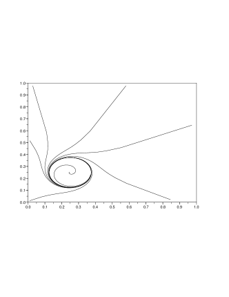
Figure 8: An ordinary differential equation with a limit cycle

whose phase portrait is given in Figure 8. The circle $\mathcal{C}$ centered at $1/4$ with radius $1/8$ is a stable limit set: trajectories spiral into it as time approaches infinity. More precisely, it can be checked that any point in $[0,1]^{2}$ is attracted by $\mathcal{C}$. Moreover, the vector field on the axis is pointing inside the first quadrant, and, for $\ell\in[1,2]$, the vector field on the sloping side $|x|_{1}=\ell$ is pointing inside the domain $G$.

Obviously, the reason for the existence of the limit cycle is that the vector field is the superposition of

$$h_{1}(x)=\left(\begin{array}[]{cc}0&-1\\ 1&0\end{array}\right)\Big{(}x-\frac{1}{4}{\bf 1}\Big{)}$$ (6.69)

– a rotation around the center $(1/4)\bf 1$ which preserves the norm of the vector $(x-(1/4){\bf 1})$–, and of

$$h_{2}(x)=\frac{1}{2}\big{[}1-64\times|x-\frac{1}{4}{\bf 1}|^{2}\big{]}\Big{(}x-\frac{1}{4}{\bf 1}\Big{)}$$ (6.70)

– whose effect is moving the system on the radius issued at the center towards the intersection of the radius and the circle $\mathcal{C}$– . It is plain to check that the components of $h_{1},h_{2}$ are bounded on $[0,1]^{2}$ by a constant strictly smaller than 32. Let $E=\{1,2\}$, and assume that $\mu$ is the Bernoulli law $\mu(1)=\mu(2)=1/2$. With $h^{(1)},h^{(2)}$ the components of $h\in\mathbb{R}^{2}$, define the transition by

$$p(x,i,v)=\left\{\begin{array}[]{cc}\frac{1}{4}\big{(}1\pm\frac{1}{32}h_{i}^{(1)}(x)\big{)}&{\rm for\ }v=\pm e_{1}\\ \frac{1}{4}\big{(}1\pm\frac{1}{32}h_{i}^{(2)}(x)\big{)}&{\rm for\ }v=\pm e_{2}\end{array}\right.\quad,\qquad i=1,2$$ (6.71)

Since $\mu$ is Bernoulli, the limit ordinary differential equation (3.2) is given here by

$$\bar{f}(x)=\frac{1}{128}h(x)$$

with $h$ from (6.68). Assumptions (A.1–3) are fulfilled, as well as the counterpart to (A.4) – with the attractor $\mathcal{C}$ replacing the stable fixed point $0$. Most of the results of Section 4 can be generalized to this case, with the quasi-potential computed as the minimal action over all paths from ${\mathcal{C}}$ to the current point. For instance, (4.13) becomes

$${\mathbb{E}}_{x_{m}}[\tau^{(m)}]=\exp\bigl{[}m(\hat{V}+o(1))\bigr{]}$$

for any sequence $x_{m}\rightarrow x\in G$, with

$$\hat{V}=\inf\{J_{0,T}(\phi);\,\phi_{0}\in{\mathcal{C}},\,|\phi_{T}|_{1}=\ell,\,T>0\}\;.$$

We cannot compute the exact value of the quasi-potential in this example, but it could be estimated numerically from above. Following [16, Chapter 5, Theorem 4.3], we could also provide a suitable version of Proposition 4.19.

7 Appendix A

7.1 Proof of Lemma 4.10: successful coupling

The proof relies on a tricky coupling argument. In [30], the authors investigate the large deviations for stochastic differential equations with a small noise: the coupling argument then follows from standard arguments for the Brownian motion. In our own setting, the standard stochastic analysis tools are useless and we need to construct a coupling for our purpose.

Coupling. For an initial condition $x\in{\mathbb{Z}}^{d}$, $|x|_{1}<\delta m$, the position of the walker is given by

$$X_{n+1}=(2\Pi^{(m)}-{\rm Id})\bigl{(}X_{n}+f(X_{n}/m,\xi_{n},U_{n})\bigr{)},$$

with $X_{0}=x$. Here, $f(z,i,\cdot)$ denotes a function from $(0,1)$ to ${\mathcal{V}}$ such that $f(z,i,U)$ has $p(z,i,\cdot)$ as distribution (typically, $f(z,i,\cdot)$ is an inverse of the cumulative distribution function of $p(z,i,\cdot))$. For another initial condition $y\in{\mathbb{Z}}^{d}$, $|y|_{1}<\delta m$, the position of the walker can be defined in a similar way. The realizations $(U_{n})_{n\geq 0}$ may be the same. Nevertheless, the position may be defined with a different sample of uniform law. It may be also defined with the same sample but with a different function $f$.

In what follows, we are seeking for a copy $(\hat{X}_{n})_{n\geq 0}$ of the walk, starting from $y$, such that $\hat{X}$ and $X$ join up in a finite time. For this purpose, we assume $|x-y|_{1}\in 2{\mathbb{N}}$ (otherwise, it is impossible). We will use the same sample of uniform law but a different function $f$. We thus write

$$\hat{X}_{n+1}=(2\Pi^{(m)}-{\rm Id})\bigl{(}\hat{X}_{n}+\hat{f}_{n}(U_{n})\bigr{)},$$

where $\hat{f}_{n}$ is some random function from $(0,1)$ into ${\mathcal{V}}$, depending on $X_{n}$, $\hat{X}_{n}$ and $\xi_{n}$ such that the conditional law of $\hat{f}_{n}(U_{n})$ with respect to $(X_{n},\hat{X}_{n},\xi_{n})$ is exactly $p(\hat{X}_{n},\xi_{n},\cdot)$. The explicit form of $\hat{f}_{n}$ has to be determined.

To simplify, we will just denote (when possible) $\hat{f}_{n}(U_{n})$ by $\hat{f}_{n}$. Similarly, we will denote $f(X_{n}/m,\xi_{n},U_{n})$ by $f_{n}$ (or $f_{n}(U_{n})$ when necessary).

Before providing an explicit form for $\hat{f}_{n}$, we investigate the $L^{1}$-distance $\Delta_{n}=|X_{n}-\hat{X}_{n}|_{1}$. Loosely speaking, we want it to decrease with $n$. We thus compute $\Delta_{n+1}$ in terms of $\Delta_{n}$. For this purpose, it is crucial to note that $\Delta_{n}$ is always even (because of the particular choice for the initial conditions and for the reflection). We also recall the formula

$$\forall a,b\in\mathbb{R},\ |a+b|=|a|+|b|-2(|a|\wedge|b|){\mathbf{1}}_{\{ab<0\}}.$$

If $X_{n}$ and $\hat{X}_{n}$ are not on the boundary, we deduce

$$|\Delta_{n+1}|_{1}=|\Delta_{n}|_{1}+|f_{n}-\hat{f}_{n}|_{1}-2\sum_{i=1}^{d}[|(\Delta_{n})_{i}|\wedge|(f_{n})_{i}-(\hat{f}_{n})_{i}|]{\mathbf{1}}_{\{(\Delta_{n})_{i}((f_{n})_{i}-(\hat{f}_{n})_{i})<0\}}.$$ (7.1)

If one of the two processes is on the boundary at time $n$, the difference $|\Delta_{n+1}|_{1}-|\Delta_{n}|_{1}$ has the form $|\Delta_{n}+g_{n}-\hat{g}_{n}|_{1}-|\Delta_{n}|_{1}$ with $g_{n}$ and $\hat{g}_{n}$ as in (2.3). We can check that it is always bounded by $|\Delta_{n}+f_{n}-\hat{f}_{n}|_{1}-|\Delta_{n}|_{1}$. In other words, we can forget the reflection. To prove this assertion, it is sufficient to focus on each coordinate. If $(X_{n})_{i}=0$ and $(\hat{X}_{n})_{i}\geq 2$, the proof is obvious. If $(X_{n})_{i}=0$ and $(\hat{X}_{n})_{i}=1$, the proof is the same except for $(\hat{X}_{n+1})_{i}=0$ and $(X_{n})_{i+1}=1$. In this case, the processes switch. However, the result is still true. Other cases are treated in a similar way. Hence, in any case, (7.1) is true with $\leq$ instead of $=$.

Turn back to (7.1). Again, $|f_{n}-\hat{f}_{n}|_{1}$ is always equal to 2, except for $f_{n}=\hat{f}_{n}$. To handle the last term, we introduce the following notations

$$E^{+}_{n}({\rm resp.}\ E^{-}_{n},\ {\rm resp.}\ E^{0}_{n})=\{u\in{\mathcal{V}}:\,\langle\Delta_{n},u\rangle>0\ ({\rm resp.}<0,\ {\rm resp.}=0)\}.$$

If $f_{n}=-\hat{f}_{n}\in E_{n}^{-}$, the sum is equal to $\min(|\langle\Delta_{n},f_{n}\rangle|,2)$. If $f_{n}=\hat{f}_{n}$ or $f_{n}=-\hat{f}_{n}\in E_{n}^{+}\cup E_{n}^{0}$, the sum is zero. If $f_{n}\perp\hat{f}_{n}$, $|(f_{n})_{i}-(\hat{f}_{n})_{i}|$ is 0 or 1 and $(|(\Delta_{n})_{i}|\wedge|(f_{n})_{i}-(\hat{f}_{n})_{i}|){\mathbf{1}}_{\{(\Delta_{n})_{i}((f_{n})_{i}-(\hat{f}_{n})_{i})<0\}}=|(f_{n})_{i}-(\hat{f}_{n})_{i}|{\mathbf{1}}_{\{(\Delta_{n})_{i}((f_{n})_{i}-(\hat{f}_{n})_{i})<0\}}$ is also 0 or 1: it is equal to 1 if and only if $f_{n}\in E_{n}^{-}$ and $i$ is the coordinate of $f_{n}$ or $\hat{f}_{n}\in E_{n}^{+}$ and $i$ is the coordinate of $\hat{f}_{n}$. Hence,

$$\begin{split}|\Delta_{n+1}|_{1}&\leq|\Delta_{n}|_{1}+2-2{\mathbf{1}}_{\{f_{n}=\hat{f}_{n}\}}-2{\mathbf{1}}_{\{f_{n}\perp\hat{f}_{n}\}}\bigl{(}{\mathbf{1}}_{\{f_{n}\in E_{n}^{-}\}}+{\mathbf{1}}_{\{\hat{f}_{n}\in E_{n}^{+}\}}\bigr{)}\\ &\hskip 15.0pt-2[|\langle\Delta_{n},f_{n}\rangle|\wedge 2]{\mathbf{1}}_{\{f_{n}=-\hat{f}_{n},f_{n}\in E_{n}^{-}\}}.\end{split}$$

Noting that $\{f_{n}\perp\hat{f_{n}}\}$ is the complementary of $\{f_{n}=\hat{f}_{n}\}\cup\{f_{n}=-\hat{f}_{n}\}$, we have

$$\begin{split}|\Delta_{n+1}|_{1}&\leq|\Delta_{n}|_{1}+2-2{\mathbf{1}}_{\{f_{n}=\hat{f}_{n}\}}-2\bigl{(}{\mathbf{1}}_{\{f_{n}\in E_{n}^{-}\}}+{\mathbf{1}}_{\{\hat{f}_{n}\in E_{n}^{+}\}}\bigr{)}\\ &\hskip 15.0pt+2\bigl{(}{\mathbf{1}}_{\{f_{n}\in E_{n}^{-}\}}+{\mathbf{1}}_{\{\hat{f}_{n}\in E_{n}^{+}\}}\bigr{)}\bigl{(}{\mathbf{1}}_{\{f_{n}=\hat{f}_{n}\}}+{\mathbf{1}}_{\{f_{n}=-\hat{f}_{n}\}}\bigr{)}\\ &\hskip 15.0pt-2[|\langle\Delta_{n},f_{n}\rangle|\wedge 2]{\mathbf{1}}_{\{f_{n}=-\hat{f}_{n},f_{n}\in E_{n}^{-}\}}.\end{split}$$

We have $\{f_{n}=\hat{f}_{n}\}=\{f_{n}=\hat{f}_{n}\in E_{n}^{+}\}\cup\{f_{n}=\hat{f}_{n}\in E_{n}^{-}\}\cup\{f_{n}=\hat{f}_{n}\in E_{n}^{0}\}$. Moreover $\{f_{n}=-\hat{f}_{n}\in E_{n}^{-}\}=\{\hat{f}_{n}=-f_{n}\in E_{n}^{+}\}$. Hence,

$$\begin{split}|\Delta_{n+1}|_{1}&\leq|\Delta_{n}|_{1}+2-2{\mathbf{1}}_{\{f_{n}=\hat{f}_{n}\in E_{n}^{0}\}}-2\bigl{(}{\mathbf{1}}_{\{f_{n}\in E_{n}^{-}\}}+{\mathbf{1}}_{\{\hat{f}_{n}\in E_{n}^{+}\}}\bigr{)}\\ &\hskip 15.0pt+4{\mathbf{1}}_{\{f_{n}=-\hat{f}_{n},f_{n}\in E_{n}^{-}\}}-2[|\langle\Delta_{n},f_{n}\rangle|\wedge 2]{\mathbf{1}}_{\{f_{n}=-\hat{f}_{n},f_{n}\in E_{n}^{-}\}}.\end{split}$$

Finally,

$$\begin{split}|\Delta_{n+1}|_{1}&\leq|\Delta_{n}|_{1}+2{\mathbf{1}}_{\{f_{n}\in E_{n}^{+}\}}-2{\mathbf{1}}_{\{\hat{f}_{n}\in E_{n}^{+}\}}+2{\mathbf{1}}_{\{f_{n}\in E_{n}^{0},f_{n}\not=\hat{f}_{n}\}}\\ &\hskip 15.0pt+2{\mathbf{1}}_{\{f_{n}=-\hat{f}_{n},f_{n}\in E_{n}^{-}\}}{\mathbf{1}}_{\{|\langle\Delta_{n},f_{n}\rangle|=1\}}.\end{split}$$ (7.2)

We claim that, for $n<\sigma=\inf\{k\geq 0:\,|\Delta_{k}|_{1}=0\}\wedge\inf\{k\geq 0:\,|\Delta_{k}|_{1}>2\lfloor m\delta^{1/2}\rfloor\}$ ($\delta$ small enough), we can choose $\hat{f}_{n}$ such that $\{f_{n}=-\hat{f}_{n},f_{n}\in E_{n}^{-},|\langle\Delta_{n},f_{n}\rangle|=1\}$ is empty and such that ${\mathbb{P}}\{f_{n}\in E_{n}^{0},f_{n}\not=\hat{f}_{n}|\,|{\mathcal{F}}_{n}\}\leq\sum_{u\in E_{n}^{0}}[p(X_{n},\xi_{n},u)-p(\hat{X}_{n},\xi_{n},u)]^{+}$, with ${\mathcal{F}}_{n}={\mathcal{F}}_{n}^{\xi,X,\hat{X}}$.

The idea is the following. We define the random sets (i.e. they may depend on $\xi_{n}$, $X_{n}$ and $\hat{X}_{n}$): $A_{n}(u)=\{r\in(0,1):\,f_{n}(r)=u\}$ and $\hat{A}_{n}(u)=\{r\in(0,1):\,\hat{f}_{n}(r)=u\}$ for $u\in{\mathcal{V}}$. The Lebesgue measures of these sets are known: $|A_{n}(u)|=p(X_{n},\xi_{n},u)$ and $|\hat{A}_{n}(u)|=p(\hat{X}_{n},\xi_{n},u)$. In the sequel, we just write $p_{n}(u)$ and $\hat{p}_{n}(u)$ for these quantities.

For each $u\in{\mathcal{V}}$, $A_{n}(u)$ is an interval (because of the construction by inversion of the cumulative distribution function). However, the geometry of $\hat{A}_{n}(u)$ is free: we will perform the coupling by choosing the form of each $\hat{A}_{n}(u)$ in a suitable way. Without loss of generality, we can assume that $\cup_{u\in E_{n}^{0}}A_{n}(u)$ is an interval with 0 as left bound (see Figure 9).

For $u\in E_{n}^{0}$, we can find a subinterval of $A_{n}(u)$ of length $p_{n}(u)\wedge\hat{p}_{n}(u)$, with the same left bound as $A_{n}(u)$, and set for $r$ in this interval $\hat{f}_{n}(r)=u$. Hence, ${\mathbb{P}}\{f_{n}=u,\hat{f}_{n}\not=u|{\mathcal{F}}_{n}\}\leq(p_{n}(u)-\hat{p}_{n}(u))^{+}$, so that

$${\mathbb{P}}\{f_{n}\in E_{n}^{0},f_{n}\not=\hat{f}_{n}|{\mathcal{F}}_{n}\}\leq\sum_{u\in E_{n}^{0}}[p(X_{n},\xi_{n},u)-p(\hat{X}_{n},\xi_{n},u)]^{+}.$$ (7.3)

This is exactly what we were seeking for.

It remains to choose $\hat{f}_{n}$ such that $\{f_{n}=-\hat{f}_{n},f_{n}\in E_{n}^{-},|\langle\Delta_{n},f_{n}\rangle|=1\}$ is empty. For $n<\sigma$, $\Delta_{n}\not=0$ and $E_{n}^{+}$ cannot be empty. Since $|\Delta_{n}|_{1}$ is always even, $E^{+}_{n}$ cannot count one single vector such that $|\langle\Delta_{n},u\rangle|$ is odd. Hence, the set $\{u\in{\mathcal{V}}:\,|\langle\Delta_{n},u\rangle|\in 2{\mathbb{N}}+1\}$ counts either zero element or more than two. If $M=|E_{n}^{+}|=1$, the set $\{u\in{\mathcal{V}}:\,|\langle\Delta_{n},u\rangle|\in 2{\mathbb{N}}+1\}$ is empty and there is nothing to do. If $M\geq 2$, we can index $E_{n}^{+}$ under the form $E_{n}^{+}=\{v_{1},\dots,v_{M}\}$ with $p_{n}(v_{1})\geq p_{n}(v_{2})\geq\dots\geq p_{n}(v_{M})$. Then, we can assume that the partition related to $f_{n}$ is ordered as follows:

$$\forall u\in E_{n}^{0},\ A_{n}(u)\prec A_{n}(-v_{1})\prec A_{n}(v_{1})\prec A_{n}(-v_{2})\prec A_{n}(v_{2})\dots\prec A_{n}(-v_{M})\prec A_{n}(v_{M}),$$

where $B_{1}\prec B_{2}$ means $\forall(x,y)\in B_{1}\times B_{2},\ x<y$, $B_{1}$ and $B_{2}$ being two subsets of $[0,1]^{2}$ (see Figure 9).

\psfrag{0}{$0$}\psfrag{1}{$1$}\psfrag{en0}{$E_{n}^{0}$}\psfrag{-v1}{$-v_{1}$}\psfrag{-v2}{$-v_{2}$}\psfrag{-v3}{$-v_{3}$}\psfrag{v1}{$v_{1}$}\psfrag{v2}{$v_{2}$}\psfrag{v3}{$v_{3}$}\includegraphics[width=216.81pt,angle={0}]{coupling.eps}

Figure 9: Order for $f_{n}$, $M=3$.

For $\hat{f}_{n}$, we already know that $\hat{A}_{n}(u)$ intersects, for $u\in E_{n}^{0}$, $A_{n}(u)$ on an interval of length $p_{n}(u)\wedge\hat{p}_{n}(u)$. Then, we can complete $\hat{A}_{n}(u)$, if necessary, that is if $\hat{p}_{n}(u)>p_{n}(u)$, so that $\cup_{u\in E_{n}^{0}}\hat{A}_{n}(u)$ is an interval with zero as lower bound (see Figure 10). In particular, we have

$$\forall u\in E_{n}^{0},\ \forall v\not\in E_{n}^{0},\ \hat{A}_{n}(u)\prec\hat{A}_{n}(v).$$

Then, we can complete the partition associated to $\hat{f}_{n}$ as follows

$$\hat{A}_{n}(v_{2})\prec\hat{A}_{n}(-v_{2})\prec\hat{A}_{n}(v_{3})\prec\hat{A}_{n}(-v_{3})\dots\prec\tilde{A}_{n}(v_{M})\prec\hat{A}_{n}(-v_{M})\prec\hat{A}_{n}(-v_{1})\prec\hat{A}_{n}(v_{1}),$$

see Figure 10.

\psfrag{0}{$0$}\psfrag{1}{$1$}\psfrag{en0}{$E_{n}^{0}$}\psfrag{-v1}{$-v_{1}$}\psfrag{-v2}{$-v_{2}$}\psfrag{-v3}{$-v_{3}$}\psfrag{v1}{$v_{1}$}\psfrag{v2}{$v_{2}$}\psfrag{v3}{$v_{3}$}\includegraphics[width=216.81pt,angle={0}]{coupling2.eps}

Figure 10: Order for $\hat{f}_{n}$, $M=3$.

We now prove that, for $\delta$ small enough and $u\in E_{n}^{-}$, the sets $A_{n}(u)$ and $\hat{A}_{n}(-u)$ are disjoint. For $2\leq i\leq M$, the right boundary of $\hat{A}_{n}(v_{i})$ is given by $\hat{p}_{n}(E_{n}^{0})+\hat{p}_{n}(v_{2})+\hat{p}_{n}(-v_{2})+\dots+\hat{p}_{n}(v_{i})$ and the left boundary of $A_{n}(-v_{i})$ is given by $p_{n}(E_{n}^{0})+p_{n}(-v_{1})+p_{n}(v_{1})+\dots+p_{n}(-v_{i-1})+p_{n}(v_{i-1})$. By the Lipschitz property of $p$, the difference between $p_{n}(u)$ and $\hat{p}_{n}(u)$ is bounded by $(C/m)|X_{n}-\hat{X}_{n}|_{1}\leq 2C\delta^{1/2}$ for every $u\in{\mathcal{V}}$. Since $p_{n}(v_{1})\geq p_{n}(v_{i})$, we have

$$\begin{split}&p_{n}(E_{n}^{0})+p_{n}(-v_{1})+p_{n}(v_{1})+\dots+p_{n}(-v_{i-1})+p_{n}(v_{i-1})\\ &\geq\hat{p}_{n}(E^{n}_{0})+\hat{p}_{n}(-v_{2})+\hat{p}_{n}(v_{2})+\dots+\hat{p}_{n}(-v_{i-1})+\hat{p}_{n}(v_{i-1})+\hat{p}_{n}(v_{i})+p_{n}(-v_{1})-4Cd\delta^{1/2}\\ &\geq\hat{p}_{n}(E^{n}_{0})+\hat{p}_{n}(-v_{2})+\hat{p}_{n}(v_{2})+\dots+\hat{p}_{n}(-v_{i-1})+\hat{p}_{n}(v_{i-1})+\hat{p}_{n}(v_{i})+c-4Cd\delta^{1/2},\end{split}$$

with $c=\inf\{p(z,i,v);\,z\in[0,1]^{d},\,i\in E,\,v\in{\mathcal{V}}\}>0$ (see Assumption (A.2)). For $\delta$ small enough, we obtain $\hat{A}_{n}(v_{i})\cap A_{n}(-v_{i})=\emptyset$. It remains to prove the same thing for $i=1$. The right boundary of $A_{n}(-v_{1})$ is given by $p_{n}(E_{n}^{0})+p_{n}(-v_{1})$ and the left boundary of $\hat{A}_{n}(v_{1})$ is given by $\hat{p}_{n}(E_{n}^{0})+\hat{p}_{n}(v_{2})+\hat{p}_{n}(-v_{2})+\dots+\hat{p}_{n}(v_{M})+\hat{p}_{n}(-v_{M})+\hat{p}_{n}(-v_{1})\geq p_{n}(E_{n}^{0})+p_{n}(-v_{1})+2c-4Cd\delta^{1/2}$. This completes the construction of $\hat{f}_{n}$ for $M\geq 2$.

Hitting Time. Recall that ${\mathcal{F}}_{n}={\mathcal{F}}_{n}^{\xi,X,\hat{X}}$ for all $n\geq 0$. By (7.2) and (7.3), we have for $\delta$ small enough (say $\delta\leq\rho_{0}$ for some $\rho_{0}>0$) and $n<\sigma$

$${\mathbb{E}}\bigl{[}|\Delta_{n+1}|_{1}|{\mathcal{F}}_{n}\bigr{]}-|\Delta_{n}|_{1}\leq 2(p_{n}-\hat{p}_{n})^{+}(E_{n}^{0})+2p_{n}(E_{n}^{+})-2\hat{p}_{n}(E_{n}^{+}),$$ (7.4)

where $(p_{n}(\cdot)-\hat{p}_{n}(\cdot))^{+}(A)=\sum_{u\in A}(p_{n}(u)-\hat{p}_{n}(u))^{+}$ for any subset $A$ of ${\mathcal{V}}$ (the same holds for $p_{n}(A)$ and $\hat{p}_{n}(A)$). By (4.22) in Theorem 4.9, we have

$$\begin{split}&2(p_{n}-\hat{p}_{n})^{+}(E_{n}^{0})+2p_{n}(E_{n}^{+})-2\hat{p}_{n}(E_{n}^{+})\\ &=2(p_{n}-\hat{p}_{n})^{+}(E_{n}^{0})+p_{n}(E^{+}_{n})-\hat{p}_{n}(E_{n}^{+})\\ &\hskip 15.0pt+\bigl{(}1-p_{n}(E^{0}_{n})-p_{n}(E^{-}_{n})\bigr{)}-\bigl{(}1-\hat{p}_{n}(E^{0}_{n})-\hat{p}_{n}(E^{-}_{n})\bigr{)}\\ &=2(p_{n}-\hat{p}_{n})^{+}(E_{n}^{0})-(p_{n}-\hat{p}_{n})(E_{n}^{0})+(p_{n}-\hat{p}_{n})(E_{n}^{+})-(p_{n}-\hat{p}_{n})(E_{n}^{-})\\ &=\sum_{u\in\Lambda,u\perp\Delta_{n}}|p_{n}(u)-\hat{p}_{n}(u)|+\sum_{u\in\Lambda}\bigl{(}p_{n}(u)-\hat{p}_{n}(u)\bigr{)}{\rm sgn}\bigl{(}\langle\Delta_{n},u\rangle\bigr{)}\\ &\leq-(\kappa/m)|\Delta_{n}|_{1}.\end{split}$$

By (7.4), we can write $|\Delta_{n+1}|_{1}=|\Delta_{n}|_{1}+2\varepsilon_{n+1}$, with $\varepsilon_{n}\in\{-1,0,1\}$ and ${\mathbb{E}}(2\varepsilon_{n+1}|{\mathcal{F}}_{n})\leq-(\kappa/m)|\Delta_{n}|_{1}$ for $n<\sigma$. Hence, ${\mathbb{E}}(|\Delta_{n+1}|_{1}|{\mathcal{F}}_{n})\leq(1-\kappa/m)|\Delta_{n}|_{1}$ for $n<\sigma$, so that $((1-\kappa/m)^{-n\wedge\sigma}|\Delta_{n\wedge\sigma}|_{1})_{n\geq 0}$ is a supermartingale. We deduce that, for all $n\geq 1$,

$$2{\mathbb{P}}\{\sigma>n\}(1-\kappa/m)^{-n}\leq{\mathbb{E}}[(1-\kappa/m)^{-\sigma\wedge n}|\Delta_{\sigma\wedge n}|_{1}]\leq 2\delta m.$$

We obtain

$${\mathbb{E}}(\sigma)\leq\delta m\sum_{n\geq 0}(1-\kappa/m)^{n}\leq C^{\prime}\delta m^{2},$$ (7.5)

for some constant $C^{\prime}>0$.

We now investigate ${\mathbb{P}}\{|\Delta_{\sigma}|_{1}>2\lfloor m\delta^{1/2}\rfloor\}$. Since $((1-\kappa/m)^{-n\wedge\sigma}|\Delta_{n\wedge\sigma}|_{1})_{n\geq 0}$ is a supermartingale, we have for all $n\geq m^{3/2}$,

$$(1-\kappa/m)^{-m^{3/2}}{\mathbb{E}}\bigl{[}{\mathbf{1}}_{\{\sigma\geq m^{3/2}\}}|\Delta_{\sigma\wedge n}|_{1}\bigr{]}\leq{\mathbb{E}}\bigl{[}(1-\kappa/m)^{-\sigma\wedge n}|\Delta_{\sigma\wedge n}|_{1}\bigr{]}\leq 2\delta m.$$

Letting $n$ tend to $+\infty$, we deduce (changing if necessary the value of $C^{\prime}$)

$$(1-\kappa/m)^{-m^{3/2}}{\mathbb{P}}\bigl{\{}\sigma\geq m^{3/2},|\Delta_{\sigma}|_{1}>2\lfloor m\delta^{1/2}\rfloor\bigr{\}}\leq C^{\prime}.$$ (7.6)

It remains to see what happens for $\sigma<m^{3/2}$. We set $q_{n}^{+}={\mathbb{P}}\{\varepsilon_{n}=1|{\mathcal{F}}_{n}\}$ and $q_{n}^{-}={\mathbb{P}}\{\varepsilon_{n}=-1|{\mathcal{F}}_{n}\}$. Conditionally to the past, the process $(|\Delta_{k}|_{1})_{k\geq 0}$ doesn’t move at time $n$ with probability $1-(q_{n}^{+}+q_{n}^{-})$. Conditionally to moving, it jumps with probabilities $q_{n}^{+}/(q_{n}^{+}+q_{n}^{-})$ and $q_{n}^{-}/(q_{n}^{+}+q_{n}^{-})$. Since ${\mathbb{E}}(\varepsilon_{n+1}|{\mathcal{F}}_{n})<0$, we have $q_{n}^{+}/(q_{n}^{+}+q_{n}^{-})<1/2$. Hence, the time needed by the chain $(|\Delta_{n}|_{1})_{n\geq 0}$ to reach $2\lfloor m\delta^{1/2}\rfloor$ is (stochastically) larger than the time needed by the simple random walk to hit $2\lfloor m\delta^{1/2}\rfloor-2\lfloor m\delta\rfloor$ when starting from zero. Hence,

$${\mathbb{P}}\bigl{\{}\sigma<m^{3/2},|\Delta_{\sigma}|_{1}>2\lfloor m\delta^{1/2}\rfloor\bigr{\}}\leq{\mathbb{P}}\{\tau_{2\lfloor m\delta^{1/2}\rfloor-2\lfloor m\delta\rfloor}<m^{3/2}\},$$

where $\tau_{L}$ denotes the hitting time, by the simple random walk, of a given integer $L$. It is well known (see e.g. [31, Chapter 10]) that ${\mathbb{P}}\{\tau_{L}\leq m^{3/2}\}\leq\exp(-\alpha L+m^{3/2}\ln(\cosh(\alpha)))$ for any $\alpha>0$. Choosing $\alpha=m^{-3/4}$, we have ${\mathbb{P}}\{\tau_{L}\leq m^{3/2}\}\leq\exp(-Lm^{-3/4}+m^{3/2}\ln(\cosh(m^{-3/4})))$. If $L=\eta m$, for some $\eta>0$, ${\mathbb{P}}\{\tau_{\eta m}\leq m^{3/2}\}\leq C^{\prime}\exp(-\eta m^{1/4})$. Hence (changing $C^{\prime}$ if necessary),

$${\mathbb{P}}\bigl{\{}\sigma<m^{3/2},|\Delta_{\sigma}|_{1}>2\lfloor m\delta^{1/2}\rfloor\bigr{\}}\leq C^{\prime}\exp(-2(\delta^{1/2}-\delta)m^{1/4}).$$ (7.7)

We can complete the proof of Lemma 4.10. We have, for all $t\geq S$,

$$|{\mathbb{P}}_{x}\{\tau^{(m)}>m^{2}t\}-{\mathbb{P}}_{y}\{\tau^{(m)}>m^{2}t\}|\leq 2\mathbb{P}\{\sigma>m^{3}S\ {\rm or}\ |\Delta_{\sigma}|\not=0\}.$$

By (7.5), $\mathbb{P}\{\sigma>m^{3}S\}\leq C^{\prime}\delta S^{-1}m^{-1}$. By (7.6) and (7.7), $\mathbb{P}\{|\Delta_{\sigma}|\not=0\}\leq C^{\prime}[\exp(-2(\delta^{1/2}-\delta)m^{1/4})+\exp(-\kappa m^{1/2})]$. This completes the proof.

7.2 Proof of Lemma 4.20

For a given $x\in[0,1]^{d}$, we have to prove that the bilinear form $\nabla^{2}_{\alpha,\alpha}H:\lambda\in\mathbb{R}^{d}\mapsto\sum_{i,j}\lambda_{i}\lambda_{j}[\partial^{2}H/\partial\alpha_{i}\partial\alpha_{j}](x,0)$ is positive definite. We first note that the bilinear form ${\mathcal{E}}_{f}:\lambda\in\mathbb{R}^{d}\mapsto\sum_{i,j=1}^{d}\sum_{k\in E}\mu(k)\lambda_{i}\lambda_{j}({\mathbb{E}}[(f_{i}f_{j})(x,k,U)]-{\mathbb{E}}[f_{i}(x,k,U)]{\mathbb{E}}[f_{j}(x,k,U)])$ induced by the averaged covariance matrix of the random vectors $f(x,k,U)$ ($U$ following the uniform distribution on $(0,1)$) is nondegenerate. Indeed, for all $\lambda\in\mathbb{R}^{d}$, Jensen’s inequality yields

$$\begin{split}{\mathcal{E}}_{f}(\lambda)&=\sum_{i=1}^{d}\sum_{k\in E}\mu(k)\lambda_{i}^{2}{\mathbb{E}}(f_{i}^{2}(x,k,U))-\sum_{k\in E}\mu(k)\bigl{(}\sum_{i=1}^{d}\lambda_{i}{\mathbb{E}}(f_{i}(x,k,U))\bigr{)}^{2}\\ &=\sum_{i=1}^{d}\sum_{k\in E}\lambda_{i}^{2}\mu(k)p(x,k,\pm e_{i})-\sum_{k\in E}\mu(k)\bigl{(}\sum_{i=1}^{d}\lambda_{i}[p(x,k,e_{i})-p(x,k,-e_{i})]\bigr{)}^{2}\\ &\geq\sum_{i=1}^{d}\sum_{k\in E}\lambda_{i}^{2}\mu(k)p(x,k,\pm e_{i})-\sum_{i=1}^{d}\sum_{k\in E}\mu(k)\lambda_{i}^{2}\frac{[p(x,k,e_{i})-p(x,k,-e_{i})]^{2}}{p(x,k,\pm e_{i})}\\ &=\sum_{i=1}^{d}\sum_{k\in E}\lambda_{i}^{2}\mu(k)\frac{4p(x,k,e_{i})p(x,k,-e_{i})}{p(x,k,\pm e_{i})}>0,\end{split}$$

with $p(x,k,\pm e_{i})=p(x,k,e_{i})+p(x,k,-e_{i})$. In what follows, we provide an explicit expression for $\nabla^{2}_{\alpha,\alpha}H$ and then compare it to ${\mathcal{E}}_{f}$. We know that the leading eigenvalue of the matrix $Q(x,\alpha)$ (see (3.4)) is simple and equal to $\exp(H(x,\alpha))$. As a by-product, the coordinates of the corresponding eigenvector $v(x,\alpha)$ (i.e. of the $\ell^{1}$ normalized eigenvector with positive entries) are infinitely differentiable with respect to $\alpha$. In particular, we can differentiate twice the relationship $Q(x,\alpha)v(x,\alpha)=\exp(H(x,\alpha))v(x,\alpha)$ with respect to $\alpha_{i},\alpha_{j}$. We obtain

$$\begin{split}&\bigl{[}\frac{\partial Q}{\partial\alpha_{i}}v+Q\frac{\partial v}{\partial\alpha_{i}}\bigr{]}(x,\alpha)=\bigl{[}\bigl{(}\frac{\partial H}{\partial\alpha_{i}}v+\frac{\partial v}{\partial\alpha_{i}}\bigr{)}\exp(H)\bigr{]}(x,\alpha)\\ &\bigl{[}\frac{\partial^{2}Q}{\partial\alpha_{i}\alpha_{j}}v+\frac{\partial Q}{\partial\alpha_{i}}\frac{\partial v}{\partial\alpha_{j}}+\frac{\partial Q}{\partial\alpha_{j}}\frac{\partial v}{\partial\alpha_{i}}+Q\frac{\partial^{2}v}{\partial\alpha_{i}\partial\alpha_{j}}\bigr{]}(x,\alpha)\\ &\hskip 5.0pt=\bigl{[}\bigl{(}\frac{\partial^{2}H}{\partial\alpha_{i}\partial\alpha_{j}}v+\frac{\partial H}{\partial\alpha_{i}}\frac{\partial v}{\partial\alpha_{j}}+\frac{\partial H}{\partial\alpha_{i}}\frac{\partial H}{\partial\alpha_{j}}v+\frac{\partial^{2}v}{\partial\alpha_{i}\partial\alpha_{j}}+\frac{\partial v}{\partial\alpha_{i}}\frac{\partial H}{\partial\alpha_{j}}\bigr{)}\exp(H)\bigr{]}(x,\alpha).\end{split}$$

For $\alpha=0$, we know that $Q(x,0)=P$ (so that $v(x,0)={\mathbf{1}}=(1,\dots,1)^{t}$) and $[\partial Q/\partial\alpha_{i}](x,0)=(P_{k,k^{\prime}}{\mathbb{E}}[f_{i}(x,k,U)])_{k,k^{\prime}\in E}$. Hence, for every $k\in E$, ${\mathbb{E}}[f_{i}(x,k,U)]+\sum_{k^{\prime}\in E}P_{k,k^{\prime}}[\partial v_{k^{\prime}}/\partial\alpha_{i}](x,0)=[\partial H/\partial\alpha_{i}](x,0)+[\partial v_{k}/\partial\alpha_{i}](x,0)$. Integrating with respect to the invariant measure $\mu$, we deduce that $[\partial H/\partial\alpha_{i}](x,0)=\sum_{k\in E}\mu(k){\mathbb{E}}[f_{i}(x,k,U)]=\bar{f}_{i}(x)$ . Finally,

$$\sum_{k^{\prime}\in E}({\rm Id}-P)_{k,k^{\prime}}\frac{\partial v_{k^{\prime}}}{\partial\alpha_{i}}(x,0)={\mathbb{E}}[f_{i}(x,k,U)]-\bar{f}_{i}(x).$$ (7.8)

Applying the same method for the second order derivatives, we obtain for every $k\in E$:

$$\begin{split}&{\mathbb{E}}[(f_{i}f_{j})(x,k,U)]+\sum_{k^{\prime}\in E}P_{k,k^{\prime}}\frac{\partial^{2}v_{k^{\prime}}}{\partial\alpha_{i}\partial\alpha_{j}}(x,0)\\ &\hskip 15.0pt+\sum_{k^{\prime}\in E}\bigl{[}{\mathbb{E}}[f_{i}(x,k,U)]P_{k,k^{\prime}}-\bar{f}_{i}(x)\delta_{k,k^{\prime}}\bigr{]}\frac{\partial v_{k^{\prime}}}{\partial\alpha_{j}}(x,0)\\ &\hskip 15.0pt+\sum_{k^{\prime}\in E}\bigl{[}{\mathbb{E}}[f_{j}(x,k,U)]P_{k,k^{\prime}}-\bar{f}_{j}(x)\delta_{k,k^{\prime}}\bigr{]}\frac{\partial v_{k^{\prime}}}{\partial\alpha_{i}}(x,0)\\ &=\frac{\partial^{2}H}{\partial\alpha_{i}\partial\alpha_{j}}(x,0)+[\bar{f}_{i}\bar{f}_{j}](x)+\frac{\partial^{2}v_{k}}{\partial\alpha_{i}\partial\alpha_{j}}(x,0).\end{split}$$ (7.9)

By (7.8), we have

$$\begin{split}&\sum_{k,k^{\prime}\in E}\mu(k)\bigl{[}{\mathbb{E}}[f_{i}(x,k,U)]P_{k,k^{\prime}}-\bar{f}_{i}(x)\delta_{k,k^{\prime}}\bigr{]}\frac{\partial v_{k^{\prime}}}{\partial\alpha_{j}}(x,0)\\ &=\sum_{k,k^{\prime}\in E}\mu(k)\bigl{[}{\mathbb{E}}[f_{i}(x,k,U)]-\bar{f}_{i}(x)\bigr{]}P_{k,k^{\prime}}\frac{\partial v_{k^{\prime}}}{\partial\alpha_{j}}(x,0)\\ &=\sum_{k,k^{\prime},k^{\prime\prime}\in E}\mu(k)({\rm Id}-P)_{k,k^{\prime\prime}}\frac{\partial v_{k^{\prime\prime}}}{\partial\alpha_{i}}(x,0)P_{k,k^{\prime}}\frac{\partial v_{k^{\prime}}}{\partial\alpha_{j}}(x,0)\\ &=\langle({\rm Id}-P)\frac{\partial v}{\partial\alpha_{i}}(x,0),P\frac{\partial v}{\partial\alpha_{j}}(x,0)\rangle_{\mu},\end{split}$$

where $\langle\cdot,\cdot\rangle_{\mu}$ denotes the scalar product on $L^{2}(\mu)$ and ${\rm Id}$ the identity matrix on $E$. We now integrate (7.9) with respect to the invariant measure, we deduce

$$\begin{split}\frac{\partial^{2}H}{\partial\alpha_{i}\partial\alpha_{j}}(x,0)&=\sum_{k\in E}\mu(k){\mathbb{E}}[(f_{i}f_{j})(x,k,U)]-[\bar{f}_{i}\bar{f}_{j}](x)\\ &\hskip 5.0pt+\langle({\rm Id}-P)\frac{\partial v}{\partial\alpha_{i}}(x,0),P\frac{\partial v}{\partial\alpha_{j}}(x,0)\rangle_{\mu}\\ &\hskip 5.0pt+\langle({\rm Id}-P)\frac{\partial v}{\partial\alpha_{j}}(x,0),P\frac{\partial v}{\partial\alpha_{i}}(x,0)\rangle_{\mu}.\end{split}$$ (7.10)

Using (7.8), we deduce

$$\begin{split}&\sum_{k\in E}\mu(k){\mathbb{E}}[f_{i}(x,k,U)]{\mathbb{E}}[f_{j}(x,k,U)]-[\bar{f}_{i}\bar{f}_{j}](x)\\ &\hskip 15.0pt=\langle({\rm Id}-P)\frac{\partial v}{\partial\alpha_{i}}(x,0),({\rm Id}-P)\frac{\partial v}{\partial\alpha_{j}}(x,0)\rangle_{\mu}.\end{split}$$ (7.11)

Plugging (7.11) into (7.10), we obtain

$$\begin{split}\frac{\partial^{2}H}{\partial\alpha_{i}\partial\alpha_{j}}(x,0)&=\sum_{k\in E}\mu(k){\mathbb{E}}[(f_{i}f_{j})(x,k,U)]-\sum_{k\in E}\mu(k){\mathbb{E}}[f_{i}(x,k,U)]{\mathbb{E}}[f_{j}(x,k,U)]\\ &+\langle({\rm Id}-P)\frac{\partial v}{\partial\alpha_{i}}(x,0),({\rm Id}-P)\frac{\partial v}{\partial\alpha_{j}}(x,0)\rangle_{\mu}\\ &+\langle({\rm Id}-P)\frac{\partial v}{\partial\alpha_{i}}(x,0),P\frac{\partial v}{\partial\alpha_{j}}(x,0)\rangle_{\mu}+\langle({\rm Id}-P)\frac{\partial v}{\partial\alpha_{j}}(x,0),P\frac{\partial v}{\partial\alpha_{i}}(x,0)\rangle_{\mu}\end{split}$$

For all $(\lambda_{i})_{1\leq i\leq d}\in\mathbb{R}^{d}$ and $k\in E$, we set $u^{\lambda}(k)=\sum_{i=1}^{d}\lambda_{i}[\partial v_{k}/\partial\alpha_{i}](x,0)$. Then,

$$\begin{split}\nabla^{2}_{\alpha,\alpha}H(\lambda)&={\mathcal{E}}_{f}(\lambda)+\langle({\rm Id}-P)u^{\lambda},(I-P)u^{\lambda}\rangle_{\mu}+2\langle({\rm Id}-P)u^{\lambda},Pu^{\lambda}\rangle_{\mu}.\\ &={\mathcal{E}}_{f}(\lambda)+\langle u^{\lambda},u^{\lambda}\rangle_{\mu}-\langle Pu^{\lambda},Pu^{\lambda}\rangle_{\mu}\\ &={\mathcal{E}}_{f}(\lambda)+\int_{E}d\mu(k){\mathbb{E}}^{k}\bigl{[}(u^{\lambda}(\xi_{1}))^{2}\bigr{]}-\int_{E}d\mu(k)\bigl{[}{\mathbb{E}}^{k}u^{\lambda}(\xi_{1})\bigr{]}^{2}\geq{\mathcal{E}}_{f}(\lambda).\end{split}$$

This completes the proof.

References

• [1] Atar, R., Dupuis, P.: Large deviations and queueing networks: methods for rate function identification. Stochastic Process. Appl. 84 255–296, 1999.
• [2] Azencott, R., Ruget, G.: Mélanges d’équations différentielles et grands écarts à la loi des grands nombres. Z. Wahrscheinlichkeitstheorie und Verw. Gebiete 38 1–54, 1977.
• [3] Azencott, R.: Grandes déviations et applications. In: Eighth Saint Flour Probability Summer School—1978, pp. 1–176, Lecture Notes in Math., 774, Springer, Berlin, 1980.
• [4] Baldi, P.: Large deviations and stochastic homogenization. Ann. Mat. Pura Appl. 151 161–177, 1988.
• [5] Bardi, M., Capuzzo-Dolcetta, I. Optimal control and viscosity solutions of Hamilton-Jacobi-Bellman equations. Birkh user Boston, Inc., Boston, MA, 1997.
• [6] Barles, G. Solutions de viscosité des équations de Hamilton-Jacobi. Springer-Verlag, Paris, 1994.
• [7] Capuzzo-Dolcetta, I., Lions, P.-L. Hamilton-Jacobi equations with state constraints. Trans. Amer. Math. Soc., 318, 643–683, 1990.
• [8] Comets, F., Delarue, F., Schott, R.: Distributed Algorithms in an Ergodic Markovian Environment. Random Structures and Algorithms 30, 131-167, 2007.
• [9] Dembo, A., Zeitouni, O.: Large deviations techniques and applications. Second edition. Applications of Mathematics 38. Springer-Verlag, New York, 1998.
• [10] Dupuis, P.: Large deviations analysis of reflected diffusions and constrained stochastic approximation algorithms in convex sets. Stochastics 21, 63–96, 1987.
• [11] Dupuis, P.: Large deviations analysis of some recursive algorithms with state dependent noise. Ann. Probab. 16, 1509–1536, 1988.
• [12] Dupuis, P. and Ellis, R.S.: The large deviations principle for a general class of queueing systems I. Trans. Amer. Math. Soc. 347 2689–2751, 1995.
• [13] Dupuis, P., Ramanan, K.: A time-reversed representation for the tail probabilities of stationary reflected Brownian motion. Stochastic Process. Appl. 98 253–287, 2002.
• [14] Feng, J., Kurtz T.: Large deviations for stochastic processes, 2005. http://www.math.wisc.edu/ kurtz/feng/ldp.htm
• [15] Flajolet, P.: The evolution of two stacks in bounded space and random walks in a triangle. Proceedings of FCT’86, LNCS 233, 325–340, Springer Verlag, 1986.
• [16] Freidlin, M., Wentzell, A.D.: Random perturbations of dynamical systems. Grundlehren der Mathematischen Wissenschaften, 260. Springer-Verlag, New York, 1984.
• [17] Guillotin-Plantard, N., Schott, R.: Distributed algorithms with dynamic random transitions. Random Structures and Algorithms 21 371–396, 2002.
• [18] Guillotin-Plantard, N., Schott, R.: Dynamic random walks. Theory and applications. Elsevier B.V., Amsterdam, 2006.
• [19] Gulinsky, O., Veretennikov, A.: Large deviations for discrete-time processes with averaging. VSP, Utrecht, 1993.
• [20] Ignatiouk-Robert, I.: Large deviations for processes with discontinuous statistics. Ann. Probab. 33 1479–1508, 2005.
• [21] Ignatiouk-Robert, I.: Sample path large deviations and convergence parameters. Ann. Appl. Probab. 11 1292–1329, 2001.
• [22] Knuth D.E., The art of computer programming, Vol. 1, Addison-Wesley, 1973.
• [23] Lions, P.-L., Sznitman, A.-S.: Stochastic differential equations with reflecting boundary conditions. Comm. Pure Appl. Math. 37 511–537, 1984.
• [24] Lions, P.-L. Neumann type boundary conditions for Hamilton-Jacobi equations. Duke Math. J., 52, 793–820, 1985.
• [25] Lions, P.-L. Optimal control of reflected diffusion processes: an example of state constraints. In: Stochastic differential systems (Bad Honnef, 1985), 269–276, Lecture Notes in Control and Inform. Sci., 78, Springer, Berlin, 1986.
• [26] Louchard, G.: Some distributed algorithms revisited. Commun. Statist. Stochastic Models 4 563–586, 1995.
• [27] Louchard, G., Schott, R.: Probabilistic analysis of some distributed algorithms. Random Structures and Algorithms 2 151–186, 1991.
• [28] Louchard, G., Schott, R., Tolley, M., Zimmermann, P.: Random walks, heat equations and distributed algorithms algorithms. Computat. Appl. Math. 53 243–274, 1994.
• [29] Maier, R.: Colliding stacks: a large deviations analysis. Random Structures Algorithms 2 379–420, 1991.
• [30] Olivieri, E., Vares, M.E.: Large deviations and metastability. Encyclopedia of Mathematics and its Applications, 100. Cambridge University Press, Cambridge, 2005.
• [31] Williams, D.: Probability with Martingales. Cambridge University Press, Cambridge, 1991.
• [32] Yao, A.: An analysis of a memory allocation scheme for implementing stacks. SIAM J. Comput 10 398–403, 1981.