A TFD model for the Electrospheres of Bare Strange Quark Stars

Abstract

We study the layer of electrons on bare strange star surfaces, taking the Dirac exchange-energy into account. Because electrons are fermions, the electron wave function must be of exchange-antisymmetry. The Dirac exchange-energy originates, consequently, from the exchange-antisymmetry of electron wave functions. This consideration may result in changing the electron distribution and the electric field on the surface of bare strange star. The strong magnetic field effect on the structures of the electrospheres is also discussed.

We are unfortunately not certain about the real state of matter in pulsar-like stars even 40 years after the discovery of pulsar. Nuclear matter (neutron stars) is one of the speculations, while quark matter (quark stars) is an alternative (e.g., lp04, ; weber05, ; Alcock, ; Haensel, ; Glendenning, ; Cheng, ; Weber, ; Cheng & Harko, ; Alford & Reddy, ; Lugones & Horvath, ). The observational features could be very similar for normal neutron stars and crusted strange quark stars, but the bare quark surface should be very useful for us to distinguish those two kinds of compact objects Xu07 . It is therefore worth studying the structure of electrospheres of bare strange quark stars in details (for the previous researches, see, e.g., Usov05, ).

If the Witten’s conjecture Witten (the strange quark matter in bulk is the most stable strong interaction system) is correct, strange quark star with almost equal numbers of $u$, $d$, and $s$ quarks would exist in case that the baryon density is higher than the nuclear density. In the strange quark matter, the three flavors of quarks may keep a chemical equilibrium, and the whole of the quarks will be electropositive because of massive $s$ quarks. In order to make sure the strange quark matter is globally electroneutral, there must exist proper quantity of electrons. Xu1

Alcock et al. Alcock thought that (1) a strange quark star would accrete inter-stellar matter, and then a crust would form, wrapping the strange quark star, and (2) a bare strange star can not manifest itself as a radio pulsar because of being unable to generate a magnetosphere. However, it is argued Xu2 ; xu02 ; cyx07 that there are some advantages in understanding the observational features if radio pulsars are bare strange stars and that the circumstellar matter could not be accreted onto the star’s surface at all (i.e., the quark surface keeps bare). The electrons can only extend thousands of femto-meters above the quark surface, and an extremely strong electric field $E\sim 5\times 10^{17}$ V/cm forms Alcock ; Kettner ; Xu1 ; Hu & Xu , being higher than the critical field $E_{\rm cr}\simeq 1.3\times 10^{16}$V/cm Schwinger . It is worth noting that the Usov mechanism ($e^{\pm}$-pair production in degenerate electron gas with strong electric field) Usov1 ; Usov2 ; Aksenov may dominate in the thermal emission of a bare strange star with a surface temperature $T_{\rm s}$, $6\times 10^{8}$ K $\lesssim T_{\rm s}\lesssim 5\times 10^{10}$K.

Sanwal et al. Sanwal discovered two absorption features in 1E 1207-5209’s X-ray spectrum, $0.7$ keV, $1.4$ keV. Based on the works of Ruder et al. Ruder and Mori and Hailey et al. Mori & Hailey , Sanwal et al. thought the two absorption features originated from the atomic transitions of once-ionized helium in the neutron star atmosphere with a strong magnetic field. They do not think it is likely to interpret the two absorption features in terms of electron cyclotron lines for four points of view. Howsoever, these points were criticized by Xu et al. Xu3 , who suggested that the two absorption features could be of electron cyclotron lines from the bare strange quark star surface. Xu et al. proposed a model with a debris disc around a bare strange quark star, which could slow down the spin and decrease the inferred strength of the dipole magnetic field so as to fit the energy differences of Landau levels ($\sim 0.7$ keV). It is then very necessary for us to understand the exact electron distribution on the bare strange star surface in terms of cyclotron lines.

The extreme relativistic electron distribution of the bare strange star surface has been calculated via Thomas-Fermi Model Alcock ; Xu1 , but the Dirac exchange-energy Dreizler was not taken into account up-to-now. The wave function must be of exchange-antisymmetry for fermions, and the Dirac exchange-energy originates consequently. For the Dirac exchange-energy plays an important role in the low-density electrons and make a dramatic effect on the electron distribution, we need to take it into account, applying the Thomas-Fermi-Dirac (TFD) model for bare strange stars.

The theoretical basis of the Thomas-Fermi-Dirac Model is the density functional theory, called DFT for short. Via this theory, we could obtain the Thomas-Fermi-Dirac Equation of the electron density.

In DFT, the ground state energy of the system is the functional of the ground state electron density, which is Dreizler

$$E_{0}=E_{0}[n_{0}(\vec{r})]$$ (1)

where $E_{0}$ is the ground state energy of the system, $n_{0}$ is the ground state electron density. The ground state energy of the electron gas is composed of three parts (we used the different form from ref. Dreizler ),

$$E_{0}[n_{0}(\vec{r})] = -e\int\!n_{0}(\vec{r})V_{0}(\vec{r})\textmd{d}\vec{r}$$ (2)

$$+\langle\Psi_{0}|\frac{1}{2}\sum_{i\neq{j}}\frac{e^{2}}{|\vec{r_{i}}-\vec{r_{j}}|}|\Psi_{0}\rangle$$

$$+\langle\Psi_{0}|\sum_{i}\hat{T}_{i}|\Psi_{0}\rangle,$$

where $|\Psi_{0}\rangle$is the ground state vector of the electron gas, the first term of right side is the outer potential energy of the system, the second term is the inter-electronic Coulomb energy and the last one is the electrons kinetic energy. Here we can divide the inter-electronic Coulomb energy into two terms, the classical inter-electronic Coulomb energy

$$\frac{e^{2}}{2}\int\!\frac{n_{0}(\vec{r})n_{0}(\vec{r}^{\prime})}{|\vec{r}-\vec{r}^{\prime}|}\textmd{d}\vec{r}\textmd{d}\vec{r}^{\prime},$$

and the inter-electronic exchange-energy, also called Dirac exchange-energy, $E_{\rm ex}$. And then we can put the terms of the outer potential energy and the classical inter-electronic Coulomb energy together

$$-e\int\!n_{0}(\vec{r})V(\vec{r})\textmd{d}\vec{r},$$

while putting the terms of the Dirac exchange-energy and the electron kinetic energy together

$$\int\!G[n_{0}(\vec{r})]\textmd{d}\vec{r},$$

where $G[n_{0}(\vec{r})]$ is also the functional of the ground state electron density $n_{0}(\vec{r})$. So we get the expression

$$E_{0}[n_{0}(\vec{r})] = -e\int\!n_{0}(\vec{r})V(\vec{r})\textmd{d}\vec{r}$$ (3)

$$+\int G[n_{0}(\vec{r})]\textmd{d}\vec{r}.$$

For the ground state energy is the minimum of the system, it must be content with the variational equation Dreizler

$$\delta E_{0}[n_{0}(\vec{r})]=-e\int\delta n_{0}(\vec{r})V(\vec{r})\textmd{d}\vec{r}+\int\delta G[n_{0}(\vec{r})]\textmd{d}\vec{r}$$

$$=-e\int\delta n_{0}(\vec{r})V(\vec{r})\textmd{d}\vec{r}+\int\frac{\delta G[n_{0}(\vec{r})]}{\delta n_{0}(\vec{r})}\delta n_{0}(\vec{r})\textmd{d}\vec{r}=0.$$ (4)

As the electron number is conservative, it must be content with the variation equation Dreizler

$$\delta N=\int\delta n_{0}(\vec{r})\textmd{d}\vec{r}=0,$$ (5)

where $N$ is the total number of electron. If we take a Lagrange multiplier Dreizler , $-\mu$, called chemical potential, we can joint the two variational 0-equations above into one variational differential equation,

$$-eV(\vec{r})+\frac{\delta G[n_{0}(\vec{r})]}{\delta n_{0}(\vec{r})}=\mu.$$ (6)

In classical electrodynamics, the Poisson equation reads,

$$\nabla^{2}V=-4\pi\rho_{e},$$ (7)

where $V$ is the potential produced by the electrons and the quarks, while $\rho_{e}$ is the charge density of the electrons and the quarks. However, out of the strange quark matter surface, there are no quarks. If we take the variational differential equation into the Poisson equation, we’ll obtain the Thomas-Fermi-Dirac equation,

$$\nabla^{2}\frac{\delta G[n_{0}(\vec{r})]}{\delta n_{0}(\vec{r})}=4\pi e^{2}(n_{0}(\vec{r})-n_{q}),$$ (8)

where $e(n_{o}(\vec{r})-n_{q})=-\rho_{e}$, $en_{q}$ is the charge density of quark. For simplicity, we would assume that the strange quark matter is uniform global electropositive, and $n_{q}$ is then a constant $n_{q}=n_{qp}$ in the strange quark matter, while out of the strange quark matter surface, $n_{q}=0$. For the thickness of the electron gas out of the quark matter surface is so thin to the radius of the strange quark star that we can ignore the curvature of the star surface, we can take $\frac{\textmd{d}}{\textmd{d}z}$ instead of $\nabla$. If we are able to obtain the apparent relation between $G[n_{0}(\vec{r})]$ and $n_{0}(\vec{r})$, we can take d instead of $\delta$. So we get the new-formed TFD equation

$$\left(\frac{\textmd{d}}{\textmd{d}z}\right)^{2}\frac{\textmd{d}G(n_{0})}{\textmd{d}n_{0}}=4\pi e^{2}(n_{0}-n_{q}),$$ (9)

where $z$ is the height to the quark matter surface. When $z>0$, it is out of the surface, $z<0$, it in the strange quark matter, $z=0$, it on the surface. If the both sides of the equation above are multiplied by $\textmd{d}(\frac{\textmd{d}G(n_{0})}{\textmd{d}n_{0}})$(see ref. Dreizler ), it can be transformed into a 1st-order ordinary differential equation

$$\textmd{d}\left(\frac{1}{2}\left(\frac{\textmd{d}}{\textmd{d}z}\frac{\textmd{d}G(n_{0})}{\textmd{d}n_{0}}\right)^{2}\right)=\textmd{d}\left(4\pi e^{2}\left(\left(n_{0}-n_{q}\right)\frac{\textmd{d}G(n_{0})}{\textmd{d}n_{0}}-G(n_{0})\right)\right).$$ (10)

It can be inferred that at the infinite height, $n_{0}=0$ and ${\textmd{d}n_{0}}/{\textmd{d}z}=0$, so out of the strange quark star surface, the equation above can be integrated from the infinite height, simplified to the expression (for $z>0$)

$$\frac{1}{2}\left(\frac{\textmd{d}}{\textmd{d}z}\frac{\textmd{d}G(n_{0})}{\textmd{d}n_{0}}\right)^{2}=4\pi e^{2}\left(n_{0}\frac{\textmd{d}G(n_{0})}{\textmd{d}n_{0}}-G(n_{0})\right).$$ (11)

In the equation above, the left side of the equal sign is a square, in order to make sure the equation has a real number solution, the right side must be lager than or equal to zero, i.e.,

$$n_{0}\frac{\textmd{d}G(n_{0})}{\textmd{d}n_{0}}-G(n_{0})\geqslant 0.$$ (12)

If we obtain the exact relation between $G(n_{0})$ and $n_{0}$, we can calculate the minimum of $n_{0}$ via the in-equation above. With the increase of the height, $n_{0}$ decreases continuously to the point of its minimum and, after reaching the point, will jump to zero directly for appropriating to the boundary condition.

Deep in the strange quark matter, $z\rightarrow-\infty$, it can be inferred that the electron charge density equals to the three flavors of quarks charge density Xu1 ,

$$n_{0}(z=-\infty)=n_{q}.$$ (13)

If we integrate the equ.$(17)$ from $z=-\infty$,we ’ll get

$$\frac{1}{2}\left(\frac{\textmd{d}}{\textmd{d}z}\frac{\textmd{d}G(n_{0})}{\textmd{d}n_{0}}\right)^{2}=4\pi e^{2}\left(n_{0}-n_{qp}\frac{\textmd{d}G(n_{0})}{\textmd{d}n_{0}}-\left(G(n_{0})-G(n_{qp})\right)\right).$$ (14)

On the strange quark matter surface, $z=0$, the electron density and the gradient of the electron density are continuous, so from the equ.$(11)$ and equ.$(14)$, we get the equation below

$$n_{0}\frac{\textmd{d}G(n_{0})}{\textmd{d}n_{0}}-G(n_{0}) = (n_{0}-n_{qp})\frac{\textmd{d}G(n_{0})}{\textmd{d}n_{0}}-\left(G(n_{0})-G(n_{qp})\right),$$ (15)

$$0 = -n_{qp}\frac{\textmd{d}G(n_{0})}{\textmd{d}n_{0}}+G(n_{qp}),$$ (16)

$$\left.\frac{\textmd{d}G(n_{0})}{\textmd{d}n_{0}}\right|_{z=0} = \frac{G(n_{qp})}{n_{qp}}.$$ (17)

Consequently, if we obtain the expression of $G(n_{0})$ and the value of $n_{qp}$, we could work out $n_{0}$ via the equ.$(17)$ as the boundary condition of the equ.$(11)$. Howsoever, we describe the strange quark matter by its chemical potential that is also called Fermi energy,

$$\mu_{q}=\hbar c(3\pi^{2}n_{qp})^{\frac{1}{3}},$$ (18)

so we could work out $n_{qp}$ from $\mu_{q}$.

Usually, the local density approach (LDA) is an effective way to describe the Dirac exchange-energy. In this way, the Dirac exchange-energy reads Kohn

$$E_{\rm ex}(n_{0})=-2e^{2}\left(\frac{3n_{0}}{8\pi}\right)^{\frac{1}{3}}.$$ (19)

Note that $G(n_{0})$ is composed of the Dirac exchange-energy $E_{\rm ex}(n_{0})$ and the electron kinetic energy $T(n_{0})$. In the extreme relativistic case for electron, we could obtain the electrons kinetic energy via Fermi-Dirac statistics

$$\langle T\rangle=\frac{3}{4}\hbar c(3\pi^{2}n_{0})^{\frac{1}{3}}.$$ (20)

Actually, we’ve ignored the influence caused by temperature. While for the generally relativistic case, the means of the electrons kinetic energy could also be worked out via Fermi-Dirac statistics

$$\langle T\rangle=\Bigg{(}\left(\frac{3}{4}+\frac{3}{8}(3\pi^{2}n_{0})^{-\frac{2}{3}}\left(\frac{\hbar}{m_{e}c}\right)^{-2}\right)\sqrt{1+(3\pi^{2}n_{0})^{\frac{2}{3}}\left(\frac{\hbar}{m_{e}c}\right)^{2}}$$

$$-\frac{3}{8}(3\pi^{2}n_{0})^{-1}\left(\frac{\hbar}{m_{e}c}\right)^{-3}\sinh^{-1}\left((3\pi^{2}n_{0})^{\frac{1}{3}}\left(\frac{\hbar}{m_{e}c}\right)\right)-1\Bigg{)}m_{e}c^{2}.$$ (21)

From the definition of $G(n_{0})$, we get the exact relation among $G(n_{0})$, $E_{xc}(n_{0})$ and $\langle T\rangle(n_{0})$

$$G(n_{0})=n_{0}\{(E_{xc}(n_{0})+\langle T\rangle(n_{0})\}.$$ (22)

For the extreme relativistic case, with the expression of $G(n_{0})$, TFD differential equation and the typical chemical potential (e.g., $20$ MeV Xu1 ) of the quark in the strange quark matter, we could calculate the electron distribution out of the strange quark matter surface. If we ignore the Dirac exchange-energy, TFD model will degenerate to TF model calculating the extreme relativistic electron distribution out of the bare strange star surface. For the generally relativistic case, with the similar conditions, we could work out the distribution. The distributions of the two models TF and TFD of the two quark chemical potentials, $2$ MeV and $20$ MeV, are illustrated in the Fig.1. Also, we can work out the electric field, illustrated in the Fig.2. The maximum of it is $\sim 10^{17}$V/cm. If we enlarge the range of the typical chemical potential of the quark in the strange quark matter, choosing $2$ MeV, $20$ MeV and $200$ MeV separately, we could get three kinds of the distribution, illustrated in the Fig.3.

As in Fig.1, in the high-density domain, TFD-generally-relativistic electron density is about 2 orders of magnitude more than TF-extremely-relativistic electron density, while TFD-electron density is much less than TF-electron density in the low-density domain. The differences reflect the influence of Dirac exchange-energy. It is the Dirac exchange-energy that makes the electrons high above much lower, and it seems to put an attractive force. In Fig.3, we observe that, in the low-density domain, the electron distributions of different quark chemical potentials (i.e., $V_{\rm q}$) have few differences.

If the strong magnetic field is taken into account, the sum of the electron kinetic energy and magnetic energy is quantized Jaikumar ,

$$E=\sqrt{m_{e}^{2}c^{4}+c^{2}p_{z}^{2}+m_{e}^{2}\hbar\omega_{B}\tilde{n}},$$ (23)

here $\tilde{n}=n_{L}+\sigma+\frac{1}{2}$, $n_{L}$ is the orbit quantum number, $\sigma=\pm 1/2$ is the 3rd component quantum number of the electron spin, and $\omega_{B}=eB/mc$ is the cyclotron angular frequency in the magnetic field. With the increase of the height, the electron density $n(z)$ will decrease to a critical density of $n^{*}$ Jaikumar ,

$$n^{*}=\frac{2m_{e}^{2}\omega_{B}c}{h^{2}}\sqrt{\frac{2\hbar\omega_{B}}{m_{e}c^{2}}}.$$ (24)

The electrons above the height of $n^{*}$ will play an important part in the abstraction of X-ray Jaikumar . If we take the standard strength $10^{12}$G of the dipole magnetic field, we can work out $n^{*}\sim 10^{-10}$fm^-3. In Fig.3, we can find out the point of $n^{*}/N=10^{-2}$. Only the electrons above the height of $n^{*}$ can absorb the X-rays emitted from the strange quark matter. Because TFD-electron density decreases more rapidly after the $n^{*}$ than TF-electron density, there are much fewer electrons which can absorb the X-rays. Therefore, one has to take the Dirac exchange-energy into account when one tries to study the electron distribution and the X-ray absorbtion features.

In Fig.3, the point of $n^{*}/N=10^{-2}$ for $B\sim 10^{12}$ G could be found and the three kinds of the electron distribution in low-density domain are similar, the distribution of the electrons, which are able to absorb the X-rays, is then not sensitive to the chemical potential of the strange quark matter ($V_{\rm q}$, for instance). Nevertheless, if the $n^{*}$ were larger, the distribution would become sensitive to the chemical potential of the strange matter. It is then possible that we might obtain the strange quark matter chemical potential by studying the X-ray absorbtion features. In equ.(24), $n^{*}=\frac{1}{\sqrt{2}\pi^{2}}\left(\frac{eB}{c\hbar}\right)^{\frac{3}{2}}\propto B^{\frac{3}{2}}$, we may need a strong dipole magnetic field, $B>10^{13}$ G ($n^{*}/N=10^{-1}$). In one word, if we observe the bare strange star with the stronger magnetic field, the absorption features of its X-ray spectrum may provide us a possibility to know its inner strange matter chemical potential.

Summarily, the issues studied in the paper make it necessary for us to take the Dirac exchange-energy into account when we consider the electrosphere of bare strange stars. The differences between the electron densities in TF and TFD models are significant. If the exact distribution of the electrons on the bare strange star surface is obtained and if the magnetic field of the bare strange star is strong ($B>10^{13}$ G), one may probably obtain the electron chemical potential of the strange quark matter by investigating the thermal absorption spectra.

The authors thank the members in the pulsar group of Peking University for helpful discussions. This work is supported by NSFC (10573002, 10778611), the Key Grant Project of Chinese Ministry of Education (305001), the National foundation for Fostering Talents of Basic Science (NFFTBS), and the program of the Light in China’s Western Region (LCWR, No. LHXZ200602).

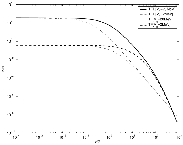
Figure 1: This figure illustrates the differences of the electron density among the different models with different quark chemical potentials. $N=\left(\frac{m_{e}c}{\hbar}\right)^{3}=1.7\times 10^{-8}$fm^-3. $Z=\frac{\hbar}{m_{e}c}=3.9\times 10^{2}$fm. $z$ is the height to the strange quark matter surface. $n$ is the electron number density of $z$. In the extremely relativistic case, the difference between the electron density curves of TF and TFD models is not significant when the density $n$ is very high, but is significant when $n$ is lower. In the high-density domain, TFD-generally-relativistic electron density is about 2 orders of magnitude more than TF-extremely-relativistic electron density, while TFD-electron density is much less than TF-electron density in the low-density domain.

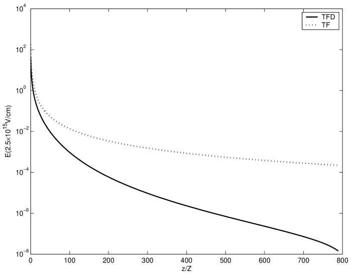
Figure 2: This figure illustrates the differences between the electric fields, $E$, in the TFD model and the TF model. The maximums of the electric field in the two models are both stronger than the critical field $\sim 10^{16}$V/cm. $Z=\frac{\hbar}{m_{e}c}=3.9\times 10^{2}$fm.

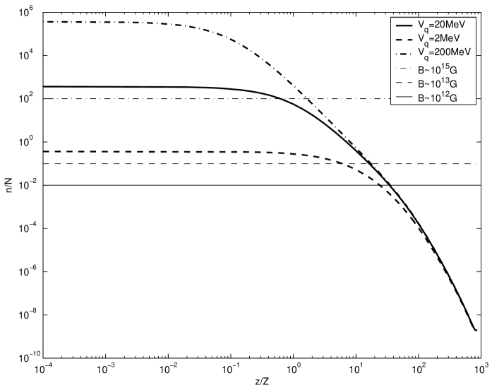
Figure 3: This figure illustrates the differences of the electron density among the different quark chemical potential in the TFD model. $z$ is the height to the strange quark matter surface. $n$ is the electron number density of $z$. In the high-density domain, the electron distributions of different quark chemical potentials are very different. Nevertheless, in the low-density domain, the three electron distributions have few differences. The lowest horizontal line is correspondent to $n^{*}(B=10^{12}$G$)$. The middle horizontal line, which is to $n^{*}(B=10^{13}$G$)$, could tell the difference between $V_{q}=20$ MeV and $V_{q}=2$ MeV. The highest horizontal line, which is to $n^{*}(B=10^{15}$G$)$, may tell the difference between $V_{q}=200$ MeV and $V_{q}=20$ MeV.

References

- (1) Lattimer J M, Prakash M 2004 Science 304 536
- (2) Weber F 2005 Prog. Part. Nucl. Phys. 54 193
- (3) Alcock C, Farhi E and Olinto A 1986 ApJ 310 261
- (4) Haensel P, Zdunik J L, Schaeffer R 1986 A&A 160 121
- (5) Glendenning N K 1996 Compact Stars: Nuclear Physics, Particle Physics, and General Relativity (New York: Springer)
- (6) Cheng K S, Dai Z G, Lu T 1998 Int. J. Mod. Phys. D 7 139
- (7) Weber F 1999 J. Phys. G 25 195
- (8) Cheng K S, Harko T 2000 Phys. Rev. D 62 083001
- (9) Alford M, Reddy S 2003 Phys. Rev. D 67 074024
- (10) Lugones G, Horvath J E 2003 A&A 403 173
- (11) Xu R X 2007 in: the proceedings of Astrophysics of Compact Objects, in press (arXiv:0709.1305)
- (12) Usov V V, Harko T, Cheng K S 2005 ApJ 620 915
- (13) Witten E 1984 Phys. Rev. 30 272
- (14) Xu R X, Qiao G J 1999 Chin. Phys. Lett. 16 778
- (15) Xu R X, Qiao G J 1998 Chin. Phys. Lett. 15 934
- (16) Chen A B, Yu T H, Xu R X, 2007, ApJ, 668 L55
- (17) Xu R X, 2002, ApJ, 570 L65
- (18) Kettner C, Weber F, Weigel M K, Glendenning N K 1995 Phys. Rev. D 51 1440
- (19) Hu J, Xu R X 2002 A&A 387 710
- (20) Schwinger J 1951 Phys. Rev. 82 664
- (21) Usov V V 1998 Phys. Rev. Lett. 80 230
- (22) Usov V V 2001 ApJ 550 L179
- (23) Aksenov A G, Milgrom M, Usov V V 2003 MNRAS 343 L69
- (24) Sanwal D, Pavlov G G, Zavlin V E, Teter M A 2002 ApJ 574 61
- (25) Ruder H, Wunner G, Herold H, Geyer F, 1994 Atoms in Strong Magnetic Fields (Berlin: Springer)
- (26) Mori K, Hailey C J 2002 ApJ 564 914
- (27) Xu R X, Wang H G, Qiao G J 2003 Chin. Phys. Lett. 20 314
- (28) Dreizler R M, Gross E K U, 1990 Density Functional Theory (Springer-Verlag)
- (29) Kohn W, Sham L J 1965 Phys. Rev. 140 A1133
- (30) Jaikumar P 2006 in: Proceedings the IXth Workshop on High Energy Physics Phenomenology, Pramana 67 937-950 (hep-ph/0604179)