FIELD-INDUCED SPIN EXCITATIONS IN RASHBA-DRESSELHAUS TWO-DIMENSIONAL ELECTRON SYSTEMS PROBED BY SURFACE ACOUSTIC WAVES

Abstract

A spin-rotation symmetry in spin-orbit coupled two-dimensional electron systems gives rise to a long-lived spin excitation that is robust against short-range impurity scattering. The influence of a constant in-plane electric field on this persistent spin helix is studied. To probe the field-induced eigen-modes of the spin-charge coupled system, a surface acoustic wave is exploited that provides the wave-vector for resonant excitation. The approach takes advantage of methods worked out in the field of space-charge waves. Sharp resonances in the field dependence of the in-plane and out-of-plane magnetization are identified.

I Introduction

The perspectives of exploiting electron spin for information processing in spintronic devices stimulated basic research of spin-related phenomena.RMP_323 In order to take advantage of traditional semiconductor technologies, the exclusive application of electric fields to generate and manipulate a nonequilibrium spin density is of particular interest. In this respect, the spin-orbit interaction (SOI) provides an attractive mechanism for the pure electric manipulation of moving spins in nonmagnetic semiconductors. Unfortunately, the very same SOI depends on the carrier momentum, which is randomized by elastic and inelastic scattering. This momentum dependence of the coupling leads to the dominant spin relaxation and dephasing in III-V semiconductors known as Dyakonov-Perel relaxation mechanism.Dyakonov In general, however, details of spin dephasing depend on the involved scattering mechanisms, the band structure, and the crystal orientation (see Ref. JAP_073702 and references therein).

An sizable anisotropy of the spin relaxation has been theoretically predicted PRB_15582 ; JPC_R271 for semiconductor heterostructures grown along the [001] axis. According to these studies, a large spin-relaxation anisotropy should exist for the in-plane spin polarization. Moreover, under the condition that the strengths of Rashba ($\alpha$) and Dresselhaus ($\beta$) spin-orbit coupling constants become equal ($\alpha=\beta$), the anisotropy should be maximal. Based on this observation a proposal for a novel spin-transistor device PRL_146801 was put forward. Recent experimental data provided strong evidence for a huge in-plane anisotropy of the spin dephasing time in [001] GaAs/Al_xGa_1-xAs quantum wells.PRB_033305 ; APL_112111 ; PRB_073309 The efficient suppression of relaxation for spins aligned along the [110] orientation in heterostructures with equal Rashba and Dresselhaus SOI strengths is an important result that certainly stimulates further progress in spintronics.

Other promising structures for spintronic applications are quantum well samples grown along the [110] direction. Very long spin-relaxation times on the order of nanoseconds were experimentally demonstrated for the out-of plane spin polarization in such heterostructures.PRL_4196 ; PRL_036603 This effect is caused by the absence of Dyakonov-Perel spin relaxation in the particular crystal direction.

The common physical origin for weak spin relaxation in [110] quantum wells as well as in [001] heterostructures with $\alpha=\beta$ is the presence of an spin-rotation symmetry in the two-dimensional electron gas (2DEG).PRL_236601 This symmetry is robust and leads to an infinite spin lifetime and a persistent spin helix for an idealized model. The theoretical explanation, which has recently been confirmed by experiment,PRL_076604W will initiate a number of further studies in this field. It is the aim of this paper to contribute to this development by treating weakly damped eigen-excitations of the coupled spin-charge system subject to a constant electric field. Our approach bears some similarities with a traditional field in solid state physics namely the study of space-charge waves in crystals.BuchPetrov1 The electric-field-mediated excitations of the coupled spin-charge system are probed by a simulated experimental set up, which provides the wave vector to resonantly excite internal eigen-modes of the biased SOI coupled 2DEG. We focus on excitation mechanisms that exploit surface acoustic waves.

II Basic Theory

Our model is based on a Hamiltonian that describes conduction band electrons in a III-V semiconductor quantum well grown in the [001] direction, which is used to be the $z$ axis of the coordinate system

$$H_{0}=\frac{\hbar^{2}\bm{k}^{2}}{2m}+\hbar\bm{\omega}_{\bm{k}}\cdot\bm{\sigma}.$$ (1)

The effective electron mass, the in-plane wave vector, and the Pauli matrices are denoted by $m$, $\bm{k}$, and $\sigma_{i}$ ($i=x,y,z$), respectively. The precession frequencies $\bm{\omega}_{\bm{k}}$ are due to the SOI, which contain both linear Rashba and Dresselhaus contributions

$$\bm{\omega}_{\bm{k}}^{R}=\frac{\alpha}{\hbar}(k_{y},-k_{x}),\quad\bm{\omega}_{\bm{k}}^{D}=\frac{\beta}{\hbar}(k_{x},-k_{y}),$$ (2)

with $\alpha$, $\beta$ being the respective spin-orbit coupling constants. These vectors are also interpreted as a momentum-dependent internal magnetic field that acts on the carrier motion. The neglected cubic terms to the frequency vector $\bm{\omega}_{\bm{k}}$ play only a secondary role in our study. Throughout this work, it is assumed that the spin-orbit coupling energy is much smaller than the Fermi energy $\varepsilon_{F}$. The model is complemented by the inclusion of elastic scattering on a short-range impurity potential characterized by the elastic scattering time $\tau$.

To elucidate the peculiarities of the spin-orbit coupled 2DEG, the coordinate system is rotated so that the [110] direction becomes a coordinate axis ($k_{\pm}=(k_{x}\pm k_{y})/\sqrt{2}\rightarrow r_{\pm}=(r_{x}\pm r_{y})/\sqrt{2}$). Along the spatial $r_{+}$ axis, a constant electric field $E_{0}$ is applied. In addition, a surface acoustic wave (SAW) with the wave number $K_{SAW}$ and frequency $\Omega=v_{SAW}K_{SAW}$ ($v_{SAW}$ is the sound velocity) should propagate in the same direction giving rise to an internal electric field. The total electric field $E_{+}$ is expressed by

$$E_{+}(r_{+},t)=E_{0}+E_{SAW}\cos(K_{SAW}r_{+}-\Omega t)+\delta E(r_{+},t),$$ (3)

is self-consistently calculated by taking into account the Poisson equation

$$\frac{\partial\delta E(r_{+},t)}{\partial r_{+}}=\frac{4\pi e}{\varepsilon}(F-n),$$ (4)

with $F$ and $n$ denoting the nonequilibrium and initially homogeneous carrier density, respectively (the components of the spin-density matrix $F_{\mu}$, ($\mu=1,2,3,4$) are defined as in Ref. PRB_205326 ). $\varepsilon$ is the dielectric constant. Due to the excitation conditions in Eqs. (3) and (4), all quantities are independent of the spatial coordinate $r_{-}$ for an infinite 2DEG. Along the $r_{+}$ axis, periodic boundary conditions are assumed.

All electric field components act both on the charge and spin degrees of freedom leading to specific field-induced eigen-modes of the spin-charge-coupled system. The appearance and excitation of these modes is treated by drift-diffusion equations that are obtained from a kinetic theory for the spin-density matrix. For the given orientation of the constant electric field $E_{0}$ and the SAW field, the set of equations decouples and takes the form PRB_205326

$$\left[\frac{\partial}{\partial t}-D\frac{\partial^{2}}{\partial r_{+}^{2}}\right]F+\mu\frac{\partial E_{+}F}{\partial r_{+}}-\frac{\hbar}{2m}K_{+}\frac{\partial F_{-}}{\partial r_{+}}=0,$$ (5)

$$\left[\frac{\partial}{\partial t}-D\frac{\partial^{2}}{\partial r_{+}^{2}}+\frac{2}{\tau_{s-}}\right]F_{-}+\mu\frac{\partial E_{+}F_{-}}{\partial r_{+}}-\frac{2}{\tau_{s-}}\frac{F_{-}^{(0)}}{nE_{0}}\left[E_{+}-\frac{2D}{\mu}\frac{\partial}{\partial r_{+}}\right]F=0,$$ (6)

$$\left[\frac{\partial}{\partial t}-D\frac{\partial^{2}}{\partial r_{+}^{2}}+\frac{2}{\tau_{s+}}\right]F_{+}+\mu\frac{\partial E_{+}F_{+}}{\partial r_{+}}-K_{+}\left(\mu E_{+}-2D\frac{\partial}{\partial r_{+}}\right)F_{z}=0,$$ (7)

$$\left[\frac{\partial}{\partial t}-D\frac{\partial^{2}}{\partial r_{+}^{2}}+\frac{2}{\tau_{s}}\right]F_{z}+\mu\frac{\partial E_{+}F_{z}}{\partial r_{+}}+K_{+}\left(\mu E_{+}-2D\frac{\partial}{\partial r_{+}}\right)F_{+}=G_{z},$$ (8)

where $F_{\pm}$ and $F_{z}$ denote the in-plane and out-of plane nonequilibrium spin densities, respectively. $D$ is the diffusion coefficient, $\mu$ the carrier mobility, and $K_{+}=2m(\alpha+\beta)/\hbar^{2}$ a wave number constructed from the spin-orbit coupling constants. In addition, we introduced the spin-relaxation times

$$\frac{1}{\tau_{s}}=4DK^{2},\quad\frac{1}{\tau_{s+}}=\frac{\cos^{2}\varphi}{\tau_{s}},\quad\frac{1}{\tau_{s-}}=\frac{\sin^{2}\varphi}{\tau_{s}},$$ (9)

with $K=m\sqrt{\alpha^{2}+\beta^{2}}/\hbar^{2}$. The angle $\varphi$ is used to quantify the coupling constants according to $\alpha/\sqrt{\alpha^{2}+\beta^{2}}=\cos(\varphi+\pi/4)$ and $\beta/\sqrt{\alpha^{2}+\beta^{2}}=\sin(\varphi+\pi/4)$. For the limiting cases of a pure Rashba and Dresselhaus model, we have $\varphi=-\pi/4$ and $\pi/4$, respectively. When the SAW field is switched off, the applied constant electric field $E_{0}$ induces a homogeneous in-plane magnetization $F_{-}^{(0)}$ that is calculated from

$$F_{-}^{(0)}=\sqrt{2}\frac{\cos^{2}\varphi}{\sin\varphi}\hbar K\mu E_{0}\frac{dn}{d\varepsilon_{F}}.$$ (10)

Taking into account the Einstein relation $\mu=eDd\ln n/d\varepsilon_{F}$, this magnetization is expressed by the result $F_{-}^{(0)}=\hbar K\mu E_{0}dn/d\varepsilon_{F}$ (with $K=m\alpha/\hbar^{2}$) for a Rashba model ($\beta=0$) that was derived by Edelstein. Edelstein When the SOI coupling strengths become equal ($\alpha=\beta$), the spin-relaxation time $\tau_{s-}$ diverges so that the result for $F_{-}^{(0)}$ strongly depends on the initial condition and/or additional spin relaxation mechanisms quantified by the scattering time $\tau_{sp}$ ($\tau_{s-}^{-1}\rightarrow\tau_{s-}^{-1}+\tau_{sp}^{-1}$). The divergency is also circumvented in the ac response.PRB_205326 ; IJMPB_4937 In all cases, the field-induced in-plane magnetization disappears for $\alpha=\beta$. In Eq. (8), $G_{z}$ describes the uniform generation of an out-of plane spin polarization by optical means or by the application of a perpendicular constant magnetic field.

From Eqs. (4) and (5), an expression for the total time-dependent charge current density $I(t)$ is obtained

$$j(r_{+},t)+\frac{\varepsilon}{4\pi}\frac{\partial\delta E}{\partial t}=I(t),\quad j(r_{+},t)=e\mu E_{+}F-eD\frac{\partial F}{\partial r_{+}}-\sqrt{2}\frac{\hbar K}{m}\cos\varphi eF_{-},$$ (11)

which completes the set of basic equations necessary to study electric-field-mediated effects in the spin-charge coupled 2DEG. The drift-diffusion Eqs. (5) to (8) decouple into two sets of equations for the components $F$, $F_{-}$ and $F_{z}$, $F_{+}$. Accordingly, the spin-charge coupling prescribed by Eqs. (5) and (6) is treated in the next Section, whereas Eqs. (7) and (8) are solved in Section 4.

III Spin-charge coupling

The solution of Eqs. (5) to (8) is facilitated by the fact that all quantities depend only on $z=K_{SAW}r_{+}-\Omega t$. The derivative with respect to $z$ is denoted by a prime. Introducing the dimensionless functions $f=F/n$, $f_{\pm}=F_{\pm}/n$, and $f_{z}=F_{z}/n$ and the parameters

$$Y_{+}=\frac{E_{+}}{E_{0}},\quad Y=\frac{\delta E}{E_{0}},\quad\Omega_{E}=\mu E_{0}K_{SAW},\quad\frac{1}{\tau_{M}}=\frac{4\pi e}{\varepsilon}\mu n,\quad\Lambda=\frac{DK_{SAW}}{\mu E_{0}},$$ (12)

we obtain the following set of coupled ordinary differential equations

$$-\Omega f_{-}^{\prime}-\Lambda\Omega_{E}f_{-}^{\prime\prime}+\frac{2}{\tau_{s-}}f_{-}+\Omega_{E}\left(Y_{+}f_{-}\right)^{\prime}+\frac{2}{\tau_{s-}}f_{-}^{(0)}\left(Y_{+}f-2\Lambda f^{\prime}\right)=0,$$ (13)

$$-\Omega\tau_{M}Y^{\prime}+Y_{+}f-\Lambda f^{\prime}-\sqrt{2}\frac{\hbar K}{m\mu E_{0}}\cos\varphi f_{-}=\frac{I}{j_{0}},\quad\Omega_{E}\tau_{M}Y^{\prime}=f-1.$$ (14)

These equations are solved by applying perturbation theory with respect to the SAW electric field $E_{SAW}$. When the SAW field is absent ($E_{SAW}=0$), all quantities are independent of $z$ and we obtain for the constant charge current density

$$I_{0}=j_{0}\left(1-\sqrt{2}\frac{\hbar K}{m\mu E_{0}}\cos\varphi f_{-}^{(0)}\right),$$ (15)

with $j_{0}=en\mu E_{0}$. The spin-induced contribution on the right-hand side of this equation results from the homogeneous in-plane magnetization $f_{-}^{(0)}$ that vanishes for a system with equal Rashba and Dresselhaus coupling constants ($\alpha=\beta$).

To proceed, we calculate the stationary current contribution $\delta I$ associated with the SAW electric field. This time-independent current contribution arises from carriers that are driven by the SAW. A similar current can also be generated by a moving optical lattice in a photorefractive crystal. As a periodic boundary condition along the $r_{+}$ axis is assumed, the solution is searched for in the form of a Fourier series $f(z)=n+\delta f(z)$, $\delta f(z)=\sum_{p}\exp(ipz)\delta f(p)$. Taking into account the Fourier transformed version of Eq.(11)

$$\frac{I}{j_{0}}\delta_{p,0}=-ip\Omega\tau_{M}Y(p)+\sum\limits_{p^{\prime}}Y_{+}(p-p^{\prime})f(p^{\prime})-ip\Lambda f(p)-\sqrt{2}\frac{\hbar K}{m\mu E_{0}}\cos\varphi f_{-}(p),$$ (16)

we obtain

$$\frac{\delta I}{j_{0}}=\frac{Y_{SAW}}{2}\left[1-\sqrt{2}\frac{\hbar K}{m\mu E_{0}}\cos\varphi f_{-}^{(0)}\right]\left[\delta f(1)+\delta f(-1)\right],$$ (17)

with $Y_{SAW}=E_{SAW}/E_{0}$. The nonequilibrium fluctuation of the charge density $\delta f(1)$ for $p=1$ is expressed by the variation of the internal electric field $\delta Y(1)$ via $\delta Y(1)=-i\delta f(1)/(\Omega_{E}\tau_{M})$. The latter quantity is calculated from the Fourier transformed Eqs. (13) and (14), which are given by

$$\left[-ip(\Omega-\Omega_{E}+ip\Lambda\Omega_{E})+\frac{2}{\tau_{s-}}\right]\delta f_{-}(p)$$ (18)

$$+f_{-}^{(0)}\left[ip\Omega_{E}+\frac{2}{\tau_{s-}}\left(1+ip\Omega_{E}\tau_{M}\right)\right]\delta Y(p)+4p^{2}\frac{\Lambda}{\tau_{s-}}f_{-}^{(0)}\delta Y(p)$$

$$=-\frac{1}{\tau_{s-}}f_{-}^{(0)}Y_{SAW}(\delta_{p,1}+\delta_{p,-1})-\frac{i\Omega_{E}}{2}f_{-}^{(0)}Y_{SAW}(\delta_{p,1}-\delta_{p,-1}),$$

$$\left[1-ip\tau_{M}(\Omega-\Omega_{E}(1-ip\Lambda))\right]\delta Y(p)-\sqrt{2}\frac{\hbar K}{m\mu E_{0}}\cos\varphi\delta f_{-}(p)$$

$$=-\frac{1}{2}Y_{SAW}(\delta_{p,1}+\delta_{p,-1}).$$ (19)

Even at the absence of SOI, the SAW field alone gives rise to a charge current that is easily calculated from Eqs. (18), (19), and (17)

$$\left(\frac{\delta I}{j_{0}}\right)_{1}=\frac{Y_{SAW}^{2}\Omega_{E}}{2}\frac{\Omega-\Omega_{E}}{(\Omega-\Omega_{E})^{2}+(\tau_{M}^{-1}+DK_{SAW}^{2})^{2}}.$$ (20)

This current contribution is due to space-charge waves, the dispersion relation of which is obtained from the poles in Eq. (20)

$$\Omega=\mu E_{0}K_{SAW}-i\left(\frac{1}{\tau_{M}}+DK_{SAW}^{2}\right),$$ (21)

where $\tau_{M}$ denotes the Maxwellian relaxation time. The physical origin of this mode, which has been thoroughly studied in the field of photorefractive materials BuchPetrov1 , are oscillations of the free electron gas. In the same way as the current density $j_{0}$ has a spin complement in Eq. (15), the well-known SAW-induced charge current in Eq. (20) has a related spin contribution, which is also calculated from Eqs. (17) and (18), (19) with the result

$$\left(\frac{\delta I}{j_{0}}\right)_{2}=\frac{\hbar}{4m}\frac{K_{+}K_{SAW}f_{-}^{(0)}Y_{SAW}^{2}}{\left[(\Omega-\Omega_{E})^{2}+\left(\tau_{M}^{-1}+DK_{SAW}^{2}\right)^{2}\right]\left[\left(\Omega-\Omega_{E}\right)^{2}+\left(2/\tau_{s-}+DK_{SAW}^{2}\right)^{2}\right]}$$

$$\times\Biggl{\{}(\Omega-\Omega_{E})\left(\frac{2}{\tau_{s-}}+DK_{SAW}^{2}\right)\left(\frac{2}{\tau_{s-}}-\frac{1}{\tau_{M}}\right)$$ (22)

$$+\Omega\left[\left(\frac{1}{\tau_{M}}+DK_{SAW}^{2}\right)\left(\frac{2}{\tau_{s-}}+DK_{SAW}^{2}\right)-\left(\Omega-\Omega_{E}\right)^{2}\right]\Biggl{\}}.$$

The SAW-induced electronic current in Eq. (20) is independent of the spin-degree of freedom and disappears at the resonance frequency $\Omega=\Omega_{E}$ of space-charge waves. This result has to be compared with Eq. (22) that holds for the spin complement of the SAW-induced charge current, which may exhibit a sharp resonance at $\Omega=\Omega_{E}$. Besides space-charge excitations that also appear in Eq. (20), there exists a new eigen-mode, in which $\tau_{M}^{-1}$ is replaced by the spin-scattering rate $2/\tau_{s-}$ that vanishes for $\alpha=\beta$. This spin-mediated mode has the character of a space-charge wave with an infinite Maxwellian relaxation time (for $\alpha=\beta$). In experiment, the SAW related stationary charge currents in Eqs. (20) and (22) can be distinguished by their qualitative different dependence on the electric field $E_{0}$.

IV Spin-spin coupling

For the considered set-up not all four components of the spin-density matrix couple to each other. According to the special field orientation, the coupling between the spin components $F_{z}$ and $F_{+}$ is separated from the charge density $F$ and the in-plane spin component $F_{-}$. The related drift-diffusion Eqs. (7) and (8) take the dimensionless form

$$-\Omega f_{+}^{\prime}-\Lambda\Omega_{E}f_{+}^{\prime\prime}+\frac{2}{\tau_{s+}}f_{+}+\Omega_{E}(Y_{+}f_{+})^{\prime}-\frac{K_{+}\Omega_{E}}{K_{SAW}}Y_{+}f_{z}+2\frac{K_{+}\Omega_{E}\Lambda}{K_{SAW}}f_{z}^{\prime}=0,$$ (23)

$$-\Omega f_{z}^{\prime}-\Lambda\Omega_{E}f_{z}^{\prime\prime}+\frac{2}{\tau_{s}}f_{z}+\Omega_{E}(Y_{+}f_{z})^{\prime}+\frac{K_{+}\Omega_{E}}{K_{SAW}}Y_{+}f_{+}-2\frac{K_{+}\Omega_{E}\Lambda}{K_{SAW}}f_{+}^{\prime}=\frac{G_{z}}{n},$$ (24)

where $G_{z}$ denotes the source of an out-of-plane spin polarization. Without the application of the SAW field, we obtain the steady-state solution

$$f_{z}^{(0)}=\frac{G_{z}/n}{2/\tau_{s}+(\mu E_{0})^{2}/D},\quad f_{+}^{(0)}=-\frac{\mu E_{0}}{DK_{+}}f_{z}^{(0)}.$$ (25)

The out-of-plane spin polarization $f_{z}^{(0)}$ is suppressed by the electric field.Kalevich By determining this suppression in experiment, the spin-relaxation time $\tau_{s}$ can be determined in a way similar to the well established experimental set up that is based on the Hanle effect (c.f., for instance, Ref. PRB_033305 ). Furthermore, the electric field $E_{0}$ induces an in-plane spin polarization $f_{+}^{(0)}$.

As in Section 3, the effect of the SAW is treated by a perturbation expansion $f_{z}=f_{z}^{(0)}+\delta f_{z}$ and $f_{+}=f_{+}^{(0)}+\delta f_{+}$. The Fourier transformed basic Eqs. (23) and (24) are easily solved, when non-linear perturbations are neglected. The solution for the lowest-order Fourier components is given in the Appendix.

To determine the steady-state spin polarization under the mutual influence of a constant electric field and the SAW field, we focus on the most interesting case $\alpha=\beta$ and assume $\Omega_{E}\tau_{M}\gg 1$. Under these conditions, the solution given by Eqs. (31) to (33) simplifies and takes the form

$$\frac{\delta f_{+}(0)}{f_{+}^{(0)}}=-\frac{Y_{SAW}^{2}\Omega_{E}}{2(1+\Lambda_{+}^{2})}{\rm Re}\Biggl{\{}\frac{\Omega_{E}(1-q^{2})Z_{1}+\Omega(1-\Lambda_{+}^{2}-2iq\Lambda_{+})}{(\Omega-\Omega_{+})(\Omega-\Omega_{-})}\Biggl{\}},$$ (26)

$$\frac{\delta f_{z}(0)}{f_{z}^{(0)}}=\frac{Y_{SAW}^{2}\Omega_{E}}{2\Lambda(1+\Lambda_{+}^{2})}{\rm Re}\Biggl{\{}\frac{\Omega_{E}(1-q^{2})Z_{2}+i\Omega(1-\Lambda_{+}^{2}+2iq\Lambda)}{(\Omega-\Omega_{+})(\Omega-\Omega_{-})}\Biggl{\}},$$ (27)

with the shorthand notations $Z_{1}=3\Lambda_{+}-1+i\Lambda(1-\Lambda_{+}^{2})$, $Z_{2}=\Lambda(3-2i\Lambda+\Lambda_{+}^{2})$, $q=K_{+}/K_{SAW}$, and $\Lambda_{+}=q\Lambda$. The eigen-frequencies of the spin excitations are expressed by

$$\Omega_{\pm}=\mu E_{0}(K_{SAW}\pm K_{+})-iD(K_{SAW}\pm K_{+})^{2}.$$ (28)

The appearance of resonances at $\Omega=\Omega_{\pm}$ that occur in the in-plane and out-of-plane field-induced spin polarization is the most remarkable result of this paper. Due to the spin-rotation symmetry, a soft mode develops in the system that can be probed by a SAW, which provides the wave vector $K_{SAW}$ for the resonant excitation. The low-frequency mode $\Omega\rightarrow 0$ becomes increasingly undamped for $K_{SAW}\rightarrow\pm K_{\pm}$. As a remnant of these coherent long-lived spin excitations, a weakly damped resonance appears, when the applied constant electric field $E_{0}$ satisfies the condition $\Omega=v_{SAW}K_{SAW}=\mu E_{0}(K_{SAW}-K_{+})$.

Numerical examples are shown in Figs. 2 and 2 for the SAW-induced

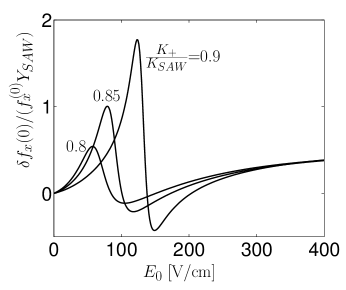
Figure 1: SAW-induced stationary in-plane spin polarization $\delta f_{x}(0)$ referred to $f_{x}^{(0)}Y_{SAW}$ for $\lambda_{SAW}=5.6$ $\mu$m, $\mu=2.3\,10^{4}$ cm²/Vs, and $D=24$ cm²/s. Results are shown for $K_{+}/K_{SAW}=$ 0.8, 0.85, and 0.9.

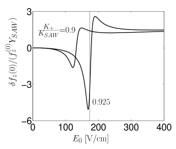
Figure 2: SAW-induced stationary out-of-plane spin polarization $\delta f_{z}(0)$ referred to $f_{z}^{(0)}Y_{SAW}$ for $\lambda_{SAW}=5.6$ $\mu$m, $\mu=2.3\,10^{4}$ cm²/Vs, and $D=24$ cm²/s. Results are shown for $K_{+}/K_{SAW}=$ 0.9 and 0.925.

in-plane and out-of-plane spin polarization. The parameters used in the calculation refer to GaAs quantum wells.PRL_036603 ; PRL_047602 It is to be noted that in the displayed relative spin polarizations, the electric field $E_{0}$ enters via the field-dependent quantities $f_{x}^{(0)}$ and $f_{z}^{(0)}$ calculated from Eq. (25). Both components of the magnetization exhibit a sharp resonance in the electric field dependence at $\mu E_{0}=v_{SAW}/(1-K_{+}/K_{SAW})$ as indicated by the vertical line in Fig. 2. With increasing ratio $K_{+}/K_{SAW}$, the resonance is shifted to higher field strengths and becomes more pronounced. Under the condition $E_{SAW}\approx E_{0}$ and at the resonance, the out-of-plane spin polarization may significantly exceed the spin generation $f_{z}^{(0)}$ given in Eq. (25). As the suppression of $f_{z}^{(0)}$ at high electric fields can be compensated by an appropriate in-plane magnetic field PRB_075340 , the experimental demonstration of the effect should be feasible. Its most salient feature is the strong variation of the field-induced magnetization in the vicinity of the resonance field strength. This switching of the magnetization caused by an applied constant electric field could be useful for future spintronic device applications.

V Summary

Recently, long-range transport of spins has been experimentally demonstrated in [001] GaAs quantum wells with balanced Rashba and Dresselhaus terms as well as in Dresselhaus [110] quantum wells. The idealized model that describes both systems exhibits an exact spin rotation symmetry with an associated soft mode and a persistent spin helix. This long-lived spin coherence state is transferred to a field-dependent eigenmode of the system, when a constant in-plane electric field is applied. To resonantly probe the field-induced excitation, the required wave-vector must be provided by an appropriate experimental set up. Similar to the well established physics of space-charge waves one can produce optical gratings for that purpose. In this paper, we treated an excitation mechanism via an acoustic wave propagating along a [001] GaAs quantum well, in which both Rashba and Dresselhaus SOI exist. Due to the spin-charge coupling, specific eigenmodes are identified both in the charge current density and the in-plane and out-of-plane spin polarizations. The SAW-induced change of the stationary charge current is composed of two contributions. The first one is independent of the SOI and exhibits a pole that is due to oscillations of the free carrier density. In the second contribution, which is related to the field-induced homogeneous spin accumulation, a new eigenmode appears with the dispersion relation $\Omega=\mu E_{0}K_{SAW}-(DK_{SAW}^{2}+2/\tau_{s-})$. In this equation, the spin-scattering time $\tau_{s-}$ (which diverges in the case $\alpha=\beta$) takes over the role of the Maxwellian relaxation time $\tau_{M}$ that is responsible for the damping of pure charge oscillations.

Characteristic field-dependent eigenmodes appear also in the SAW-induced components of the magnetization. Most interesting is the case, when the Rashba and Dresselhaus coupling strengths become equal. According to the dispersion relation $\Omega=\Omega_{-}$, a undamped soft mode occurs, when the wave-vector $K_{SAW}$ of the SAW approaches the shifting vector $K_{+}=2m(\alpha+\beta)/\hbar^{2}$. As a remnant of this persistent spin helix, a sharp resonance occurs in the electric-field dependence of the in-plane and out-of-plane magnetization at $\mu E_{0}=v_{SAW}/(1-K_{+}/K_{SAW})$. In the vicinity of this resonance, the spin polarization drastically changes with a slight variation of the electric field strength. It is a challenge to experimentally verify this field-induced switching of magnetization in a 2DEG with balanced Rashba and Dresselhaus SOI.

Solution of kinetic equations In this Section, the coupled Eqs. (23) and (24) are solved by a perturbation approach with respect to the SAW electric field $Y_{SAW}$. First, the equations are expressed in terms of a Fourier series, which leads to the result

$$\left[-ip\Omega+p^{2}\Lambda\Omega_{E}+\frac{2}{\tau_{s+}}+ip\Omega_{E}\right]\delta f_{+}(p)+\frac{ipY_{SAW}\Omega_{E}}{2}\left[\delta f_{+}(p+1)+\delta f_{+}(p-1)\right]$$

$$-\frac{K_{+}\Omega_{E}}{K_{SAW}}(1-2ip\Lambda)\delta f_{z}(p)-\frac{K_{+}Y_{SAW}\Omega_{E}}{2K_{SAW}}\left[\delta f_{z}(p+1)+\delta f_{z}(p-1)\right]$$ (29)

$$=f_{+}^{0}\Omega_{E}\left[\frac{Y_{SAW}}{2i}(\delta_{p,1}-\delta_{p,-1})-ipY(p)\right]+\frac{K_{+}f_{z}^{0}\Omega_{E}}{K_{SAW}}\left[\frac{Y_{SAW}}{2}(\delta_{p,1}+\delta_{p,-1})+Y(p)\right],$$

$$\left[-ip\Omega+p^{2}\Lambda\Omega_{E}+\frac{2}{\tau_{s}}+ip\Omega_{E}\right]\delta f_{z}(p)+\frac{ipY_{SAW}\Omega_{E}}{2}\left[\delta f_{z}(p+1)+\delta f_{z}(p-1)\right]$$

$$+\frac{K_{+}\Omega_{E}}{K_{SAW}}(1-2ip\Lambda)\delta f_{+}(p)+\frac{K_{+}Y_{SAW}\Omega_{E}}{2K_{SAW}}\left[\delta f_{+}(p+1)+\delta f_{+}(p-1)\right]$$ (30)

$$=f_{+}^{0}\Omega_{E}\left[\frac{Y_{SAW}}{2i}(\delta_{p,1}-\delta_{p,-1})-ipY(p)\right]-\frac{K_{+}f_{+}^{0}\Omega_{E}}{K_{SAW}}\left[\frac{Y_{SAW}}{2}(\delta_{p,1}+\delta_{p,-1})-Y(p)\right].$$

To calculate the steady-state solution, the equations for the $p=0$ components $\delta f_{+}(0)$ and $\delta f_{z}(0)$ are solved. We obtain

$$\delta f_{+}(0)=\frac{Y_{SAW}}{1+2(\alpha^{2}+\beta^{2})\Lambda_{+}^{2}/(\alpha+\beta)^{2}}{\rm Re}\left[\Lambda_{+}\delta f_{z}(1)-\delta f_{+}(1)\right],$$ (31)

$$\delta f_{z}(0)=-\frac{Y_{SAW}}{1+2(\alpha^{2}+\beta^{2})\Lambda_{+}^{2}/(\alpha+\beta)^{2}}{\rm Re}\left[\Lambda_{+}\delta f_{+}(1)+\delta f_{z}(1)\right].$$ (32)

In a second step, the Fourier components $\delta f_{+}(1)$ and $\delta f_{z}(1)$ have to be calculated. Disregarding nonlinear contributions, the remaining equations are easily solved with the result

$$\delta f_{+}(1)=\frac{c_{1}A_{s}-c_{2}B}{A_{s}A_{s+}+B^{2}},\quad\delta f_{z}(1)=-\frac{c_{2}A_{s+}+c_{1}B}{A_{s}A_{s+}+B^{2}},$$ (33)

$$c_{1}=\left(Y(1)+\frac{Y_{SAW}}{2}\right)\left(-if_{+}^{0}+\frac{K_{+}f_{+}^{0}}{K_{SAW}}\right),\quad c_{2}=\left(Y(1)+\frac{Y_{SAW}}{2}\right)\left(if_{z}^{0}+\frac{K_{+}f_{+}^{0}}{K_{SAW}}\right),$$

$$A_{s}=\frac{2}{\Omega_{E}\tau_{s}}+i(1-i\Lambda-\frac{\Omega}{\Omega_{E}}),\quad A_{s+}=\frac{2}{\Omega_{E}\tau_{s+}}+i(1-i\Lambda-\frac{\Omega}{\Omega_{E}}),\quad B=\frac{K_{+}}{K_{SAW}}(1-2i\Lambda).$$

The SAW-induced stationary magnetization of the biased 2DEG is expressed by Eqs. (31) to (33).

References

References

• (1) I. Zutic, J. Fabian, and S. D. Sarma, Rev. Mod. Phys. 76, 323 (2004).
• (2) M. I. Dyakonov and V. I. Perel, JETP Lett. 13, 467 (1971), [Sov. Phys. JETP 33, 1053 (1971)].
• (3) J. L. Cheng and M. W. Wu, J. Appl. Phys. 101, 073702 (2007).
• (4) N. S. Averkiev and L. E. Golub, Phys. Rev. B 60, 15582 (1999).
• (5) N. S. Averkiev, L. E. Golub, and M. Willander, J. Phys.: Condens. Matter 14, R271 (2002).
• (6) J. Schliemann, J. C. Egues, and D. Loss, Phys. Rev. Lett. 90, 146801 (2003).
• (7) N. S. Averkiev, L. E. Golub, A. S. Gurevich, V. P. Evtikhiev, V. P. Kochereshko, A. V. Platonov, A. S. Shkolnik, and Y. P. Efimov, Phys. Rev. B 74, 033305 (2006).
• (8) B. Liu, H. Zhao, J. Wang, L. Liu, W. Wang, D. Chena, and H. Zhu, Appl. Phys. Lett. 90, 112111 (2007).
• (9) D. Stich, J. H. Jiang, T. Korn, R. Schulz, D. Schuh, W. Wegscheider, M. W. Wu, and C. Schüller, Phys. Rev. B 76, 073309 (2007).
• (10) Y. Ohno, R. Terauchi, T. Adachi, F. Matsukura, and H. Ohno, Phys. Rev. Lett. 83, 4196 (1999).
• (11) O. D. D. Couto, F. Iikawa, J. Rudolph, R. Hey, and P. V. Santos, Phys. Rev. Lett. 98, 036603 (2007).
• (12) B. A. Bernevig, J. Orenstein, and S. C. Zhang, Phys. Rev. Lett. 97, 236601 (2006).
• (13) C. P. Weber, J. Orenstein, B. A. Bernevig, S. C. Zhang, J. Stephens, and D. D. Awschalom, Phys. Rev. Lett. 98, 076604 (2007).
• (14) M. P. Petrov and V. V. Bryksin, Photorefractive Materials and their Applications, Eds. P. Guenter and J. P. Huigard (Springer Verlag, Berlin, 2007).
• (15) P. Kleinert and V. V. Bryksin, Phys. Rev. B 76, 205326 (2007).
• (16) V. M. Edelstein, Solid State Commun. 73, 233 (1990).
• (17) V. V. Bryksin and P. Kleinert, Int. J. Mod. Phys. B 20, 4937 (2006).
• (18) V. K. Kalevich and V. L. Korenev, Pis’ma Zh. Eksp. Teor. Fiz. 52, 859 (1990), [JETP Lett. 52, 230 (1990)].
• (19) J. Rudolph, R. Hey, and P. V. Santos, Phys. Rev. Lett. 99, 047602 (2007).
• (20) V. V. Bryksin and P. Kleinert, Phys. Rev. B 76, 075340 (2007).