The Possible Textures in the Seesaw Realization of the Strong Scaling Ansatz and the Implications for Thermal Leptogenesis

Abstract

We classify the textures of the Dirac and the right-handed Majorana neutrino mass matrices, $M_{D}$ and $M_{R}$, which can satisfy the so-called “Strong Scaling Ansatz” (SSA) within the framework of the seesaw mechanism $M_{\nu}=-M_{D}^{T}M_{R}^{-1}M_{D}$. We assume that the Dirac neutrino mass matrix has some texture zeros and examine which elements should be zero in order to satisfy the SSA, by taking into account all possible textures for $M_{R}$. We find that the resulting Dirac neutrino mass matrices have rank 2 as well as the rank of the effective neutrino mass matrix $M_{\nu}$, or rank 1, depending only on the textures of $M_{R}^{-1}$. We also consider the three cases of the breaking of the SSA by introducing a complex breaking parameter in $M_{\nu}$ and show that it can generate the CP violation in the lepton sector as well as non-zero $m_{3}$ and $U_{e3}$. We furthermore discuss the implications of the thermal leptogenesis for the both cases which satisfy and break the SSA in the basis where $M_{R}$ is diagonal.

1 Introduction

Since the discovery of neutrino oscillations by the Super-Kamiokande collaboration, solar, atmospheric, reactor and accelerator neutrino experiments (Super-Kamiokande [1], SNO [2], KamLAND [3], K2K [4] and MINOS [5]) have confirmed the evidence of neutrino oscillations. A global analysis of current experimental data yields [6]

$$0.26\leq \sin^{2}\theta_{12}~{} \leq 0.40\;,$$

$$0.34\leq \sin^{2}\theta_{23} \leq 0.67\;,$$ (1.1)

$$\sin^{2}\theta_{13} \leq 0.050\;,$$

and

$$7.1\times 10^{-5}~{}{\rm eV}^{2}\leq \Delta m_{21}^{2} \leq 8.3\times 10^{-5}~{}{\rm eV}^{2}\;,$$

$$2.0\times 10^{-3}~{}{\rm eV}^{2}\leq |\Delta m_{32}^{2}|~{} \leq 2.8\times 10^{-5}~{}{\rm eV}^{2}\;,$$ (1.2)

at the $3\sigma$.

The structures of neutrino mass matrices have been studied in various models based on both continuous [7] and discrete flavor symmetries [8], and many attempts to connect the flavor symmetry approaches to the grand unified thories have been done [9]. However, these kind of approaches generally receive the corrections from the renormalization group effects. As a new approach independent of the renormalization group effects, R.N. Mohapatra and W. Rodejohann have recently proposed the strong scaling Ansatz (SSA) that the elements of the neutrino mass matrix $(M_{\nu})_{\alpha\beta}\equiv m_{\alpha\beta}$ ($\alpha,\beta=e,\mu,\tau$) satisfy the following scaling

$$\frac{m_{e\mu}}{m_{e\tau}}=\frac{m_{\mu\mu}}{m_{\mu\tau}}=\frac{m_{\tau\mu}}{m_{\tau\tau}}\equiv c\,,$$ (1.3)

in the basis where the charged lepton mass matrix is diagonal, and have shown that such a neutrino mass matrix

$$M_{\nu}=\left(\begin{array}[]{@{\,}ccc@{\,}}A&B&B/c\\ B&D&D/c\\ B/c&D/c&D/c^{2}\end{array}\right)=U{\rm diag}(m_{1},m_{2},m_{3})U^{T}\,,$$ (1.7)

where $U$ is the PMNS matrix, predicts the inverted hierarchy with $m_{3}=0$, vanishing $U_{e3}$ and no CP violation [10], accommodating to the currecnt neutrino experimental data. Here we take the following parameterization for $U$ [12]:

$$U=\left(\begin{array}[]{@{\,}ccc@{\,}}c_{12}c_{13}&s_{12}c_{13}&s_{13}e^{-i\delta}\\ -c_{23}s_{12}-s_{23}s_{13}c_{12}e^{i\delta}&c_{23}c_{12}-s_{23}s_{13}s_{12}e^{i\delta}&s_{23}c_{13}\\ s_{23}s_{12}-c_{23}s_{13}c_{12}e^{i\delta}&-s_{23}c_{12}-c_{23}s_{13}s_{12}e^{i\delta}&c_{23}c_{13}\end{array}\right)P\,,$$ (1.11)

where $s_{ij}\equiv\sin\theta_{ij}$, $c_{ij}\equiv\cos\theta_{ij}$ and $P={\rm diag}(1,e^{i\alpha},e^{i(\beta+\delta)})$ with $\alpha,\beta$ and $\delta$ being the Majorana and Dirac phases. By adjusting the value of the scaling parameter $c$, we can obtain the non-maximal atmospheric neutrino mixing angle which may be favored in future experiments. There are three possible cases of breaking the SSA [10]:

$${\rm A1:}\quad\frac{m_{e\mu}}{m_{e\tau}}=\frac{m_{\mu\mu}}{m_{\mu\tau}}=c\,,\quad\frac{m_{\tau\mu}}{m_{\tau\tau}}=c(1+\epsilon)\,,$$ (1.12)

$${\rm A2:}\quad\frac{m_{e\mu}}{m_{e\tau}}=\frac{m_{\tau\mu}}{m_{\tau\tau}}=c\,,\quad\frac{m_{\mu\mu}}{m_{\mu\tau}}=c(1+\epsilon)\,,$$ (1.13)

$${\rm A3:}\quad\frac{m_{\mu\mu}}{m_{\mu\tau}}=\frac{m_{\tau\mu}}{m_{\tau\tau}}=c\,,\quad\frac{m_{e\mu}}{m_{e\tau}}=c(1+\epsilon)\,,$$ (1.14)

and it has been shown that non-zero $m_{3}$ and $U_{e3}$ can be generated in these three cases [10]. In this paper we will show that both real and complex breaking parameter can generate the CP violation in the lepton sector as well as non-zero $m_{3}$ and $U_{e3}$.

This paper is organized as follows. In section 2, we classify the textures of the Dirac and the right-handed Majorana neutrino mass matrices, $M_{D}$ and $M_{R}$, which can satisfy the SSA within the framework of the seesaw mechanism $M_{\nu}=-M_{D}^{T}M_{R}^{-1}M_{D}$, and show the conditions of elements in $M_{D}$ for getting the SSA by taking into account all possible textures for $M_{R}$. In this section, we also consider the three cases of breaking the SSA by introducing a complex breaking parameter in $M_{\nu}$ and examine which cases of the breaking can be realized within the seesaw framework. In section 3, we briefly review the phenomenology of the SSA and examine the effects of the breaking of the SSA on $m_{3}$, $U_{e3}$ and $J_{{\rm CP}}$ for the three cases A1, A2 and A3, semi-analytically. Numerical analyses for the original case of the SSA and the three cases A1, A2 and A3 will be done in section 4. In section 5, we discuss the implications of the thermal leptogenesis for the both cases which satisfy and break the SSA in the basis where $M_{R}$ is diagonal. Section 6 is devoted to summary.

2 Classification

In this section, we classify the textures of $M_{D}$ and $M_{R}$, which can satisfy the SSA within the framework of the seesaw mechanism $M_{\nu}=-M_{D}^{T}M_{R}^{-1}M_{D}$. In order to do that, we take the form of $M_{D}$ as

$$M_{D}=\left(\begin{array}[]{@{\,}ccc@{\,}}a_{1}&b_{1}&d_{1}\\ a_{2}&b_{2}&d_{2}\\ a_{3}&b_{3}&d_{3}\end{array}\right)\,,$$ (2.4)

and find the conditions of elements in $M_{D}$ for getting the SSA, by taking into account all possible textures for $M_{R}$. First, we mention the most general condition of the elements in $M_{D}$. If $M_{D}$ is taken to be the following form,

$$M_{D}=\left(\begin{array}[]{@{\,}ccc@{\,}}a_{1}&b_{1}&b_{1}/c\\ a_{2}&b_{2}&b_{2}/c\\ a_{3}&b_{3}&b_{3}/c\end{array}\right)\,,$$ (2.8)

then $M_{\nu}$ satisfies the strong scaling, without depending on the textures for $M_{R}$ [13]. Here we assume that $M_{D}$ has some texture zeros and examine which elements should be zero in order to get the SSA. The Dirac neutrino mass matrices with texture zeros are attractive to relate the low energy CP violation in the lepton sector to the high energy CP violation necessary for the thermal leptogeneis [14, 15, 16, 17]. We have listed the conditions of elements in $M_{D}$ for getting the SSA in Tables 1, 2, 3 and 4. It is obvious that the textures of $M_{R}$ for the classes $\tilde{F}_{1}$–$\tilde{F}_{7}$ in Table 3 can be obtained by exchanging the generation indices of those for the classes $F_{1}$–$F_{7}$ in Table 2. Similarly, the classes $G_{2}$ and $G_{3}$ can be obtained from the classes $G_{4}$ and $G_{5}$ in Table 4. From our classification, we have found that the resulting Dirac neutrino mass matrices have rank 2 as well as the rank of the effective neutrino mass matrix $M_{\nu}$, or rank 1, depending only on the textures of $M_{R}^{-1}$; the same texture for $M_{R}^{-1}$ leads to the same conditions for the elements in $M_{D}$.

We also consider the three cases of breaking the SSA by introducing a complex breaking parameter $\epsilon$ in $M_{\nu}$. Here, all parameters are supposed to be complex, and after rephasing, we can redefine $c$, $A$, $B$ and $D$ as real and take the neutrino mass matrices for the three cases A1, A2 and A3 given in Eqs. (1.12), (1.13) and (1.14) as

$${\rm A1:}\quad M_{\nu} = \left(\begin{array}[]{@{\,}ccc@{\,}}A&Be^{i\phi}&Be^{i\phi}/c\\ Be^{i\phi}&D(1+\epsilon)&D(1+\epsilon)/c\\ Be^{i\phi}/c&D(1+\epsilon)/c&D/c^{2}\end{array}\right)\,,$$ (2.12)

$${\rm A2:}\quad M_{\nu} = \left(\begin{array}[]{@{\,}ccc@{\,}}A&Be^{i\phi}&Be^{i\phi}/c\\ Be^{i\phi}&D(1+\epsilon)&D/c\\ Be^{i\phi}/c&D/c&D/c^{2}\end{array}\right)\,,$$ (2.16)

$${\rm A3:}\quad M_{\nu} = \left(\begin{array}[]{@{\,}ccc@{\,}}A&Be^{i\phi}(1+\epsilon)&Be^{i\phi}/c\\ Be^{i\phi}(1+\epsilon)&D&D/c\\ Be^{i\phi}/c&D/c&D/c^{2}\end{array}\right)\,,$$ (2.20)

where $\epsilon\equiv|\epsilon|e^{i\varphi}$ and $|\epsilon|\ll 1$. The conditions of elements in $M_{D}$ for breaking the SSA have also been listed in Tables 1, 2, 3 and 4. From these tables, we have found that in the class $E$ the cases A1 and A2 can be separately realized and the case A3 can only appear in combination with the two cases A1 or A2. In the other classes, only the case A3 can be separately realized and admixture of all three cases can also be possible.

Next, we will briefly review the phenomenology of the SSA and examine the effects of the breaking of the SSA on $m_{3}$, $U_{e3}$ and $J_{{\rm CP}}$ for the three cases A1, A2 and A3, semi-analytically.

Table 1: The texture of $M_{R}$ and the conditions of elements in $M_{D}$ for getting and breaking the SSA for the class $E$.

Class	$M_{R}$	Conditions for getting the SSA	Conditions for breaking the SSA
$E$	$\left(\begin{array}[]{@{\,}ccc@{\,}}M_{1}&0&0\\ 0&M_{2}&0\\ 0&0&M_{3}\end{array}\right)^{\mathstrut}_{\mathstrut}$	$\begin{array}[]{@{\,}c@{\,}}({\rm e1})~{}a_{1}=b_{1}=d_{1}=0~{}{\rm and}~{}b_{2}=d_{2}=0\\ \\ \\ ({\rm e2})~{}a_{1}=b_{1}=d_{1}=0~{}{\rm and}~{}b_{3}=d_{3}=0\\ \\ \\ ({\rm e3})~{}a_{2}=b_{2}=d_{2}=0~{}{\rm and}~{}b_{1}=d_{1}=0\\ \\ \\ ({\rm e4})~{}a_{2}=b_{2}=d_{2}=0~{}{\rm and}~{}b_{3}=d_{3}=0\\ \\ \\ ({\rm e5})~{}a_{3}=b_{3}=d_{3}=0~{}{\rm and}~{}b_{1}=d_{1}=0\\ \\ \\ ({\rm e6})~{}a_{3}=b_{3}=d_{3}=0~{}{\rm and}~{}b_{2}=d_{2}=0\end{array}$	$\begin{array}[]{@{\,}c@{\,}}b_{1}\neq 0~{}({\rm A2}),d_{1}\neq 0~{}({\rm A1})\\ b_{2}\neq 0~{}({\rm A2,A3}),d_{2}\neq 0~{}({\rm A1,A3})\\ \\ b_{1}\neq 0~{}({\rm A2}),d_{1}\neq 0~{}({\rm A1})\\ b_{3}\neq 0~{}({\rm A2,A3}),d_{3}\neq 0~{}({\rm A1,A3})\\ \\ b_{2}\neq 0~{}({\rm A2}),d_{2}\neq 0~{}({\rm A1})\\ b_{1}\neq 0~{}({\rm A2,A3}),d_{1}\neq 0~{}({\rm A1,A3})\\ \\ b_{2}\neq 0~{}({\rm A2}),d_{2}\neq 0~{}({\rm A1})\\ b_{3}\neq 0~{}({\rm A2,A3}),d_{3}\neq 0~{}({\rm A1,A3})\\ \\ b_{3}\neq 0~{}({\rm A2}),d_{3}\neq 0~{}({\rm A1})\\ b_{1}\neq 0~{}({\rm A2,A3}),d_{1}\neq 0~{}({\rm A1,A3})\\ \\ b_{3}\neq 0~{}({\rm A2}),d_{3}\neq 0~{}({\rm A1})\\ b_{2}\neq 0~{}({\rm A2,A3}),d_{2}\neq 0~{}({\rm A1,A3})\end{array}$

Table 2: The textures of $M_{R}$ and the conditions of elements in $M_{D}$ for getting and breaking the SSA for the classes $F_{1}$–$F_{7}$. Here, “All” means the admixture of all three cases A1, A2 and A3.

Class	$M_{R}$	Conditions for getting the SSA	Conditions for breaking the SSA
$F_{1}$	$\left(\begin{array}[]{@{\,}ccc@{\,}}0&s&0\\ s&0&0\\ 0&0&x\end{array}\right)^{\mathstrut}_{\mathstrut}$	$\begin{array}[]{@{\,}c@{\,}}({\rm f1I})~{}a_{1}=b_{1}=d_{1}=0\\ \\ ({\rm f1II})~{}a_{2}=b_{2}=d_{2}=0\end{array}$	$\begin{array}[]{@{\,}c@{\,}}a_{1}\neq 0~{}({\rm A3}),b_{1}\neq 0~{}({\rm All}),d_{1}\neq 0~{}({\rm All})\\ \\ a_{2}\neq 0~{}({\rm A3}),b_{2}\neq 0~{}({\rm All}),d_{2}\neq 0~{}({\rm All})\end{array}$
$F_{2}$	$\left(\begin{array}[]{@{\,}ccc@{\,}}0&s&0\\ s&t&0\\ 0&0&x\end{array}\right)^{\mathstrut}_{\mathstrut}$	$\begin{array}[]{@{\,}c@{\,}}({\rm f2I})~{}a_{1}=b_{1}=d_{1}=0\\ \\ ({\rm f2II})~{}a_{2}=b_{2}=d_{2}=0~{}{\rm and}~{}b_{3}=d_{3}=0\end{array}$	$\begin{array}[]{@{\,}c@{\,}}a_{1}\neq 0~{}({\rm A3}),b_{1}\neq 0~{}({\rm All}),d_{1}\neq 0~{}({\rm All})\\ \\ a_{2}\neq 0~{}({\rm A3}),b_{2}\neq 0~{}({\rm All}),d_{2}\neq 0~{}({\rm All})\\ b_{3}\neq 0~{}({\rm All}),d_{3}\neq 0~{}({\rm All})\end{array}$
$F_{3}$	$\left(\begin{array}[]{@{\,}ccc@{\,}}0&s&0\\ s&t&u\\ 0&u&x\end{array}\right)^{\mathstrut}_{\mathstrut}$	$\begin{array}[]{@{\,}c@{\,}}({\rm f3I})~{}a_{1}=b_{1}=d_{1}=0\\ \\ ({\rm f3II})~{}a_{2}=b_{2}=d_{2}=0~{}{\rm and}~{}a_{3}=b_{3}=d_{3}=0\end{array}$	$\begin{array}[]{@{\,}c@{\,}}a_{1}\neq 0~{}({\rm A3}),b_{1}\neq 0~{}({\rm All}),d_{1}\neq 0~{}({\rm All})\\ \\ a_{2}\neq 0~{}({\rm A3}),b_{2}\neq 0~{}({\rm All}),d_{2}\neq 0~{}({\rm All})\\ a_{3}\neq 0~{}({\rm A3}),b_{3}\neq 0~{}({\rm All}),d_{3}\neq 0~{}({\rm All})\end{array}$
$F_{4}$	$\left(\begin{array}[]{@{\,}ccc@{\,}}0&s&0\\ s&0&u\\ 0&u&x\end{array}\right)^{\mathstrut}_{\mathstrut}$	same as $F_{3}$	same as $F_{3}$
$F_{5}$	$\left(\begin{array}[]{@{\,}ccc@{\,}}0&s&z\\ s&0&u\\ z&u&x\end{array}\right)^{\mathstrut}_{\mathstrut}$	$\begin{array}[]{@{\,}c@{\,}}({\rm f5I})~{}a_{1}=b_{1}=d_{1}=0~{}{\rm and}~{}a_{2}=b_{2}=d_{2}=0\\ \\ \\ ({\rm f5II})~{}a_{2}=b_{2}=d_{2}=0~{}{\rm and}~{}a_{3}=b_{3}=d_{3}=0\\ \\ \\ ({\rm f5III})~{}a_{1}=b_{1}=d_{1}=0~{}{\rm and}~{}a_{3}=b_{3}=d_{3}=0\end{array}$	$\begin{array}[]{@{\,}c@{\,}}a_{1}\neq 0~{}({\rm A3}),b_{1}\neq 0~{}({\rm All}),d_{1}\neq 0~{}({\rm All})\\ a_{2}\neq 0~{}({\rm A3}),b_{2}\neq 0~{}({\rm All}),d_{2}\neq 0~{}({\rm All})\\ \\ a_{2}\neq 0~{}({\rm A3}),b_{2}\neq 0~{}({\rm All}),d_{2}\neq 0~{}({\rm All})\\ a_{3}\neq 0~{}({\rm A3}),b_{3}\neq 0~{}({\rm All}),d_{3}\neq 0~{}({\rm All})\\ \\ a_{1}\neq 0~{}({\rm A3}),b_{1}\neq 0~{}({\rm All}),d_{1}\neq 0~{}({\rm All})\\ a_{3}\neq 0~{}({\rm A3}),b_{3}\neq 0~{}({\rm All}),d_{3}\neq 0~{}({\rm All})\end{array}$
$F_{6}$	$\left(\begin{array}[]{@{\,}ccc@{\,}}0&s&z\\ s&t&u\\ z&u&x\end{array}\right)^{\mathstrut}_{\mathstrut}$	same as $F_{5}$	same as $F_{5}$
$F_{7}$	$\left(\begin{array}[]{@{\,}ccc@{\,}}y&s&z\\ s&t&0\\ z&0&x\end{array}\right)^{\mathstrut}_{\mathstrut}$	same as $F_{5}$	same as $F_{5}$

Table 3: The textures of $M_{R}$ and the conditions of elements in $M_{D}$ for getting and breaking the SSA for the classes $\tilde{F}_{1}$–$\tilde{F}_{7}$. Here, “All” means the admixture of all three cases A1, A2 and A3.

Class	$M_{R}$	Conditions for getting the SSA	Conditions for breaking the SSA
$\tilde{F}_{1}$	$\left(\begin{array}[]{@{\,}ccc@{\,}}x&0&0\\ 0&0&s\\ 0&s&0\end{array}\right)^{\mathstrut}_{\mathstrut}$	$\begin{array}[]{@{\,}c@{\,}}({\rm\tilde{f}1I})~{}a_{2}=b_{2}=d_{2}=0\\ \\ ({\rm\tilde{f}1II})a_{3}=b_{3}=d_{3}=0\end{array}$	$\begin{array}[]{@{\,}c@{\,}}a_{2}\neq 0~{}({\rm A3}),b_{2}\neq 0~{}({\rm All}),d_{2}\neq 0~{}({\rm All})\\ \\ a_{3}\neq 0~{}({\rm A3}),b_{3}\neq 0~{}({\rm All}),d_{3}\neq 0~{}({\rm All})\end{array}$
$\tilde{F}_{2}$	$\left(\begin{array}[]{@{\,}ccc@{\,}}x&0&0\\ 0&t&s\\ 0&s&0\end{array}\right)^{\mathstrut}_{\mathstrut}$	$\begin{array}[]{@{\,}c@{\,}}({\rm\tilde{f}2I})~{}a_{2}=b_{2}=d_{2}=0~{}{\rm and}~{}b_{1}=d_{1}=0\\ \\ ({\rm\tilde{f}2II})~{}a_{3}=b_{3}=d_{3}=0\end{array}$	$\begin{array}[]{@{\,}c@{\,}}a_{2}\neq 0~{}({\rm A3}),b_{2}\neq 0~{}({\rm All}),d_{2}\neq 0~{}({\rm All})\\ b_{1}\neq 0~{}({\rm All}),d_{1}\neq 0~{}({\rm All})\\ \\ a_{3}\neq 0~{}({\rm A3}),b_{3}\neq 0~{}({\rm All}),d_{3}\neq 0~{}({\rm All})\\ \end{array}$
$\tilde{F}_{3}$	$\left(\begin{array}[]{@{\,}ccc@{\,}}x&u&0\\ u&t&s\\ 0&s&0\end{array}\right)^{\mathstrut}_{\mathstrut}$	$\begin{array}[]{@{\,}c@{\,}}({\rm\tilde{f}3I})~{}a_{1}=b_{1}=d_{1}=0~{}{\rm and}~{}a_{2}=b_{2}=d_{2}=0\\ \\ ({\rm\tilde{f}3II})~{}a_{3}=b_{3}=d_{3}=0\end{array}$	$\begin{array}[]{@{\,}c@{\,}}a_{1}\neq 0~{}({\rm A3}),b_{1}\neq 0~{}({\rm All}),d_{1}\neq 0~{}({\rm All})\\ a_{2}\neq 0~{}({\rm A3}),b_{2}\neq 0~{}({\rm All}),d_{2}\neq 0~{}({\rm All})\\ \\ a_{3}\neq 0~{}({\rm A3}),b_{3}\neq 0~{}({\rm All}),d_{3}\neq 0~{}({\rm All})\end{array}$
$\tilde{F}_{4}$	$\left(\begin{array}[]{@{\,}ccc@{\,}}x&u&0\\ u&0&s\\ 0&s&0\end{array}\right)^{\mathstrut}_{\mathstrut}$	same as $\tilde{F}_{3}$	same as $\tilde{F}_{3}$
$\tilde{F}_{5}$	$\left(\begin{array}[]{@{\,}ccc@{\,}}x&u&z\\ u&0&s\\ z&s&0\end{array}\right)^{\mathstrut}_{\mathstrut}$	$\begin{array}[]{@{\,}c@{\,}}({\rm\tilde{f}5I})~{}a_{1}=b_{1}=d_{1}=0~{}{\rm and}~{}a_{2}=b_{2}=d_{2}=0\\ \\ \\ ({\rm\tilde{f}5II})~{}a_{2}=b_{2}=d_{2}=0~{}{\rm and}~{}a_{3}=b_{3}=d_{3}=0\\ \\ \\ ({\rm\tilde{f}5III})~{}a_{1}=b_{1}=d_{1}=0~{}{\rm and}~{}a_{3}=b_{3}=d_{3}=0\end{array}$	$\begin{array}[]{@{\,}c@{\,}}a_{1}\neq 0~{}({\rm A3}),b_{1}\neq 0~{}({\rm All}),d_{1}\neq 0~{}({\rm All})\\ a_{2}\neq 0~{}({\rm A3}),b_{2}\neq 0~{}({\rm All}),d_{2}\neq 0~{}({\rm All})\\ \\ a_{2}\neq 0~{}({\rm A3}),b_{2}\neq 0~{}({\rm All}),d_{2}\neq 0~{}({\rm All})\\ a_{3}\neq 0~{}({\rm A3}),b_{3}\neq 0~{}({\rm All}),d_{3}\neq 0~{}({\rm All})\\ \\ a_{1}\neq 0~{}({\rm A3}),b_{1}\neq 0~{}({\rm All}),d_{1}\neq 0~{}({\rm All})\\ a_{3}\neq 0~{}({\rm A3}),b_{3}\neq 0~{}({\rm All}),d_{3}\neq 0~{}({\rm All})\end{array}$
$\tilde{F}_{6}$	$\left(\begin{array}[]{@{\,}ccc@{\,}}x&u&z\\ u&t&s\\ z&s&0\end{array}\right)^{\mathstrut}_{\mathstrut}$	same as $\tilde{F}_{5}$	same as $\tilde{F}_{5}$
$\tilde{F}_{7}$	$\left(\begin{array}[]{@{\,}ccc@{\,}}x&0&z\\ 0&t&s\\ z&s&y\end{array}\right)^{\mathstrut}_{\mathstrut}$	same as $\tilde{F}_{5}$	same as $\tilde{F}_{5}$

Table 4: The textures of $M_{R}$ and the conditions of elements in $M_{D}$ for getting and breaking the SSA for the classes $G_{1}$–$G_{6}$ and $H_{1}$–$H_{3}$. Here, “All” means the admixture of all three cases A1, A2 and A3.

Class	$M_{R}$	Conditions for getting the SSA	Conditions for breaking the SSA
$G_{1}$	$\left(\begin{array}[]{@{\,}ccc@{\,}}0&0&z\\ 0&t&0\\ z&0&0\end{array}\right)^{\mathstrut}_{\mathstrut}$	$\begin{array}[]{@{\,}c@{\,}}({\rm g1I})~{}a_{1}=b_{1}=d_{1}=0\\ \\ ({\rm g1II})~{}a_{3}=b_{3}=d_{3}=0\end{array}$	$\begin{array}[]{@{\,}c@{\,}}a_{1}\neq 0~{}({\rm A3}),b_{1}\neq 0~{}({\rm All}),d_{1}\neq 0~{}({\rm All})\\ \\ a_{3}\neq 0~{}({\rm A3}),b_{3}\neq 0~{}({\rm All}),d_{3}\neq 0~{}({\rm All})\end{array}$
$G_{2}$	$\left(\begin{array}[]{@{\,}ccc@{\,}}0&s&z\\ s&t&0\\ z&0&0\end{array}\right)^{\mathstrut}_{\mathstrut}$	$\begin{array}[]{@{\,}c@{\,}}({\rm g2I})~{}a_{1}=b_{1}=d_{1}=0~{}{\rm and}~{}a_{2}=b_{2}=d_{2}=0\\ \\ ({\rm g2II})~{}a_{3}=b_{3}=d_{3}=0\end{array}$	$\begin{array}[]{@{\,}c@{\,}}a_{1}\neq 0~{}({\rm A3}),b_{1}\neq 0~{}({\rm All}),d_{1}\neq 0~{}({\rm All})\\ a_{2}\neq 0~{}({\rm A3}),b_{2}\neq 0~{}({\rm All}),d_{2}\neq 0~{}({\rm All})\\ \\ a_{3}\neq 0~{}({\rm A3}),b_{3}\neq 0~{}({\rm All}),d_{3}\neq 0~{}({\rm All})\end{array}$
$G_{3}$	$\left(\begin{array}[]{@{\,}ccc@{\,}}y&s&z\\ s&t&0\\ z&0&0\end{array}\right)^{\mathstrut}_{\mathstrut}$	same as $G_{2}$	same as $G_{2}$
$G_{4}$	$\left(\begin{array}[]{@{\,}ccc@{\,}}0&0&z\\ 0&t&s\\ z&s&0\end{array}\right)^{\mathstrut}_{\mathstrut}$	$\begin{array}[]{@{\,}c@{\,}}({\rm g4I})~{}a_{1}=b_{1}=d_{1}=0\\ \\ ({\rm g4II})~{}a_{2}=b_{2}=d_{2}=0~{}{\rm and}~{}a_{3}=b_{3}=d_{3}=0\end{array}$	$\begin{array}[]{@{\,}c@{\,}}a_{1}\neq 0~{}({\rm A3}),b_{1}\neq 0~{}({\rm All}),d_{1}\neq 0~{}({\rm All})\\ \\ a_{2}\neq 0~{}({\rm A3}),b_{2}\neq 0~{}({\rm All}),d_{2}\neq 0~{}({\rm All})\\ a_{3}\neq 0~{}({\rm A3}),b_{3}\neq 0~{}({\rm All}),d_{3}\neq 0~{}({\rm All})\end{array}$
$G_{5}$	$\left(\begin{array}[]{@{\,}ccc@{\,}}0&0&z\\ 0&t&s\\ z&s&y\end{array}\right)^{\mathstrut}_{\mathstrut}$	same as $G_{4}$	same as $G_{4}$
$G_{6}$	$\left(\begin{array}[]{@{\,}ccc@{\,}}0&s&z\\ s&t&u\\ z&u&0\end{array}\right)^{\mathstrut}_{\mathstrut}$	$\begin{array}[]{@{\,}c@{\,}}({\rm g6I})~{}a_{1}=b_{1}=d_{1}=0~{}{\rm and}~{}a_{2}=b_{2}=d_{2}=0\\ \\ \\ ({\rm g6II})~{}a_{2}=b_{2}=d_{2}=0~{}{\rm and}~{}a_{3}=b_{3}=d_{3}=0\\ \\ \\ ({\rm g6III})~{}a_{1}=b_{1}=d_{1}=0~{}{\rm and}~{}a_{3}=b_{3}=d_{3}=0\end{array}$	$\begin{array}[]{@{\,}c@{\,}}a_{1}\neq 0~{}({\rm A3}),b_{1}\neq 0~{}({\rm All}),d_{1}\neq 0~{}({\rm All})\\ a_{2}\neq 0~{}({\rm A3}),b_{2}\neq 0~{}({\rm All}),d_{2}\neq 0~{}({\rm All})\\ \\ a_{2}\neq 0~{}({\rm A3}),b_{2}\neq 0~{}({\rm All}),d_{2}\neq 0~{}({\rm All})\\ a_{3}\neq 0~{}({\rm A3}),b_{3}\neq 0~{}({\rm All}),d_{3}\neq 0~{}({\rm All})\\ \\ a_{1}\neq 0~{}({\rm A3}),b_{1}\neq 0~{}({\rm All}),d_{1}\neq 0~{}({\rm All})\\ a_{3}\neq 0~{}({\rm A3}),b_{3}\neq 0~{}({\rm All}),d_{3}\neq 0~{}({\rm All})\end{array}$
$H_{1}$	$\left(\begin{array}[]{@{\,}ccc@{\,}}y&s&0\\ s&0&u\\ 0&u&x\end{array}\right)^{\mathstrut}_{\mathstrut}$	same as $G_{6}$	same as $G_{6}$
$H_{2}$	$\left(\begin{array}[]{@{\,}ccc@{\,}}y&s&0\\ s&t&u\\ 0&u&x\end{array}\right)^{\mathstrut}_{\mathstrut}$	same as $G_{6}$	same as $G_{6}$
$H_{3}$	$\left(\begin{array}[]{@{\,}ccc@{\,}}y&s&z\\ s&t&u\\ z&u&x\end{array}\right)^{\mathstrut}_{\mathstrut}$	same as $G_{6}$	same as $G_{6}$

3 Neutrino masses and mixing angles in the SSA and the effect of the breaking of the SSA

Let us decompose the neutrino mass matrices for the cases A1, A2 and A3 as

$$M_{\nu}=M_{\nu}^{(0)}+M_{\nu}^{(1)}\,,$$ (3.1)

where

$$M_{\nu}^{(0)} = \left(\begin{array}[]{@{\,}ccc@{\,}}A&Be^{i\phi}&Be^{i\phi}/c\\ Be^{i\phi}&D&D/c\\ Be^{i\phi}/c&D/c&D/c^{2}\end{array}\right)\,,$$ (3.5)

and

$${\rm A1:}\quad M_{\nu}^{(1)} = \left(\begin{array}[]{@{\,}ccc@{\,}}0&0&0\\ 0&D|\epsilon|e^{i\varphi}&D|\epsilon|e^{i\varphi}/c\\ 0&D|\epsilon|e^{i\varphi}/c&0\end{array}\right)\,,$$ (3.9)

$${\rm A2:}\quad M_{\nu}^{(1)} = \left(\begin{array}[]{@{\,}ccc@{\,}}0&0&0\\ 0&D|\epsilon|e^{i\varphi}&0\\ 0&0&0\end{array}\right)\,,$$ (3.13)

$${\rm A3:}\quad M_{\nu}^{(1)} = \left(\begin{array}[]{@{\,}ccc@{\,}}0&B|\epsilon|e^{i(\phi+\varphi)}&0\\ B|\epsilon|e^{i(\phi+\varphi)}&0&0\\ 0&0&0\end{array}\right)\,.$$ (3.17)

We diagonalize the mass matrix as $U_{\nu}^{\dagger}M_{\nu}M_{\nu}^{\dagger}U_{\nu}={\rm diag}(m_{1}^{2},m_{2}^{2},m_{3}^{2})$ by using the following decomposition:

$$M_{\nu}M_{\nu}^{\dagger}=M_{\nu}^{(0)}M_{\nu}^{(0)\dagger}+\delta\mathcal{M}\,,$$ (3.18)

where

$$\delta\mathcal{M}\equiv M_{\nu}^{(0)}M_{\nu}^{(1)\dagger}+M_{\nu}^{(1)\dagger}M_{\nu}^{(0)}+M_{\nu}^{(1)}M_{\nu}^{(1)\dagger}\,,$$ (3.19)

and then the unitary matrix for diagonalization of Eq. (3.18) is decomposed as

$$U_{\nu}\equiv U_{\nu}^{(0)}+U_{\nu}^{(1)}\,.$$ (3.20)

First, let us diagonalize the unperturbed part of Eq. (3.18), which satisfies the SSA,

$$M_{\nu}^{(0)}M_{\nu}^{(0)\dagger} = \left(\begin{array}[]{@{\,}ccc@{\,}}A^{\prime}&B^{\prime}e^{i\phi^{\prime}}&B^{\prime}e^{i\phi^{\prime}}/c\\ B^{\prime}e^{-i\phi^{\prime}}&D^{\prime}&D^{\prime}/c\\ B^{\prime}e^{-i\phi^{\prime}}c&D^{\prime}/c&D^{\prime}/c^{2}\end{array}\right)$$ (3.24)

$$= P_{\nu}^{\dagger}\left(\begin{array}[]{@{\,}ccc@{\,}}A^{\prime}&B^{\prime}&B^{\prime}/c\\ B^{\prime}&D^{\prime}&D^{\prime}/c\\ B^{\prime}/c&D^{\prime}/c&D^{\prime}/c^{2}\end{array}\right)P_{\nu}\,,$$ (3.28)

with $P_{\nu}\equiv{\rm diag}(e^{i\phi^{\prime}},1,1)$ and

$$A^{\prime} \equiv A^{2}+B^{2}(1+1/c^{2})\,,$$ (3.29)

$$B^{\prime}e^{i\phi^{\prime}} \equiv ABe^{-i\phi}+BDe^{i\phi}(1+1/c^{2})\,,$$ (3.30)

$$D^{\prime} \equiv B^{2}+D^{2}(1+1/c^{2})\,.$$ (3.31)

The $M_{\nu}^{(0)}M_{\nu}^{(0)\dagger}$ can be diagonalized as $U_{\nu}^{(0)\dagger}M_{\nu}^{(0)}M_{\nu}^{(0)\dagger}U_{\nu}^{(0)}={\rm diag}((m_{1}^{2})^{(0)},(m_{2}^{2})^{(0)},(m_{3}^{2})^{(0)})$, where the mass eigenvalues for Eq. (3.28) are given by

$$(m_{1}^{2})^{(0)} = \frac{1}{2}\{D^{\prime}(1+1/c^{2})+A^{\prime}-w\}\,,$$ (3.32)

$$(m_{2}^{2})^{(0)} = \frac{1}{2}\{D^{\prime}(1+1/c^{2})+A^{\prime}+w\}\,,$$ (3.33)

$$(m_{3}^{2})^{(0)} = 0\,,$$ (3.34)

with $w\equiv\sqrt{4B^{\prime 2}(1+1/c^{2})+\{D^{\prime}(1+1/c^{2})-A^{\prime}\}^{2}}$ and the unitary matrix for diagonalization of Eq. (3.28) is given by

$$U_{\nu}^{(0)}=\left(\begin{array}[]{@{\,}ccc@{\,}}e^{i\phi^{\prime}}\cos\theta&e^{i\phi^{\prime}}\sin\theta&0\\ -\frac{c\sin\theta}{\sqrt{1+c^{2}}}&\frac{c\cos\theta}{\sqrt{1+c^{2}}}&-\frac{1}{\sqrt{1+c^{2}}}\\ -\frac{\sin\theta}{\sqrt{1+c^{2}}}&\frac{\cos\theta}{\sqrt{1+c^{2}}}&\frac{c}{\sqrt{1+c^{2}}}\end{array}\right)\,,$$ (3.38)

with

$$\sin\theta = \sqrt{\frac{-(m_{1}^{2})^{(0)}+A^{\prime}}{(m_{2}^{2})^{(0)}-(m_{1}^{2})^{(0)}}}=\sqrt{\frac{-(D^{\prime}(1+1/c^{2})-A^{\prime}-w)}{2w}}\,,$$ (3.39)

$$\cos\theta = \sqrt{\frac{(m_{2}^{2})^{(0)}-A^{\prime}}{(m_{2}^{2})^{(0)}-(m_{1}^{2})^{(0)}}}=\sqrt{\frac{D^{\prime}(1+1/c^{2})-A^{\prime}+w}{2w}}\,.$$ (3.40)

As we can see in Eq. (3.38), taking $c=1$ leads to the exact maximal atmospheric neutrino mixing angle. By adjusting the value of $c$, we can obtain non-maximal one. In order for $M_{\nu}^{(0)}$ to be consistent with the experimental data for $\Delta m_{{\rm sol}}^{2}/\Delta m_{{\rm atm}}^{2}$ and $\sin\theta_{12}$, both conditions (i)$D^{\prime}(1+1/c^{2})+A^{\prime}\gg\omega$ corresponding to $B\gg A,D$ or $A,D\gg B$, and (ii)$4B^{\prime 2}(1+1/c^{2})\gg\{D^{\prime}(1+1/c^{2})-A^{\prime}\}^{2}$ corresponding to $A^{2}\simeq D^{2}(1+1/c^{2})^{2}$ should be satisfied.

Next, we examine the effect of the breaking of the SSA. As we have already mentioned in introduction, non-zero $m_{3}$ and $U_{e3}$ can be generated by the correction of breaking parameter $\epsilon$. The explicit forms of the mass egenvalues and mixing angles up to the next-leading and leading order approximation of the diagonalization of Eq. (3.28) can be seen in appendix, respectively. Up to the order of $\epsilon$, we can obtain the approximate relations of $m_{3}$ and $U_{e3}$ between the cases A1 and A2 as

$$m_{3}^{{\rm(A1)}}\simeq m_{3}^{{\rm(A2)}}\,,\quad U_{e3}^{{\rm(A1)}}\simeq U_{e3}^{{\rm(A2)}}/c^{2}\,.$$ (3.41)

From these relations, we can see that for $c\simeq 1$, the predictions of $m_{3}$ and $U_{e3}$ for the case A1 is the almost same as those for the case A2. For $c>1$, as the deviation of $c$ from 1 becomes larger, the value of $U_{e3}$ in the case A2 becomes larger than that in the case A1 and for $c<1$ vice versa. On the other hand, the approximate relation of $U_{e3}$ between the cases A3 and A2 (A1) can be obtained as

$$U_{e3}^{{\rm(A3)}}\simeq\frac{A}{D}U_{e3}^{{\rm(A2)}}\simeq c^{2}\frac{A}{D}U_{e3}^{{\rm(A1)}}\,,$$ (3.42)

from which we can see that the value of $U_{e3}$ in the case A3 is larger than those in the cases A1 and A2 because of the condition (ii). The Jarlskog parameter can be written as [15]

$$J_{CP}=-\frac{{\rm Im}[h_{12}h_{23}h_{31}]}{\Delta m_{21}^{2}\Delta m_{31}^{2}\Delta m_{32}^{2}}\,,$$ (3.43)

with $h=M_{\nu}M_{\nu}^{\dagger}$. Up to the order of $\epsilon$, we can obtain

$${\rm A1:}\quad{\rm Im}[h_{12}h_{23}h_{31}] \simeq -\frac{B^{\prime 2}D^{2}}{c^{4}}|\epsilon|\sin(\phi-\varphi)-\frac{B^{\prime}D^{\prime}BD}{c^{4}}|\epsilon|\sin\varphi\,,$$ (3.44)

$${\rm A2:}\quad{\rm Im}[h_{12}h_{23}h_{31}] \simeq \frac{B^{\prime 2}D^{2}}{c^{2}}|\epsilon|\sin\phi^{\prime}+\frac{B^{\prime}D^{\prime}BD}{c^{2}}|\epsilon|\sin(\phi-2\phi^{\prime})\,,$$ (3.45)

$${\rm A3:}\quad{\rm Im}[h_{12}h_{23}h_{31}] \simeq \frac{B^{\prime 2}B^{2}}{c^{2}}|\epsilon|\sin\varphi-\frac{B^{\prime}D^{\prime}AB}{c^{2}}|\epsilon|\sin(\phi^{\prime}+\varphi)$$ (3.46)

$$- \frac{B^{\prime}D^{\prime}BD}{c^{2}}|\epsilon|\{\sin(\phi^{\prime}-\varphi)-\sin(\phi^{\prime}-\phi-\varphi)\}\,,$$

which can lead to non-zero $J_{CP}$ in each case, even if $\varphi=0$. Note that the form of $J_{CP}$ in the case A2 does not depend on $\varphi$. On the other hand, we can see that the second term in Eq. (3.44) and the first term in Eq. (3.46) vanish in the case of $\varphi=0$. We find that the magnitude of $|J_{CP}|$ can be somewhat enhanced by the existence of non-zero $\varphi$ in the case A1, as we will see in numerical calculations soon later.

In the next section, we will make the numerical analyses for the neutrino masses, mixing angles, $J_{{\rm CP}}$ and the effective mass for the neutrinoless double beta decay $\langle m_{ee}\rangle$ in the original case of the SSA and the three cases A1, A2 and A3.

4 The numerical analysis

In this section, we show the numerical results for the original case of the SSA and the three cases A1, A2 and A3. For the original case of the SSA, we can restrict the regions of the input parameters $A$, $B$, $D$, $c$, $\phi$ from the experimental data given in Eqs. (1.1) and (1.2) and determine the value of the effective mass for the neutrinoless double beta decay $\langle m_{ee}\rangle$. In addtion to these five parameters, for the cases A1, A2 and A3, we have two more ones $|\epsilon|$ and $\varphi$, which allow us to determine the values of $U_{e3}$, $m_{3}$ and $J_{CP}$.

In Table 5, we have listed the predicted values of $|U_{e3}|$, $m_{3}$, $J_{CP}$ and $\langle m_{ee}\rangle$ together with the allowed value of $c$, for the original case of the SSA and the cases A1, A2 and A3. For the original case of the SSA, we have considered the two cases of $\phi=0$ and $\phi=0\sim 2\pi$. For the cases A1, A2 and A3, the two cases of $\phi=0\sim 2\pi,\varphi=0$ and $\phi,\varphi=0\sim 2\pi$ have been considered. In Table 5, we can see that the maximum value of $|U_{e3}|$ in the case A2 is larger than that in the case A1. This is responsible for the deviation of $c$ from 1 in the region of $c>1$. As seen in Eqs. (3.41) and (3.42), the prediction of $m_{3}$ for the case A1 is the almost same as those for the case A2 and the value of $|U_{e3}|$ in the case A3 is larger than those in the cases A1 and A2. As we have described in the previous section, we can also see that the magnitude of $|J_{CP}|$ can be somewhat enhanced by the existence of non-zero $\varphi$ in the case A1. It is in principle possible to detect $|J_{CP}|\sim\mathcal{O}(10^{-2})$ in the future long-baseline neutrino oscillation experiments. On the other hand, such a enhancement cannot be seen in the cases A2 and A3. Also, the effect of the breaking of the SSA on $\langle m_{ee}\rangle$ cannot be seen.

Because of the texture zeros for $M_{D}$ in our model, within the framework of the seesaw mechanism, we can expect that the predictions of the low energy observables can be constrained from the baryon asymmetry of the universe through the thermal leptogenesis scenario [19]. In the next section, we will study the the baryon asymmetry of the universe based on the thermal leptogenesis scenario.

Table 5: The predicted values of $|U_{e3}|$, $m_{3}$, $J_{CP}$ and $\langle m_{ee}\rangle$ together with the allowed value of $c$ for the original case of the SSA and the cases A1, A2 and A3. Here we take $|\epsilon|=0\sim 0.25$.

	SSA $(\phi=0)$	A1 $(\phi=0\sim 2\pi,\varphi=0)$	A2 $(\phi=0\sim 2\pi,\varphi=0)$	A3 $(\phi=0\sim 2\pi,\varphi=0)$
$c$	$0.72\sim 1.4$	$0.66\sim 1.4$	$0.68\sim 1.4$	$0.67\sim 1.4$
$|U_{e3}|$	0	$\leq 0.022$	$\leq 0.026$	$\leq 0.050$
$m_{3}~{}({\rm eV})$	0	$\leq 2.5\times 10^{-3}$	$\leq 2.6\times 10^{-3}$	$\leq 2.0\times 10^{-4}$
$J_{CP}$	0	$-0.0046\sim 0.0048$	$-0.0061\sim 0.0054$	$-0.011\sim 0.011$
$\langle m_{ee}\rangle~{}({\rm eV})$	$0.0086\sim 0.047$	$0.095\sim 0.052$	$0.010\sim 0.052$	$0.010\sim 0.052$
	SSA $(\phi=0\sim 2\pi)$	A1 $(\phi,\varphi=0\sim 2\pi)$	A2 $(\phi,\varphi=0\sim 2\pi)$	A3 $(\phi,\varphi=0\sim 2\pi)$
$c$	$0.74\sim 1.4$	$0.71\sim 1.5$	$0.73\sim 1.5$	$0.72\sim 1.5$
$|U_{e3}|$	0	$\leq 0.031$	$\leq 0.039$	$\leq 0.058$
$m_{3}~{}({\rm eV})$	0	$\leq 3.1\times 10^{-3}$	$\leq 3.0\times 10^{-3}$	$\leq 3.3\times 10^{-4}$
$J_{CP}$	0	$-0.0047\sim 0.0070$	$-0.0049\sim 0.0067$	$-0.011\sim 0.011$
$\langle m_{ee}\rangle~{}({\rm eV})$	$0.011\sim 0.051$	$0.0095\sim 0.052$	$0.0099\sim 0.053$	$0.0099\sim 0.053$

5 Thermal leptogenesis

In the thermal leptogenesis scenario [19], a lepton asymmetry is generated by the CP violating out-of-equilibrium decay of heavy right-handed Majorana neutrinos $N_{i}$. Recently, it has been pointed out that the charged lepton flavor effects play a crucial role on the dynamics of the thermal leptogenesis below the temperature $T\sim M_{1}\sim 10^{12}~{}{\rm GeV}$ [20]. For $10^{9}~{}{\rm GeV}\lesssim T\sim M_{1}\lesssim 10^{12}~{}{\rm GeV}$ and for $T\sim M_{1}\lesssim 10^{9}~{}{\rm GeV}$, the interactions mediated by the $\tau$ and $\mu$ are non-negligible. Thus, the baryon asymmetry should be calculated by taking into account the flavor effects. Considering the flavor effects, the CP asymmetry parameter $\epsilon_{i}^{\alpha}$ is defined as [20]

$$\epsilon_{i}^{\alpha} \equiv \frac{\Gamma(N_{i}\to HL_{\alpha})-\Gamma(N_{i}\to\bar{H}\bar{L}_{\alpha})}{\Gamma(N_{i}\to HL_{\alpha})+\Gamma(N_{i}\to\bar{H}\bar{L}_{\alpha})}$$ (5.1)

$$= \frac{1}{8\pi v^{2}}\frac{1}{(M_{D}M_{D}^{\dagger})_{ii}}\sum_{j\neq i}{\rm Im}[(M_{D})_{i\alpha}(M_{D}^{\dagger})_{\alpha j}(M_{D}M_{D}^{\dagger})_{ij}]f(M_{j}^{2}/M_{i}^{2})\,,$$

where $v$ is a vacuum expectation value of the electroweak symmetry breaking $v\simeq 174~{}{\rm GeV}$ and

$$f(x)\equiv\sqrt{x}\Biggl{\{}1-(1+x)\ln\frac{1+x}{x}+\frac{1}{1-x}\Biggr{\}}\,,$$ (5.2)

with $x\equiv M_{j}^{2}/M_{i}^{2}$. At the temperature $T\sim M_{1}>10^{12}~{}{\rm GeV}$, all the charged leptons are out of equilibrium and the flavor effects are indistinguishable. In this paper, we assume $M_{3}>M_{2}>M_{1}>10^{12}~{}{\rm GeV}$ and thus one flavor approximation is valid . In this temperature regime, the CP asymmetry parameter $\epsilon_{i}$ is given by [19, 22]

$$\epsilon_{i} \equiv \frac{\Gamma(N_{i}\to HL)-\Gamma(N_{i}\to\bar{H}\bar{L})}{\Gamma(N_{i}\to HL)+\Gamma(N_{i}\to\bar{H}\bar{L})}$$ (5.3)

$$= \frac{1}{8\pi v^{2}}\frac{1}{(M_{D}M_{D}^{\dagger})_{ii}}\sum_{j\neq i}{\rm Im}[((M_{D}M_{D}^{\dagger})_{ij}^{2}]f(M_{j}^{2}/M_{i}^{2})\,,$$

where $f(x)$ is given in Eq. (5.2). In order to calculate the baryon asymmetry of the universe, we need to solve the Boltzmann equations [23]. Here we use the approximate solution of the Boltzmann equations as [24]

$$\eta_{B}\simeq 0.0096\,\sum_{i}\epsilon_{i}\kappa_{i}\,,$$ (5.4)

where $\eta_{B}$ is the baryon asymmetry of the universe and $\kappa_{i}$ is the so-called dilution factor, which describes the wash-out effect of the generated lepton asymmetry and is approximated as [25]

$$\kappa_{i}\simeq 0.3\left(\frac{10^{-3}~{}{\rm eV}}{\tilde{m}_{i}}\right)\left(\ln\frac{\tilde{m}_{i}}{10^{-3}~{}{\rm eV}}\right)^{-0.6}\,,\quad\tilde{m}_{i}\equiv\frac{(M_{D}M_{D}^{{\dagger}})_{ii}}{M_{i}}\,.$$ (5.5)

In this study, we concentrate on the class $E$ with the six realization conditions (e1)–(e6) in Table 1, where $M_{R}$ is diagonal. Under the six conditions (e1)–(e6), we have listed the forms of $M_{D},M_{D}M_{D}^{\dagger}$ and the CP asymmetry parameter $\epsilon_{i}$ in Table 6. Here we denote the class $E$ with the condition (e1) as the case $E$e1 and so on. As we can see in Table 6, the forms of $M_{D},M_{D}M_{D}^{\dagger}$ and $\epsilon_{i}$ in the cases $E$e3 and $E$e5 ($E$e4 and $E$e6) can be obtained from those in the case $E$e1 ($E$e2) by relabeling the indices of generations as $2\to 1$ and $2\to 1,3\to 2$, respectively. Thus, the pysical consequances for the CP asymmetry in the cases $E$e$i$ with $i=1,3,5$ and with $i=2,4,6$ are preserved, respectively. As typical examples, we consider the cases $E$e5 and $E$e6. In Table 7, we have listed the predicted values of $\sin^{2}\theta_{23}$, $\sin^{2}\theta_{12}$, $\Delta m^{2}_{32}$, $\Delta m^{2}_{21}$ and $\langle m_{ee}\rangle$ for the cases $E$e5 and $E$e6. Here we take $M_{2}=5\times 10^{14}\sim 5\times 10^{15}~{}{\rm GeV}$ and $M_{1}=(0.01\sim 0.1)\times M_{2}$ for the case $E$e5. In order to be consistent with the experimental data, which are given in Eqs. (1.1) and (1.2), and the observed value of $\eta_{B}$, $\eta_{B}=(5.9-6.3)\times 10^{-10}$ [26], we need to take the parameters in $M_{D}$ as $a_{1}\sim\mathcal{O}(1)$, $a_{2}\sim\mathcal{O}(0.01)$ and $b_{2},d_{2}\sim\mathcal{O}(1)$. On the other hand, for the case $E$e6, we take $M_{2}=5\times 10^{15}\sim 5\times 10^{16}~{}{\rm GeV}$ and $M_{1}=(0.01\sim 0.1)\times M_{2}$. Then, the experimental data force the parameters in $M_{D}$ to be $a_{1}\sim\mathcal{O}(0.01)$, $a_{2}\sim\mathcal{O}(10)$ and $b_{1},d_{1}\sim\mathcal{O}(1)$. Thanks of the texture zeros for $M_{D}$, we can obtain the correlation between the low energy observable in the lepton sector and the high energy CP violation necessary for the thermal leptogeneis; the value of $\langle m_{ee}\rangle$ can be constrained from $\eta_{B}$ as $0.045~{}{\rm eV}\lesssim\langle m_{ee}\rangle\lesssim 0.052~{}{\rm eV}$ in the both cases $E$e5 and $E$e6.

Finally, we discuss the baryon asymmetry of the universe in the case of the breaking of the SSA. For the case $E$e5 with $b_{3}\neq 0$ (corresponding to the case A2), we can obtain the forms of $M_{D}$ and $M_{D}M_{D}^{\dagger}$ as follows:

$$M_{D}=\left(\begin{array}[]{@{\,}ccc@{\,}}a_{1}e^{i\xi}&0&0\\ a_{2}&b_{2}&d_{2}\\ 0&b_{3}e^{i\xi^{\prime}}&0\end{array}\right)v\,,M_{D}M_{D}^{\dagger}=\left(\begin{array}[]{@{\,}ccc@{\,}}a_{1}^{2}&a_{1}a_{2}e^{i\xi}&0\\ a_{1}a_{2}e^{-i\xi}&a_{2}^{2}+b_{2}^{2}+d_{2}^{2}&b_{2}b_{3}e^{-i\xi^{\prime}}\\ 0&b_{2}b_{3}e^{i\xi^{\prime}}&b_{3}^{2}\end{array}\right)v^{2}\,.$$ (5.12)

From the above forms, we have found that the correction from the breaking of the SSA does not affect on $\epsilon_{1}$. For the case $E$e6 with $b_{3}\neq 0$ (corresponding to the case A2), we have

$$M_{D}=\left(\begin{array}[]{@{\,}ccc@{\,}}a_{1}&b_{1}&d_{1}\\ a_{2}e^{i\xi}&0&0\\ 0&b_{3}e^{i\xi^{\prime}}&0\end{array}\right)v\,,M_{D}M_{D}^{\dagger}=\left(\begin{array}[]{@{\,}ccc@{\,}}a_{1}^{2}+b_{1}^{2}+d_{1}^{2}&a_{1}a_{2}e^{-i\xi}&b_{1}b_{3}e^{-i\xi^{\prime}}\\ a_{1}a_{2}e^{i\xi}&a_{2}^{2}&0\\ b_{1}b_{3}e^{-i\xi^{\prime}}&0&b_{3}^{2}\end{array}\right)v^{2}\,,$$ (5.19)

which leads to the correction for $\epsilon_{1}$ as

$$\Delta\epsilon_{1}=\frac{-1}{8\pi}\frac{b_{1}^{2}b_{3}^{2}}{a_{1}^{2}+b_{1}^{2}+d_{1}^{2}}\sin(2\xi^{\prime})f(M_{3}^{2}/M_{1}^{2})\,.$$ (5.20)

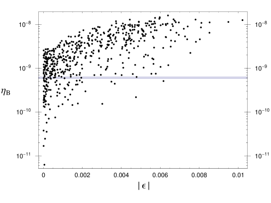
Figure 1: The predicted baryon asymmetry as a function of $|\epsilon|$ in the case $E$e6 with $b_{3}\neq 0$.

From the constraint of $\eta_{B}$, we have found that the value of $b_{3}$ should be of the order of $\mathcal{O}(0.1)-\mathcal{O}(1)$. In Figure. 1, we show the predicted value of $\eta_{B}$ as a function of $|\epsilon|$. Here we take the values of three right-handed Majorana masses $M_{i}$ $(i=1,2,3)$ as $M_{2}=5\times 10^{15}\sim 5\times 10^{16}~{}{\rm GeV},M_{1}=(0.01\sim 0.1)\times M_{2}$ and $M_{3}=(2\sim 10)\times M_{2}$. As we can see in Figure. 1, the order of magnitude of the breaking parameter $|\epsilon|$ in this case is given as $|\epsilon|=(b_{3}^{2}/b_{1}^{2})\times(M_{1}/M_{3})\simeq\mathcal{O}(10^{-5})\sim\mathcal{O}(10^{-3})$, which can only generate the very small values of $m_{3}\sim\mathcal{O}(10^{-9})-\mathcal{O}(10^{-6})$, $|U_{e3}|\sim\mathcal{O}(10^{-8})-\mathcal{O}(10^{-6})$ and $J_{CP}\sim\mathcal{O}(10^{-9})-\mathcal{O}(10^{-7})$. Thus, observation of $|U_{e3}|$ in the next generation of reactor and long-baseline neutrino experiments will exclude the case $E$e6 with $b_{3}\neq 0$.

For the case $E$e5 with $b_{1}\neq 0$ and the case $E$e6 with $b_{2}\neq 0$ (corresponding to the combination of the cases A2 and A3), we have

$$M_{D} = \left(\begin{array}[]{@{\,}ccc@{\,}}a_{1}e^{i\xi}&b_{1}e^{i\xi^{\prime}}&0\\ a_{2}&b_{2}&d_{2}\\ 0&0&0\end{array}\right)v\,,$$ (5.24)

$$M_{D}M_{D}^{\dagger} = \left(\begin{array}[]{@{\,}ccc@{\,}}a_{1}^{2}+b_{1}^{2}&a_{1}a_{2}e^{i\xi}+b_{1}b_{2}e^{i\xi^{\prime}}&0\\ a_{1}a_{2}e^{-i\xi}+b_{1}b_{2}e^{-i\xi^{\prime}}&a_{2}^{2}+b_{2}^{2}+d_{2}^{2}&0\\ 0&0&0\end{array}\right)v^{2}\,,$$ (5.28)

and

$$M_{D} = \left(\begin{array}[]{@{\,}ccc@{\,}}a_{1}&b_{1}&d_{1}\\ a_{2}e^{i\xi}&b_{2}e^{i\xi^{\prime}}&0\\ 0&0&0\end{array}\right)v\,,$$ (5.32)

$$M_{D}M_{D}^{\dagger} = \left(\begin{array}[]{@{\,}ccc@{\,}}a_{1}^{2}+b_{1}^{2}+d_{1}^{2}&a_{1}a_{2}e^{-i\xi}+b_{1}b_{2}e^{-i\xi^{\prime}}&0\\ a_{1}a_{2}e^{i\xi}+b_{1}b_{2}e^{i\xi^{\prime}}&a_{2}^{2}+b_{2}^{2}&0\\ 0&0&0\end{array}\right)v^{2}\,,$$ (5.36)

from which we can see that the correction from the breaking of the SSA does not affect on $\epsilon_{1}$ in the both cases as well as the $E$e5 with $b_{3}\neq 0$.

Table 6: The forms of $M_{D}$, $M_{D}M_{D}^{\dagger}$ and the CP asymmetry parameter $\epsilon_{i}$ for the class $E$ with the six conditions (e1)–(e6). Here, the case $E$e1 means the class $E$ with the condition (e1) and so on.

Case	$M_{D}/v$	$M_{D}M_{D}^{\dagger}/v^{2}$	$\epsilon_{i}$
$E$e1	$\left(\begin{array}[]{@{\,}ccc@{\,}}0&0&0\\ a_{2}e^{i\xi}&0&0\\ a_{3}&b_{3}&d_{3}\end{array}\right)^{\mathstrut}_{\mathstrut}$	$\left(\begin{array}[]{@{\,}ccc@{\,}}0&0&0\\ 0&a_{2}^{2}&a_{2}a_{3}e^{i\xi}\\ 0&a_{2}a_{3}e^{-i\xi}&a_{3}^{2}+b_{3}^{2}+d_{3}^{2}\end{array}\right)^{\mathstrut}_{\mathstrut}$	$\begin{array}[]{@{\,}c@{\,}}\epsilon_{2}=\frac{1}{8\pi_{\mathstrut}}a_{3}^{2}\sin(2\xi)f(M_{3}^{2}/M_{2}^{2})\\ \epsilon_{3}=\frac{-1}{8\pi}\frac{a_{2}^{2}a_{3}^{2}}{a_{3}^{2}+b_{3}^{2}+d_{3}^{2}}\sin(2\xi)f(M_{2}^{2}/M_{3}^{2})\end{array}$
$E$e2	$\left(\begin{array}[]{@{\,}ccc@{\,}}0&0&0\\ a_{2}&b_{2}&d_{2}\\ a_{3}e^{i\xi}&0&0\end{array}\right)^{\mathstrut}_{\mathstrut}$	$\left(\begin{array}[]{@{\,}ccc@{\,}}0&0&0\cr 0&a_{2}^{2}+b_{2}^{2}+d_{2}^{2}&a_{2}a_{3}e^{-i\xi}\cr 0&a_{2}a_{3}e^{i\xi}&a_{3}^{2}\end{array}\right)^{\mathstrut}_{\mathstrut}$	$\begin{array}[]{@{\,}c@{\,}}\epsilon_{2}=\frac{-1}{8\pi}\frac{a_{2}^{2}a_{3}^{2}}{a_{2}^{2}+b_{2}^{2}+d_{2}^{2}}\sin(2\xi)f(M_{3}^{2}/M_{2}^{2})\\ \epsilon_{3}=\frac{1^{\mathstrut}}{8\pi}a_{2}^{2}\sin(2\xi)f(M_{2}^{2}/M_{3}^{2})\end{array}$
$E$e3	$\left(\begin{array}[]{@{\,}ccc@{\,}}a_{1}e^{i\xi}&0&0\\ 0&0&0\\ a_{3}&b_{3}&d_{3}\end{array}\right)^{\mathstrut}_{\mathstrut}$	$\left(\begin{array}[]{@{\,}ccc@{\,}}a_{1}^{2}&0&a_{1}a_{3}e^{i\xi}\\ 0&0&0\\ a_{1}a_{3}e^{-i\xi}&0&a_{3}^{2}+b_{3}^{2}+d_{3}^{2}\end{array}\right)^{\mathstrut}_{\mathstrut}$	$\begin{array}[]{@{\,}c@{\,}}\epsilon_{1}=\frac{1}{8\pi_{\mathstrut}}a_{3}^{2}\sin(2\xi)f(M_{3}^{2}/M_{1}^{2})\\ \epsilon_{3}=\frac{-1}{8\pi}\frac{a_{1}^{2}a_{3}^{2}}{a_{3}^{2}+b_{3}^{2}+d_{3}^{2}}\sin(2\xi)f(M_{1}^{2}/M_{3}^{2})\end{array}$
$E$e4	$\left(\begin{array}[]{@{\,}ccc@{\,}}a_{1}&b_{1}&d_{1}\\ 0&0&0\\ a_{3}e^{i\xi}&0&0\end{array}\right)^{\mathstrut}_{\mathstrut}$	$\left(\begin{array}[]{@{\,}ccc@{\,}}a_{1}^{2}+b_{1}^{2}+d_{1}^{2}&0&a_{1}a_{3}e^{-i\xi}\\ 0&0&0\\ a_{1}a_{3}e^{i\xi}&0&a_{3}^{2}\end{array}\right)^{\mathstrut}_{\mathstrut}$	$\begin{array}[]{@{\,}c@{\,}}\epsilon_{1}=\frac{-1}{8\pi}\frac{a_{1}^{2}a_{3}^{2}}{a_{1}^{2}+b_{1}^{2}+d_{1}^{2}}\sin(2\xi)f(M_{3}^{2}/M_{1}^{2})\\ \epsilon_{3}=\frac{1^{\mathstrut}}{8\pi}a_{1}^{2}\sin(2\xi)f(M_{1}^{2}/M_{3}^{2})\end{array}$
$E$e5	$\left(\begin{array}[]{@{\,}ccc@{\,}}a_{1}e^{i\xi}&0&0\\ a_{2}&b_{2}&d_{2}\\ 0&0&0\end{array}\right)^{\mathstrut}_{\mathstrut}$	$\left(\begin{array}[]{@{\,}ccc@{\,}}a_{1}^{2}&a_{1}a_{2}e^{i\xi}&0\\ a_{1}a_{2}e^{-i\xi}&a_{2}^{2}+b_{2}^{2}+d_{2}^{2}&0\\ 0&0&0\end{array}\right)^{\mathstrut}_{\mathstrut}$	$\begin{array}[]{@{\,}c@{\,}}\epsilon_{1}=\frac{1}{8\pi_{\mathstrut}}a_{2}^{2}\sin(2\xi)f(M_{2}^{2}/M_{1}^{2})\\ \epsilon_{2}=\frac{-1}{8\pi}\frac{a_{1}^{2}a_{2}^{2}}{a_{2}^{2}+b_{2}^{2}+d_{2}^{2}}\sin(2\xi)f(M_{1}^{2}/M_{2}^{2})\end{array}$
$E$e6	$\left(\begin{array}[]{@{\,}ccc@{\,}}a_{1}&b_{1}&d_{1}\\ a_{2}e^{i\xi}&0&0\\ 0&0&0\end{array}\right)^{\mathstrut}_{\mathstrut}$	$\left(\begin{array}[]{@{\,}ccc@{\,}}a_{1}^{2}+b_{1}^{2}+d_{1}^{2}&a_{1}a_{2}e^{-i\xi}&0\\ a_{1}a_{2}e^{i\xi}&a_{2}^{2}&0\\ 0&0&0\end{array}\right)^{\mathstrut}_{\mathstrut}$	$\begin{array}[]{@{\,}c@{\,}}\epsilon_{1}=\frac{-1}{8\pi}\frac{a_{1}^{2}a_{2}^{2}}{a_{1}^{2}+b_{1}^{2}+d_{1}^{2}}\sin(2\xi)f(M_{2}^{2}/M_{1}^{2})\\ \epsilon_{2}=\frac{1^{\mathstrut}}{8\pi}a_{1}^{2}\sin(2\xi)f(M_{1}^{2}/M_{2}^{2})\end{array}$

Table 7: The allowed values of the parameters in $M_{D}$ and the predicted values of $\sin^{2}\theta_{23}$, $\sin^{2}\theta_{12}$, $\Delta m^{2}_{32}$, $\Delta m^{2}_{21}$ and $\langle m_{ee}\rangle$ in the cases $E$e5 and $E$e6.

	$E$e5	$E$e6
$a_{1}$	$0.46-0.59$	$0.019-0.023$
$a_{2}$	$0.17-0.24$	$6.6-8.8$
$b_{2}$	$1.2-1.8$	$1.4-2.0$
$d_{2}$	$1.1-1.5$	$1.1-1.9$
$\xi$	$\sim\pi/2,3\pi/2$	$\sim\pi/5,5\pi/6,5\pi/4,20\pi/11$
$\sin^{2}\theta_{23}$	$0.34-0.49$	$0.34-0.49$
$\sin^{2}\theta_{12}$	$0.26-0.40$	$0.26-0.39$
$\Delta m^{2}_{32}$	$2.2\times 10^{-3}-2.8\times 10^{-3}$	$2.0\times 10^{-3}-2.8\times 10^{-3}$
$\Delta m^{2}_{21}$	$7.2\times 10^{-5}-8.3\times 10^{-5}$	$7.1\times 10^{-5}-8.3\times 10^{-5}$
$\langle m_{ee}\rangle$	$0.046-0.052$	$0.044-0.052$

6 Summary

In this study, we have classified the Dirac and the right-handed Majorana neutrino mass matrices which can satisfy the SSA within the framework of the seesaw mechanism, assuming that the Dirac neutrino mass matrix has some texture zeros. We found that the resulting Dirac neutrino mass matrices have rank 2 as well as the rank of the effective neutrino mass matrix, or rank 1, depending only on the textures of $M_{R}^{-1}$. We also considered the three cases of breaking the SSA by introducing a complex breaking parameter in the neutrino mass matrix and examined the effects of the breaking of the SSA on $|U_{e3}|,m_{3}$ and $J_{CP}$.

We have calculated the baryon asymmetry of the universe in the cases $E$e5 and $E$e6 which satisfy the SSA in the basis where $M_{R}$ is diagonal. The implications of the baryon asymmetry for both cases are almost same. We have also discussed the implications of the baryon asymmetry in the case of the breaking of the SSA for the cases $E$e5 and $E$e6. We have found that only in the case $E$e6 with $b_{3}\neq 0$ ($d_{3}\neq 0$) corresponding to the case A2 (A1), the CP asymmetry parameter $\epsilon_{1}$ can receive the correction from the breaking of the SSA. From the constraint of the observed value of $\eta_{B}$, the order of magnitude of the breaking parameter $\epsilon$ should be of the order of $|\epsilon|\simeq\mathcal{O}(10^{-5})\sim\mathcal{O}(10^{-3})$, which can only generate the very small values of $m_{3}\sim\mathcal{O}(10^{-9})-\mathcal{O}(10^{-6})$, $|U_{e3}|\sim\mathcal{O}(10^{-8})-\mathcal{O}(10^{-6})$ and $J_{CP}\sim\mathcal{O}(10^{-9})-\mathcal{O}(10^{-7})$. Thus, observation of $|U_{e3}|$ in the next generation of reactor and long-baseline neutrino experiments will exclude the case $E$e6 with $b_{3}\neq 0$ ($d_{3}\neq 0$) as well as the original case of the SSA.

Appendix A Corrections for mass eigenvalues and eigenstates

In this appendix, we will list the explicite forms of the mass eigenvalues and mixing angles up to the next-leading and the leading order approximation of the diagonalization of Eq. (3.28), respectively. The leading and the next-leading order of corrections for mass eigenvalues $(m_{n}^{2})^{(1)}$’s and $(m_{n}^{2})^{(2)}$’s are given by

$$(m_{n}^{2})^{(1)} = \langle n^{(0)}|\delta\mathcal{M}|n^{(0)}\rangle\quad(n=1,2,3)\,,$$ (A.1)

$$(m_{n}^{2})^{(2)} = \sum_{k\neq n}\langle n^{(0)}|\delta\mathcal{M}|k^{(0)}\rangle\langle k^{(0)}|\delta\mathcal{M}|n^{(0)}\rangle\quad(n,k=1,2,3)\,,$$ (A.2)

and the leading order of corrections for mass eigenstates $|n^{(1)}\rangle$’s are given by

$$|n^{(1)}\rangle=\sum_{k\neq n}\frac{|k^{(0)}\rangle\langle k^{(0)}|\delta\mathcal{M}|n^{(0)}\rangle}{(m_{n}^{2})^{(0)}-(m_{k}^{2})^{(0)}}\quad(n,k=1,2,3)\,.$$ (A.3)

In the next three subsections, we will write down the corresponding expressions for Eqs. (A.1), (A.2) and (A.3) in the three cases A1, A2 and A3.

A.1 The case A1

In the case A1, the correction of the mass eigenvalues for the leading and the next-leading order of the approximation $(m_{n}^{2})^{(1)}$’s and $(m_{3}^{2})^{(2)}$ are given as follows :

$$(m_{1}^{2})^{(1)} = 2D^{2}\Biggr{(}1+\frac{2}{c^{2}}\Biggl{)}\cos(\phi-\varphi)|\epsilon|\sin^{2}\theta$$ (A.4)

$$- 2\frac{BD}{\sqrt{1+\frac{1}{c^{2}}}}\Biggr{(}1+\frac{2}{c^{2}}\Biggl{)}\cos\varphi|\epsilon|\sin\theta\cos\theta$$

$$+ D^{2}\Biggr{(}1+\frac{1}{c^{2}}+\frac{1}{1+c^{2}}\Biggl{)}|\epsilon|^{2}\sin^{2}\theta\,,$$

$$(m_{2}^{2})^{(1)} = 2D^{2}\Biggr{(}1+\frac{2}{c^{2}}\Biggl{)}\cos(\phi-\varphi)|\epsilon|\cos^{2}\theta$$ (A.5)

$$+ 2\frac{BD}{\sqrt{1+\frac{1}{c^{2}}}}\Biggr{(}1+\frac{2}{c^{2}}\Biggl{)}\cos\varphi|\epsilon|\sin\theta\cos\theta$$

$$+ D^{2}\Biggr{(}1+\frac{1}{c^{2}}+\frac{1}{1+c^{2}}\Biggl{)}|\epsilon|^{2}\cos^{2}\theta\,,$$

$$(m_{3}^{2})^{(1)} = \frac{D^{2}}{c^{2}(1+c^{2})}|\epsilon|^{2}\,,$$ (A.6)

$$(m_{3}^{2})^{(2)} = \frac{-1}{A^{\prime}D^{\prime}(1+c^{2})}\Biggl{[}\frac{B^{2}D^{2}D^{\prime}}{c^{4}}|\epsilon|^{2}$$ (A.7)

$$+ A^{\prime}D^{4}|\epsilon|^{2}\Biggr{(}\frac{1}{c^{4}}+\frac{2\cos(\phi-\varphi)}{c^{2}(1+c^{2})}|\epsilon|+\frac{1}{(1+c^{2})^{2}}|\epsilon|^{2}\Biggl{)}$$

$$+ 2\frac{BD^{3}B^{\prime}}{c^{2}}|\epsilon|^{2}\Biggr{(}\frac{\cos\varphi}{c^{2}}+\frac{\cos(\phi^{\prime}-\phi+\varphi)}{(1+c^{2})}|\epsilon|\Biggl{)}\Biggr{]}\,.$$

The forms of $\langle k^{(0)}|\delta\mathcal{M}|n^{(0)}\rangle$’s in Eq. (A.3) can be expressed as follows:

$$\langle 3^{(0)}|\delta\mathcal{M}|1^{(0)}\rangle = \frac{D^{2}}{c}\Biggr{(}\frac{e^{-i(\phi-\varphi)}}{c^{2}}+\frac{1}{1+c^{2}}|\epsilon|\Biggl{)}|\epsilon|\sin\theta$$ (A.8)

$$- \frac{BD}{c^{2}\sqrt{1+c^{2}}}e^{i(\phi^{\prime}-\phi+\varphi)}|\epsilon|\cos\theta$$

$$= \langle 1^{(0)}|\delta\mathcal{M}|3^{(0)}\rangle^{*}\,,$$ (A.9)

$$\langle 3^{(0)}|\delta\mathcal{M}|2^{(0)}\rangle = -\frac{D^{2}}{c}\Biggr{(}\frac{e^{-i(\phi-\varphi)}}{c^{2}}+\frac{1}{1+c^{2}}|\epsilon|\Biggl{)}|\epsilon|\cos\theta$$ (A.10)

$$- \frac{BD}{c^{2}\sqrt{1+c^{2}}}e^{i(\phi^{\prime}-\phi+\varphi)}|\epsilon|\sin\theta$$

$$= \langle 2^{(0)}|\delta\mathcal{M}|3^{(0)}\rangle^{*}\,,$$ (A.11)

$$\langle 2^{(0)}|\delta\mathcal{M}|1^{(0)}\rangle = -2\frac{D^{2}}{c^{2}}\Biggr{(}1+\frac{2}{c^{2}}\Biggl{)}\cos(\phi-\varphi)|\epsilon|\sin\theta\cos\theta$$ (A.12)

$$+ \frac{BD}{\sqrt{1+\frac{1}{c^{2}}}}\Biggr{(}1+\frac{2}{c^{2}}\Biggl{)}|\epsilon|(2\cos(\phi^{\prime}-\phi+\varphi)\cos^{2}\theta-e^{-i(\phi^{\prime}-\phi+\varphi)})$$

$$- D^{2}\Biggr{(}1+\frac{1}{c^{2}}\Biggl{)}|\epsilon|^{2}\sin\theta\cos\theta$$

$$= \langle 1^{(0)}|\delta\mathcal{M}|2^{(0)}\rangle^{*}\,.$$ (A.13)

Using Eqs. (3.39) and (3.40), we can obtain the correction of the three mixing angles for neutrinos as

$$(U_{\nu}^{(1)})_{e3} = -\frac{1}{A^{\prime}D^{\prime}\sqrt{1+\frac{1}{c^{2}}}}$$ (A.14)

$$\times \Biggl{[}\frac{D^{2}|B^{\prime}|}{c}e^{i\phi^{\prime}}\Biggr{(}\frac{e^{-i(\phi-\varphi)}}{c^{2}}+\frac{1}{1+c^{2}}|\epsilon|\Biggl{)}|\epsilon|-\frac{BDD^{\prime}}{c^{3}}e^{i(\phi-\varphi)}|\epsilon|\Biggr{]}\,,$$

$$(U_{\nu}^{(1)})_{\mu 3} = \frac{1}{A^{\prime}D^{\prime}(1+\frac{1}{c^{2}})^{3/2}}$$ (A.15)

$$\times \Biggl{[}\frac{A^{\prime}D^{2}}{c}\Biggl{(}\frac{e^{-i(\phi-\varphi)}}{c^{2}}+\frac{1}{1+c^{2}}|\epsilon|\Biggl{)}|\epsilon|-\frac{BD|B^{\prime}|}{c^{3}}e^{-i(\phi^{\prime}-\phi+\varphi)}|\epsilon|\Biggr{]}\,,$$

$$(U_{\nu}^{(1)})_{e2} = \frac{e^{i\phi^{\prime}}\cos\theta}{w}\Biggl{[}-2\frac{D^{2}}{c^{2}}\Biggr{(}1+\frac{2}{c^{2}}\Biggl{)}\cos(\phi-\varphi)|\epsilon|\sin\theta\cos\theta$$ (A.16)

$$+ \frac{BD}{\sqrt{1+\frac{1}{c^{2}}}}\Biggr{(}1+\frac{2}{c^{2}}\Biggl{)}|\epsilon|(2\cos(\phi^{\prime}-\phi+\varphi)\cos^{2}\theta-e^{i(\phi^{\prime}-\phi+\varphi)})$$

$$- D^{2}\Biggr{(}1+\frac{1}{c^{2}}\Biggl{)}|\epsilon|^{2}\sin\theta\cos\theta\Biggr{]}\,.$$

A.2 The case A2

In the case A2, the correction of the mass eigenvalues for the leading and the next-leading order of the approximation $(m_{n}^{2})^{(1)}$’s and $(m_{3}^{2})^{(2)}$ are given as follows :

$$(m_{1}^{2})^{(1)} = D^{2}\Biggr{(}2\cos\varphi+\frac{c^{2}}{1+c^{2}}|\epsilon|\Biggl{)}|\epsilon|\sin^{2}\theta$$ (A.17)

$$- 2\frac{BD}{\sqrt{1+\frac{1}{c^{2}}}}\cos(\phi^{\prime}-\phi+\varphi)|\epsilon|\sin\theta\cos\theta\,,$$

$$(m_{2}^{2})^{(1)} = D^{2}\Biggr{(}2\cos\varphi+\frac{c^{2}}{1+c^{2}}|\epsilon|\Biggl{)}|\epsilon|\cos^{2}\theta$$ (A.18)

$$+ 2\frac{BD}{\sqrt{1+\frac{1}{c^{2}}}}\cos(\phi^{\prime}-\phi+\varphi)|\epsilon|\sin\theta\cos\theta\,,$$

$$(m_{3}^{2})^{(1)} = \frac{D^{2}}{1+c^{2}}|\epsilon|^{2}\,,$$ (A.19)

$$(m_{3}^{2})^{(2)} = \frac{-1}{A^{\prime}D^{\prime}(1+\frac{1}{c^{2}})}\Biggl{[}\frac{B^{2}D^{2}D^{\prime}}{c^{2}}|\epsilon|^{2}+A^{\prime}D^{4}|\epsilon|^{2}\Biggr{(}\frac{1}{c^{2}}+\frac{2\cos\varphi}{1+c^{2}}|\epsilon|+\frac{c^{2}}{(1+c^{2})^{2}}|\epsilon|^{2}\Biggl{)}$$ (A.20)

$$- 2\frac{BD^{3}B^{\prime}}{c^{2}}|\epsilon|^{2}\Biggr{(}\cos(\phi^{\prime}+\varphi)+\frac{c^{2}}{(1+c^{2})^{2}}\cos(\phi^{\prime}-\phi+\varphi)|\epsilon|\Biggl{)}\Biggr{]}\,.$$

The forms of $\langle k^{(0)}|\delta\mathcal{M}|n^{(0)}\rangle$’s in Eq. (A.3) can be expressed as follows:

$$\langle 3^{(0)}|\delta\mathcal{M}|1^{(0)}\rangle = \frac{D^{2}}{c}\Biggr{(}e^{i\varphi}+\frac{c^{2}}{1+c^{2}}|\epsilon|\Biggl{)}|\epsilon|\sin\theta$$ (A.21)

$$- \frac{BD}{\sqrt{1+c^{2}}}e^{i(\phi^{\prime}-\phi+\varphi)}|\epsilon|\cos\theta$$

$$= \langle 1^{(0)}|\delta\mathcal{M}|3^{(0)}\rangle^{*}\,,$$ (A.22)

$$\langle 3^{(0)}|\delta\mathcal{M}|2^{(0)}\rangle = -\frac{D^{2}}{c}\Biggr{(}e^{i\varphi}+\frac{c^{2}}{1+c^{2}}|\epsilon|\Biggl{)}|\epsilon|\cos\theta$$ (A.23)

$$- \frac{BD}{\sqrt{1+c^{2}}}e^{i(\phi^{\prime}-\phi+\varphi)}|\epsilon|\sin\theta$$

$$= \langle 2^{(0)}|\delta\mathcal{M}|3^{(0)}\rangle^{*}\,,$$ (A.24)

$$\langle 2^{(0)}|\delta\mathcal{M}|1^{(0)}\rangle = -D^{2}\Biggr{(}2\cos\varphi+\frac{c^{2}}{1+c^{2}}|\epsilon|\Biggl{)}|\epsilon|\sin\theta\cos\theta$$ (A.25)

$$+ \frac{BD}{\sqrt{1+\frac{1}{c^{2}}}}|\epsilon|(2\cos(\phi^{\prime}-\phi+\varphi)\cos^{2}\theta-e^{-i(\phi^{\prime}-\phi+\varphi)})$$

$$= \langle 1^{(0)}|\delta\mathcal{M}|2^{(0)}\rangle^{*}\,.$$ (A.26)

Using Eqs. (3.39) and (3.40), we can obtain the correction of the three mixing angles for neutrinos as

$$(U_{\nu}^{(1)})_{e3} = \frac{-1}{A^{\prime}D^{\prime}\sqrt{1+\frac{1}{c^{2}}}}$$ (A.27)

$$\times \Biggl{[}\frac{D^{2}|B^{\prime}|}{c}e^{i\phi^{\prime}}\Biggl{(}e^{-i\varphi}+\frac{c^{2}}{1+c^{2}}|\epsilon|\Biggl{)}|\epsilon|-\frac{BDD^{\prime}}{c}e^{i(\phi-\varphi)}|\epsilon|\Biggr{]}\,,$$

$$(U_{\nu}^{(1)})_{\mu 3} = \frac{1}{A^{\prime}D^{\prime}(1+\frac{1}{c^{2}})^{3/2}}$$ (A.28)

$$\times \Biggl{[}\frac{A^{\prime}D^{2}}{c}\Biggl{(}e^{-i\varphi}+\frac{c^{2}}{1+c^{2}}|\epsilon|\Biggl{)}|\epsilon|-\frac{BD|B^{\prime}|}{c}e^{-i(\phi^{\prime}-\phi+\varphi)}|\epsilon|\Biggr{]}\,,$$

$$(U_{\nu}^{(1)})_{e2} = \frac{e^{i\phi^{\prime}}\cos\theta}{w}\Biggl{[}-D^{2}\Biggr{(}2\cos\varphi+\frac{c^{2}}{1+c^{2}}|\epsilon|\Biggl{)}|\epsilon|\sin\theta\cos\theta$$ (A.29)

$$+ \frac{BD}{\sqrt{1+\frac{1}{c^{2}}}}|\epsilon|(2\cos(\phi^{\prime}-\phi+\varphi)\cos^{2}\theta-e^{i(\phi^{\prime}-\phi+\varphi)})\Biggr{]}\,.$$

A.3 The case A3

In the case A3, the correction of the mass eigenvalues for the leading and the next-leading order of the approximation $(m_{n}^{2})^{(1)}$’s and $(m_{3}^{2})^{(2)}$ are given as follows :

$$(m_{1}^{2})^{(1)} = 2B^{2}|\epsilon|\cos^{2}\theta+2B^{2}|\epsilon|\cos\varphi\sin^{2}\theta$$ (A.30)

$$- 2BD\sqrt{1+\frac{1}{c^{2}}}\cos(\phi^{\prime}-\phi^{\prime\prime})|\epsilon|\sin\theta\cos\theta$$

$$- 2\frac{AB}{\sqrt{1+\frac{1}{c^{2}}}}\cos(\phi^{\prime}+\phi^{\prime\prime})|\epsilon|\sin\theta\cos\theta$$

$$+ B^{2}\frac{c^{2}}{1+c^{2}}|\epsilon|^{2}\sin^{2}\theta+B^{2}|\epsilon|^{2}\cos^{2}\theta\,,$$

$$(m_{2}^{2})^{(1)} = 2B^{2}|\epsilon|\sin^{2}\theta+2B^{2}|\epsilon|\cos\varphi\cos^{2}\theta$$ (A.31)

$$+ 2BD\sqrt{1+\frac{1}{c^{2}}}\cos(\phi^{\prime}-\phi^{\prime\prime})|\epsilon|\sin\theta\cos\theta$$

$$+ 2\frac{AB}{\sqrt{1+\frac{1}{c^{2}}}}\cos(\phi^{\prime}+\phi^{\prime\prime})|\epsilon|\sin\theta\cos\theta$$

$$+ B^{2}\frac{c^{2}}{1+c^{2}}|\epsilon|^{2}\cos^{2}\theta+B^{2}|\epsilon|^{2}\sin^{2}\theta\,,$$

$$(m_{3}^{2})^{(1)} = \frac{B^{2}}{1+c^{2}}|\epsilon|^{2}\,,$$ (A.32)

$$(m_{3}^{2})^{(2)} = \frac{-1}{A^{\prime}D^{\prime}(1+\frac{1}{c^{2}})}\Biggl{[}\frac{A^{2}B^{2}D^{\prime}}{c^{2}}|\epsilon|^{2}+A^{\prime}B^{4}|\epsilon|^{2}\Biggr{(}\frac{1}{c^{2}}+\frac{2\cos\varphi}{1+c^{2}}|\epsilon|+\frac{c^{2}}{(1+c^{2})^{2}}|\epsilon|^{2}\Biggl{)}$$ (A.33)

$$- 2\frac{AB^{3}B^{\prime}}{c^{2}}|\epsilon|^{2}\Biggr{(}\cos(\phi^{\prime}+\varphi)+\frac{c^{2}}{1+c^{2}}\cos(\phi^{\prime}-\phi+\varphi)|\epsilon|\Biggl{)}\Biggr{]}\,,$$

where $\phi^{\prime\prime}=\phi+\varphi$.

The forms of $\langle k^{(0)}|\delta\mathcal{M}|n^{(0)}\rangle$’s in Eq. (A.3) can be expressed as follows:

$$\langle 3^{(0)}|\delta\mathcal{M}|1^{(0)}\rangle = \frac{B^{2}}{c}\Biggr{(}e^{i\varphi}+\frac{c^{2}}{1+c^{2}}|\epsilon|\Biggl{)}|\epsilon|\sin\theta$$ (A.34)

$$- \frac{AB}{\sqrt{1+c^{2}}}e^{i(\phi^{\prime}+\phi^{\prime\prime})}|\epsilon|\cos\theta$$

$$= \langle 1^{(0)}|\delta\mathcal{M}|3^{(0)}\rangle^{*}\,,$$ (A.35)

$$\langle 3^{(0)}|\delta\mathcal{M}|2^{(0)}\rangle = -\frac{B^{2}}{c}\Biggr{(}e^{i\varphi}+\frac{c^{2}}{1+c^{2}}|\epsilon|\Biggl{)}|\epsilon|\cos\theta$$ (A.36)

$$- \frac{AB}{\sqrt{1+c^{2}}}e^{i(\phi^{\prime}+\phi^{\prime\prime})}|\epsilon|\sin\theta$$

$$= \langle 2^{(0)}|\delta\mathcal{M}|3^{(0)}\rangle^{*}\,,$$ (A.37)

$$\langle 2^{(0)}|\delta\mathcal{M}|1^{(0)}\rangle = 2B^{2}(1-\cos\varphi)|\epsilon|\sin\theta\cos\theta+B^{2}\frac{1}{1+c^{2}}|\epsilon|^{2}\sin\theta\cos\theta$$ (A.38)

$$+ BD\sqrt{1+\frac{1}{c^{2}}}|\epsilon|(2\cos(\phi^{\prime}-\phi^{\prime\prime})\cos^{2}\theta-e^{-i(\phi^{\prime}-\phi^{\prime\prime})})$$

$$+ \frac{AB}{\sqrt{1+\frac{1}{c^{2}}}}|\epsilon|(2\cos(\phi^{\prime}+\phi^{\prime\prime})\cos^{2}\theta-e^{-i(\phi^{\prime}+\phi^{\prime\prime})})$$

$$= \langle 1^{(0)}|\delta\mathcal{M}|2^{(0)}\rangle^{*}\,.$$ (A.39)

Using Eqs. (3.39) and (3.40), we can obtain the correction of the three mixing angles for neutrinos as

$$(U_{\nu}^{(1)})_{e3} = \frac{1}{A^{\prime}D^{\prime}\sqrt{1+\frac{1}{c^{2}}}}$$ (A.40)

$$\times \Biggl{[}-\frac{B^{2}|B^{\prime}|}{c}e^{i\phi^{\prime}}\Biggl{(}e^{-i\varphi}+\frac{c^{2}}{1+c^{2}}|\epsilon|\Biggl{)}|\epsilon|+\frac{ABD^{\prime}}{c}e^{-i\phi^{\prime\prime}}|\epsilon|\Biggr{]}\,,$$

$$(U_{\nu}^{(1)})_{\mu 3} = \frac{1}{A^{\prime}D^{\prime}(1+\frac{1}{c^{2}})^{3/2}}$$ (A.41)

$$\times \Biggl{[}\frac{A^{\prime}B^{2}}{c}\Biggl{(}e^{-i\varphi}+\frac{c^{2}}{1+c^{2}}|\epsilon|\Biggl{)}|\epsilon|-\frac{AB|B^{\prime}|}{c}e^{-i(\phi^{\prime}+\phi^{\prime\prime})}|\epsilon|\Biggr{]}\,,$$

$$(U_{\nu}^{(1)})_{e2} = \frac{e^{i\phi^{\prime}}\cos\theta}{w}\Biggl{[}2B^{2}(1-\cos\varphi)|\epsilon|\sin\theta\cos\theta+B^{2}\frac{1}{1+c^{2}}|\epsilon|^{2}\sin\theta\cos\theta$$ (A.42)

$$+ BD\sqrt{1+\frac{1}{c^{2}}}|\epsilon|(2\cos(\phi^{\prime}-\phi^{\prime\prime})\cos^{2}\theta-e^{i(\phi^{\prime}-\phi^{\prime\prime})})$$

$$+ \frac{AB}{\sqrt{1+\frac{1}{c^{2}}}}|\epsilon|(2\cos(\phi^{\prime}+\phi^{\prime\prime})\cos^{2}\theta-e^{i(\phi^{\prime}+\phi^{\prime\prime})})\Biggr{]}\,.$$

References

- [1] Super-Kamiokande Collaboration, Y. Fukuda et al., Phys. Rev. Lett. 81, 1562 (1998); Y. Ashie et al., Phys. Rev. Lett. 93, 101801 (2004).
- [2] SNO Collaboration, Q.R. Ahmad et al., Phys. Rev. Lett. 87, 071301 (2001); Phys. Rev. Lett. 92, 181301 (2004).
- [3] KamLAND Collaboration, K. Eguchi et al., Phys. Rev. Lett. 90, 021802 (2003); T. Araki et al., Phys. Rev. Lett. 94, 081801 (2005).
- [4] K2K Collaboration, M.H. Ahn et al., Phys. Rev. Lett. 90, 041801 (2003); Phys. Rev. Lett. 94, 081802 (2005).
- [5] MINOS Collaboration, G.D. Michael et al., Phys. Rev. D 97, 191801 (2006); arXiv:0708.1495 [hep-ex].
- [6] M. Maltoni, T. Schwetz, M.A. Tortola, J.W.F. Valle, New J.Phys. 6, 122 (2004) [hep-ph/0405172 (v6)].
- [7] For reviews, see, e.g., G. Altarelli and F. Feruglio, New J. Phys. 6, 106 (2004); R.N. Mohapatra and A.Y. Smirnov, Ann. Rev. Nucl. Part. Sci. 56, 569 (2006).
- [8] For reviews, see, e.g., A. Mondragon, AIP Conf. Proc. 857B, 266 (2006).
- [9] For reviews, see, e.g., M.C. Chen and K.T. Mahanthappa, Int. J. Mod. Phys. A 18, 5819 (2003); S.F. King, Rept. Prog. Phys. 67, 107 (2004); See also, Ref. [7].
- [10] R.N. Mohapatra and W. Rodejohann, Phys. Lett. B 644, 59 (2007).
- [11] N.N. Singh, H.Z. Devi and M. Patgiri, arXiv:0707.2713 [hep-ph].
- [12] S.M. Bilenky, J. Hosek and S.T. Petcov, Phys. Lett. B 94, 495 (1980); J. Schechter and J.W.F. Valle, Phys. Rev. D 22, 2227 (1980); Phys. Rev. D 23, 1666 (1981); M. Doi et al., Phys. Lett. B 102, 323 (1981); Yu.F. Pirogov, Eur. Phys. J. C 17, 407 (2000).
- [13] A. Blum, R.N. Mohapatra and W. Rodejohann, arXiv:0706.3801 [hep-ph].
- [14] S. Kaneko and M. Tanimoto, Phys. Lett. B 551, 127 (2003).
- [15] G.C. Branco, R. Gonzalez Felipe, F.R. Joaquim, I. Masina, M.N. Rebelo and C.A. Savoy, Phys. Rev. D 67, 073025 (2003).
- [16] For the case of two right-handed heavy neutrinos, A. Ibarra, G.G. Ross, Phys. Lett. B 591, 285 (2004); W.l. Guo, Z.z. Xing and S. Zhou, Int. J. Mod. Phys. E 16, 1 (2007), and references therein.
- [17] G.C. Branco, M.N. Rebelo, J.I. Silva-Marcos, Phys. Lett. B 633, 345 (2006); G.C. Branco, D. Emmanuel-Costa, M.N. Rebelo and P. Roy, arXiv:0712.0774 [hep-ph].
- [18] Y. Koide and E. Takasugi, arXiv:0706.4373 [hep-ph].
- [19] M. Fukugita and T. Yanagida. Phys. Lett. B 175, 45 (1986).
- [20] T. Endoh, T. Morozumi, Z. Xiong, Prog. Theor. Phys. 111, 123 (2004); T. Fujihara, S. Kaneko, S. Kang, D. Kimura, T. Morozumi, M. Tanimoto, Phys. Rev. D 72, 016006 (2005); A. Abada, S. Davidson, F-X.J. Michaux, M. Losada and A. Riotto, JCAP 0604, 004 (2006); E. Nardi, Y. Nir, E. Roulet and J. Racker, JHEP 0601, 164 (2006); A. Abada, S. Davidson, A. Ibarra, F.X. Josse-Michaux, M. Losada and A. Riotto, JHEP 0609, 010 (2006); S. Blanchet and P.Di Bari, JCAP 0703, 018 (2007); S. Antusch, S.F. King and A. Riotto, JCAP 0611, 011 (2006); S. Pascoli, S.T. Petcov and A. Riotto, Phys. Rev. D 75, 083511 (2007); S. Pascoli, S.T. Petcov and A. Riotto, Nucl. Phys. B 774, 1 (2007); G.C. Branco, R. Gonzalez Felipe and F.R. Joaquim, Phys. Lett. B 645, 432 (2007); G.C. Branco, A.J. Buras, S. Jager, S. Uhlig and A. Weiler, JHEP 0709, 004 (2007); S. Antusch and A.M. Teixeira, JCAP 0702, 024 (2007).
- [21] W. Buchmuller, P. Di Bari and M. Plumacher, Nucl. Phys. B 643, 367 (2002); Phys. Lett. B 547, 128 (2002); G.F. Giudice, A. Notari, M. Raidal, A. Riotto and A. Strumia, Nucl. Phys. B 685, 89 (2004); See also, M.Y. Khlopov and A.D. Linde, Phys. Lett. B 138, 265 (1984); F. Balestra and G. Piragino, G.B. Pontecorvo, M.G. Sapozhnikov, I.V. Falomkin and M.Y. Khlopov, Sov. J. Nucl. Phys. 39, 626 (1984); M.Y. Khlopov, Yu.L. Levitan, E.V. Sedelnikov and I.M. Sobol, Phys. Atom. Nucl. 57, 1393 (1994).
- [22] L. Covi, E. Roulet and F. Vissani, Phys. Lett. B 384, 169 (1996).
- [23] M. Luty, Phys. Rev. D 45, 1992 (455); M. Plümacher, Z. Phys. C 74, 549 (1997); E.W. Kolb and M. S. Turner, The early universe, Redwood City, USA: Addison-Wesley (1990), (Frontiers in physics, 69); M. Flanz and E.A. Paschos, Phys. Rev. D 58, 113009 (1998).
- [24] W. Buchmüller, P. Di Bari and M. Plümacher, Annals of Physics 315, 305 (2005).
- [25] H.B. Nielsen and Y. Takanishi, Phys. Lett. B 507, 241 (2001).
- [26] WMAP Collaboration, D.N. Spergel et al., Aastrophys. J. Suppl. 170, 377 (2007).