SU(3) Deconfining Phase Transition in a Box with Cold Boundaries

Abstract:

Deconfined regions created in heavy ion collisions are bordered by the confined phase. We discuss boundary conditions (BCs) to model a cold exterior. Monte Carlo simulations of pure SU(3) lattice gauge theory with thus inspired BCs show scaling. Corrections to usual results survive in the finite volume continuum limit and we estimate them in a range from $L=5-10$ fermi as function of the volume size $L^{3}$. In magnitude these corrections are comparable to those obtained by including quarks.

1 Introduction

Past LGT simulations of the deconfining transition focused primarily on boundary conditions (BCs), which are favorable for reaching the infinite volume quantum continuum limit (thermodynamic limit of the textbooks) quickly. On $N_{\tau}\,N_{s}^{3}$ lattices these are periodic BCs in the spatial volume $V=(a\,N_{s})^{3}$, where $a$ is the lattice spacing. The temperature of the system is given by

$$T=\frac{1}{a\,N_{\tau}}=\frac{1}{L_{\tau}}\,,~{}~{}~{}(N_{\tau}<N_{s})\ .$$ (1)

In the following we set the physical scale by

$$T^{c}=174\ {\rm MeV}\ ,$$ (2)

which is approximately the average from QCD estimates with two light flavor quarks. This implies for the temporal extension

$$L_{\tau}=a\,N_{\tau}=1.13\ {\rm fermi}\ .$$ (3)

For the deconfinement phase created in a heavy ion collision the infinite volume limit does not apply. Instead we have to take the finite volume continuum limit

$$N_{s}/N_{\tau}={\rm finite}\,,~{}~{}N_{\tau}\to\infty\,,~{}~{}L_{\tau}~{}~{}{\rm finite}\,,$$ (4)

and periodic BCs are incorrect, because the outside is in the confined phase at low temperature. E.g., at the BNL RHIC one expects to create an ensemble of differently shaped and sized deconfined volumes. The largest volumes are those encountered in central collisions. A rough estimate of their size is

$$\pi\times(0.6\times{\rm Au\ radius})^{2}\times c\times({\rm expansion\ time})$$

$$=(55\ {\rm fermi}^{2})\times({\rm a\ few\ fermi})$$ (5)

where $c$ is the speed of light. Here we report on our work [1], which estimates such finite volume corrections for pure SU(3) and focuses on the continuum limit for

$$L_{s}=aN_{s}=(5-10)\ {\rm fermi}\ .$$ (6)

2 Equilibrium with Unconventional Boundary Conditions

Statistical properties of a quantum system with Hamiltonian $H$ in a continuum volume $V$, which is in equilibrium with a heatbath at physical temperature $T$, are determined by the partition function

$$Z(T,V)={\rm Tr}e^{-H/T}=\sum_{\phi}\langle\phi|e^{-H/T}|\phi\rangle,$$ (7)

where the sum extends over all states and the Boltzmann constant is set to one. Imposing periodic boundary conditions in Euclidean time $\tau$ and bounds of integration from $0$ to $1/T$, one can rewrite the partition function in the path integral representation:

$$Z(T,V)=\int D\phi\exp\left\{-\int_{0}^{1/T}d\tau L_{E}(\phi,\dot{\phi})\right\}.$$ (8)

Nothing in this formulation requires to carry out the infinite volume limit.

In the following we consider difficulties and effects encountered when one equilibrates a hot volume with cold boundaries by means of Monte Carlo (MC) simulations for which the updating process provides the equilibrium. We use the single plaquette Wilson action on a 4D hypercubic lattice. Numerical evidence suggests that SU(3) lattice gauge theory exhibits a weakly first-order deconfining phase transition at some coupling $\beta^{g}_{t}(N_{\tau})=6/g^{2}_{t}(N_{\tau})$. The scaling behavior of the deconfining temperature is

$$T^{c}=c_{T}\,\Lambda_{L}$$ (9)

where the lambda lattice scale

$$a\,\Lambda_{L}=f_{\lambda}(\beta^{g})=\lambda(g^{2})\,\left(b_{0}\,g^{2}\right)^{-b_{1}/(2b_{0}^{2})}\,e^{-1/(2b_{0}\,g^{2})}\,,$$ (10)

has been determined in the literature. The coefficients $b_{0}$ and $b_{1}$ are perturbatively determined by the renormalization group equation:

$$b_{0}=\frac{11}{3}\frac{3}{16\pi^{2}}~{}~{}{\rm and}~{}~{}b_{1}=\frac{34}{3}\left(\frac{3}{16\pi^{2}}\right)^{2}\,.$$ (11)

Relying on work by the Bielefeld group [2] we parametrized in [3] higher perturbative and non-perturbative corrections by

$$\lambda(g^{2})\ =\ 1+a_{1}\,e^{-a_{2}/g^{2}}+a_{3}\,g^{2}+a_{4}\,g^{4}~{}~{}~{}{\rm with}$$ (12)

$a_{1}=71553750,\ a_{2}=19.48099,\ a_{3}=-0.03772473,\ a_{4}=0.5089052$, which turns out to be in good agreement with [4] in the coupling constant range for which the latter is claimed to be valid.

Imagine an almost infinite space volume $V=L_{s}^{3}$, which may have periodic BCs, and a smaller (very large, but small compared to $V$) sub-volume $V_{0}=L_{s,0}^{3}.$ The complement to $V_{0}$ in $V$ will be called $V_{1}$. The number of temporal lattice links $N_{\tau}$ is the same for both volumes. We denote the coupling by $\beta^{g}_{0}$ for plaquettes in $V_{0}$ and by $\beta^{g}_{1}$ for plaquettes in $V_{1}$. For that purpose any plaquette touching a site in $V_{1}$ is considered to be in $V_{1}$. This defines a BC, which we call disorder wall.

We would like to find couplings so that scaling holds, while $V_{0}$ is at temperature $T_{0}=174\,{\rm MeV}$ and $V_{1}$ at room temperature $T_{1}$. Let us take $\beta^{g}_{1}=5.7$ at the beginning of the SU(3) scaling region. We have

$$10^{10}\approx\frac{T_{0}}{T_{1}}=\frac{a_{1}}{a_{0}}=\frac{f_{\lambda}(\beta^{g}_{1})}{f_{\lambda}(\beta^{g}_{0})}$$ (13)

where $a_{i}$ is the lattice spacing in $V_{i},\,i=0,1$. Using the lambda scale yields $\beta^{g}_{0}\approx 25$ and $T_{c}$ estimates of the literature give $L_{\tau}>10^{11}\,a$. In practice we can only have $\beta^{g}_{0}$ in the scaling region. We keep up the relation

$$\frac{(\xi/a_{0})}{(\xi/a_{1})}=\frac{a_{1}}{a_{0}}\approx 10^{10}$$ (14)

where $\xi$ is a correlation length. Therefore, $\xi/a_{1}$ is very small and the strong coupling expansion implies $\beta^{g}_{1}\approx 10^{-10^{10}}$, i.e., $\beta^{g}_{1}=0$.

3 Monte Carlo Calculations with Disorder Wall BCs

In the disorder wall approximation of the cold exterior we can simply omit contributions from plaquettes, which involve links through the boundary. Due to the use of the strong coupling limit for the BCs, scaling of the results is not obvious.

We use the maxima of the Polyakov loop susceptibility

$$\chi_{\max}=\frac{1}{N_{s}^{3}}\left[\langle|P|^{2}\rangle-\langle|P|\rangle^{2}\right]_{\max},\,\,\,P=\sum_{\vec{x}}P_{\vec{x}}$$ (15)

to define pseudo-transition couplings $\beta^{g}_{pt}(N_{s};N_{\tau})$. For periodic BCs they have a finite size behavior of the form

$$\beta^{g}_{pt}(N_{s};N_{\tau})=\beta^{g}_{t}(N_{\tau})+a_{3}^{p}\,\left(\frac{N_{\tau}}{N_{s}}\right)^{3}+\ \dots\ .$$ (16)

Our BCs introduce an order $N_{s}^{2}$ disturbance, so that

$$\beta^{g}_{pt}(N_{s};N_{\tau})=\beta^{g}_{t}(N_{\tau})+a_{1}^{d}\,\frac{N_{\tau}}{N_{s}}+a_{2}^{d}\,\left(\frac{N_{\tau}}{N_{s}}\right)^{2}+a_{3}^{d}\,\left(\frac{N_{\tau}}{N_{s}}\right)^{3}+\ \dots\ .$$ (17)

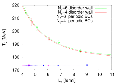
Figure 1: Fits of pseudo-transition coupling constant values (left). Estimate of finite volume corrections to $T_{c}$ (right).

The left Fig. 1 shows thus obtained fits of pseudo-transition coupling constant values versus $N_{\tau}/N_{s}$ (the $N_{s}\to\infty$ value is extrapolated from simulations with periodic BCs). Using the scaling relation (10) we eliminate the coupling in favor of $T_{c}$ and $L_{s}$ and obtain the right Fig. 1. There are no free parameters in this step, because the scaling relation was determined previously in independent work. The $N_{\tau}=4$ and $N_{\tau}=6$ data collapse to one curve, i.e., despite the small values of the temporal lattice sizes the results are perfectly consistent with scaling.

Figure 2: Polyakov loop susceptibility with disorder wall BCs on a $4\times 16^{3}$ lattice (left). Fits of the $N_{\tau}=4$ widths (right).

The left Fig. 2 shows the Polyakov loop susceptiblity on a $4\times 16^{4}$ lattice with disorder BCs and its full width at 2/3 maximum, which we used instead of the more conventional full width at half maximum, because the former is easier to extract from MC data (smaller reweighting range). Our width data are fitted to the form

$$\Delta\beta^{g}_{2/3}=c_{1}^{p}\left(\frac{N_{\tau}}{N_{s}}\right)^{3}+c_{2}^{p}\left(\frac{N_{\tau}}{N_{s}}\right)^{6}$$ (18)

for periodic BCs and to

$$\Delta\beta^{g}_{2/3}=c_{1}^{d}\left(\frac{N_{\tau}}{N_{s}}\right)^{3}+c_{2}^{d}\left(\frac{N_{\tau}}{N_{s}}\right)^{4}$$ (19)

for disorder wall BCs. The first term reflects in both cases the delta function singularity of a first order phase transition, i.e., the width times the Polyakov loop maximum is supposed to approach a constant for $N_{s}\to\infty$. The leading order correction to that is 1/Volume for periodic BCs and $1/N_{s}$ for disorder wall BCs. Plots of the corresponding fits are shown in Figs. 2 (right) and 3 (left). As before, we use the scaling relation (10) to eliminate the coupling constant and show in Fig. 3 (right) the thus obtained volume dependence of the width of the transition. Again, we see collapse to a nice scaling curve.

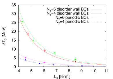
Figure 3: Fits of the $N_{\tau}=6$ widths (left). Estimate of finite volume corrections to the width (right).

4 Shortcomings of the Disorder Wall BCs

The spatial lattice spacing $a_{s}$ should be the same on both sides of the boundary, but for the disorder wall this is not true. It reflects the temperature jump at the price of introducing a similar jump in the spatial lattice spacing. Its main advantage that it allows for technically simple simulations, and one can hope that the temperature jump is the only relevant quantity for the questions asked.

A construction, called confinement wall in [1], for which the physical length of one spacelike lattice spacing stays constant across the boundary can be achieved by using an anisotropic lattice for the volume $V_{1}$:

$$S(\{U\})=\frac{\beta^{g}_{s}}{3}\sum_{{\Box}_{s}}{\rm Re}\,{\rm Tr}\left(U_{{\Box}_{s}}\right)+\frac{\beta^{g}_{\tau}}{3}\sum_{{\Box}_{\tau}}{\rm Re}\,{\rm Tr}\left(U_{{\Box}_{\tau}}\right)\,.$$ (20)

The lambda scale of this action has been investigated by Karsch [5] and in the continuum limit one finds

$$\beta^{g}_{\tau}/\beta^{g}_{s}=\left(a_{s}/a_{\tau}\right)^{2}\,.$$ (21)

When we aim at $a_{0}=a_{s}\approx 10^{-10}\,a_{\tau}$ the sublattice $V_{1}$ is driven to $\beta^{g}_{\tau}=0$ and the simulation of the confined world becomes effectively 3D. However, in a first step one may be content with a temperature slightly below $T_{c}$ on the outside, so that the confinement wall allows to have all $\beta$-values in their scaling regions. Another approach may want to rely on symmetric lattices to model low temperatures.

5 Summary and Conclusions

1. As noted before [2] finite size corrections to deconfinement properties of SU(3) are very small for periodic BCs.

2. For volumes of BNL RHIC size the magnitudes of SU(3) corrections due to cold boundaries appear to be comparable to those of including quarks into pure SU(3) LGT. Our data show the correct SU(3) scaling behavior.

3. Extension of measurements should be done, to calculate the equation of state.

4. Previous calculations [6, 7] of full QCD at finite temperatures and RHIC (low) densities should be extended to other than periodic BCs.

5. There appears to be a variety of options to include cold boundaries and approaching the finite volume continuum limit. Therefore, more experience with pure SU(3) LGT is desirable before including quarks. Next, we intend to focus on the confinement wall with both couplings in the scaling region (i.e., an outside temperature just below $T_{c}$).

- [1] A. Bazavov and B.A. Berg, Phys. Rev. D 76 (2007) 014502, hep-lat/0701007.
- [2] G. Boyd, J. Engels, F. Karsch, E. Laermann, C. Legeland, M. Lütgemeier, and B. Petersson, Nucl. Phys. B 469 (1996) 419.
- [3] A. Bazavov, B.A. Berg, and A. Velytsky, Phys. Rev. D 74 (2006) 014501.
- [4] S. Necco and R. Sommer, Nucl. Phys. B 622 (2002) 328.
- [5] F. Karsch, Nucl. Phys. B 205 (1982) 285.
- [6] Z. Fodor, these proceedings, arXiv:0711.0336[hep-lat].
- [7] F. Karsch, these proceedings.