Quantum cosmology with varying speed of light: canonical approach

Abstract

We investigate $(n+1)$–dimensional cosmology with varying speed of light. After solving corresponding Wheeler-DeWitt equation, we obtain exact solutions in both classical and quantum levels for ($c\,$–$\Lambda$)–dominated Universe. We then construct the “canonical” wave packets which exhibit a good classical and quantum correspondence. We show that arbitrary but appropriate initial conditions lead to the same classical description. We also study the situation from de-Broglie Bohm interpretation of quantum mechanics and show that the corresponding Bohmian trajectories are in good agreement with the classical counterparts.

1 Introduction

In recent years the varying speed of light theories (VSL) have attracted much attentions [1, 2, 3, 4, 5, 6, 7, 8, 9, 10, 11, 12, 13, 14, 15, 16, 17, 18] (for a comprehensive review see [19]). These theories proposed by Moffat [1] and Albrecht and Magueijo [2], in which light is traveling faster in the early periods of the existence of the Universe, could be considered as an alternative to the inflation scenario. It has been shown that the horizon, flatness, and cosmological constant problems can be solved in these models. Moreover, homogeneity and isotropy problems may find their appropriate solutions through this mechanism [2]. Recently, an interesting discussion on the foundations of VSL theories and the conceptual problems arising from the meaning of varying speed of light have been done by Ellis, Magueijo and Moffat [20, 21].

It is shown that it is possible to generalize these ideas to preserve the general covariance and local lorentz invariance [22]. They have the merit of retaining only those aspects of the usual definitions that are invariant under unit transformations and which can therefore represent the outcome of an experiment. This can be done by introducing a time-like coordinate $x^{0}$ which is not necessarily equal to $ct$. In terms of $x^{0}$ and $\vec{x}$, we have local Lorentz invariance and general covariance. The physical time $t$, can only be defined when $dx^{0}/c$ is integrable.

Some authors have studied quantum cosmological aspects of VSL models [23, 24, 25]. In particular, Shojai et al [25] consider FRW quantum cosmological models with varying speed of light in the presence of cosmological constant. They solved the corresponding Wheeler-DeWitt (WDW) equations exactly and found the eigenfunctions. Then, they used these eigenfunctions to construct the Bohmian trajectories via de-Broglie Bohm interpretation of quantum mechanics. As they have truly stated, the Bohmian trajectories highly depend on the wave function of the system and various linear combinations of eigenfunctions lead to different Bohmian trajectories.

On the other hand, a legitimate question which arises is, how we can construct a specific wave packet which completely corresponds to its unique classical counterpart? First let us explain what we expect from classical-quantum correspondence. A good classical-quantum correspondence means that the wave packet centered around the classical path, the crest of the wave packet should follow as closely as possible the classical path, and to each distinct classical path there should correspond a wave packet with the above properties. The first part of this condition implies that the initial wave function should consist of a few localized pieces. Secondly, one expects the square of the wave packet describing a physical system to posses a certain degree of smoothness.

Here, we use the method that is presented in Ref. [26] to construct the wave packets with the above properties which so called “canonical” wave packets. Furthermore, we use de-Broglie Bohm interpretation to find its corresponding Bohmian trajectories and compare them with the classical ones. We will show that the resulting Bohmian trajectories which are obtained from canonical wave packets, are in good agreement with the classical counterparts. It is worth to mention that since time is absent in quantum cosmology, some other methods like Schutz’s formalism also can be used to recover the notion time [27, 28].

The paper is organized as follows: in Sec. 2, we present the action in $n+1$ dimensions and reduce it to a more simpler form using appropriate transformations. In Sec. 3, we quantize the model and obtain the exact solutions of WDW equation. Then we construct the canonical wave packets using the prescription stated in Ref. [26]. In Sec. 4, we find the corresponding Bohmian trajectories and compare the classical and quantum mechanical solutions. In Sec. 5, we state our conclusions.

2 The model

Let us start from the Einstein-Hilbert action for varying speed of light theory [19, 22, 25] generalized in $n+1$ dimensions

$$S=\int d^{n+1}x\sqrt{-g}\left(e^{\alpha\psi}\left({\cal R}-2\Lambda(\psi)-\kappa\nabla_{\mu}\psi\nabla^{\mu}\psi\right)+e^{\beta\psi}{\cal L}_{m}(\phi_{i},\partial_{\mu}\phi_{i})\right)$$ (1)

where $\psi=\log(c/c_{0})$ is the scalar field and $c_{0}$ is a constant velocity. Units are chosen such that the factor $16\pi G/c_{0}^{4}$ becomes equal to one. We have also consider a dynamical term for the velocity of light with a dimensionless coupling constant $\kappa$, and $\phi_{i}$ represent matter fields. Note that for $n=3$, $\alpha=4$, and $\beta=0$ this theory is nothing but a unit transformation applied to Brans-Dicke theory [19]. Particle production and second quantization for this model have been discussed in [22] and Black hole solutions are also studied [29]. Fock–Lorentz space–time [30, 31] as the “free” solution, and fast–tracks as solutions driven by cosmic strings [22] are other interesting issues which have been investigated. In this formalism, we use an “$x^{0}$” coordinate, with dimension of length rather than time. With this choice, $c$ appears nowhere in the usual definitions of differential geometry, which may therefore still be used. In fact, $x^{0}$ is not equal to $ct$ and since $c$ is a field, $c\,dt$ is not necessarily integrable. Therefore, definition of physical time is only possible when $dx^{0}/c$ is integrable [22].

Let us consider a $(n+1)$ dimensional FRW Universe, since we want to deal with the cosmological problem. In this situation, the Lagrangian (1) becomes

$${\cal L}=a^{n}e^{\alpha\psi}\left[-n(n-1)\left(\frac{\dot{a}}{a}\right)^{2}-2\alpha n\dot{\psi}\left(\frac{\dot{a}}{a}\right)+n(n-1)\frac{k}{a^{2}}-\kappa\dot{\psi}^{2}-2\Lambda(\psi)\right]+a^{n}e^{\beta\psi}{\cal L}_{m}(\phi_{i},\partial_{\mu}\phi_{i})\,.$$ (2)

where $a$ is the scale factor and the constant $k$ is the spatial curvature constant which can be $k=+1,-1,0$ for spatially closed, open and flat cosmological models, respectively. Since recent observations are in agreement with the assumption of flat Universe, we assume $k=0$.

To simplify the Lagrangian we can use the change of variable $b=e^{-\varphi}$ which leads to

$$\psi=\ln(b),\hskip 85.35826pt\,\dot{\psi}=\frac{\dot{b}}{b}$$ (3)

In terms of $a$ and $b$, the Lagrangian for a ($c\,$–$\Lambda$)-dominated Universe (${\cal L}_{m}=0$) can be written as

$${\cal L}=-b^{\alpha}\left[n(n-1)\dot{a}^{2}a^{n-2}-2\alpha n\frac{\dot{b}}{b}\dot{a}a^{n-1}+\kappa\left(\frac{\dot{b}}{b}\right)^{2}a^{n}+2a^{n}\Lambda(b)\right].$$ (4)

Now, we define new variables

$$u+v = Aa^{\alpha^{\prime}}b^{\beta^{\prime}},$$ (5)

$$u-v = a^{\gamma^{\prime}}b^{\eta^{\prime}},$$ (6)

where $\alpha^{\prime}$, $\beta^{\prime}$, $\gamma^{\prime}$, $\eta^{\prime}$ and $A$ are constants. Since we are interested to decouple the variables in the Lagrangian, we choose the constants to reduce the kinetic part of the Lagrangian to $\dot{u}^{2}-\dot{v}^{2}$. This means

$$\dot{u}^{2}-\dot{v}^{2} = A\left[\alpha^{\prime}\gamma^{\prime}a^{\alpha^{\prime}+\gamma^{\prime}-2}b^{\eta^{\prime}+\beta^{\prime}}\dot{a}^{2}+(\alpha^{\prime}\eta^{\prime}+\beta^{\prime}\gamma^{\prime})a^{\alpha^{\prime}+\gamma^{\prime}-1}b^{\eta^{\prime}+\beta^{\prime}-1}\dot{a}\dot{b}+\beta^{\prime}\eta^{\prime}a^{\gamma^{\prime}+\alpha^{\prime}}b^{\eta^{\prime}+\beta^{\prime}-2}\dot{b}^{2}\right]$$ (7)

$$= b^{\alpha}\left[-n(n-1)\dot{a}^{2}a^{n-2}-2\alpha n\frac{\dot{b}}{b}\dot{a}a^{n-1}-\kappa\left(\frac{\dot{b}}{b}\right)^{2}a^{n}\right].$$

Which leads to the following equations

$$\left\{\begin{array}[]{llllll}\alpha^{\prime}+\gamma^{\prime}&=&n,\\ \\ \beta^{\prime}+\eta^{\prime}&=&\alpha,\\ \\ A\alpha^{\prime}\gamma^{\prime}&=&-n(n-1),\\ \\ A\eta^{\prime}\beta^{\prime}&=&-\kappa,\\ \\ A(\alpha^{\prime}\eta^{\prime}+\beta^{\prime}\gamma^{\prime})&=&-2\alpha n.\\ \\ \end{array}\right.$$ (8)

Finally, in terms of $u$ and $v$ the Lagrangian (4) takes the form

$${\cal L}=\dot{u}^{2}-\dot{v}^{2}-\frac{2}{A}(u^{2}-v^{2})\Lambda(u,v).$$ (9)

The corresponding Hamiltonian can be easily obtained as

$${\cal H}=\frac{p^{2}_{u}-p^{2}_{v}}{4}+\frac{2}{A}(u^{2}-v^{2})\Lambda(u,v),$$ (10)

where $p_{u}=\frac{\displaystyle\partial{\cal L}}{\partial\displaystyle\dot{u}}$ and $p_{v}=\frac{\displaystyle\partial{\cal L}}{\displaystyle\partial\dot{v}}$. Therefore, the classical equations of motion for $u$ and $v$ directions are

$$\ddot{u} = \frac{\displaystyle 1}{\displaystyle A}\left[2u+(u^{2}-v^{2})\frac{\displaystyle\partial}{\displaystyle\partial u}\right]\Lambda(u,v),$$ (11)

$$\ddot{v} = \frac{\displaystyle 1}{\displaystyle A}\left[2v+(v^{2}-u^{2})\frac{\displaystyle\partial}{\displaystyle\partial v}\right]\Lambda(u,v),$$ (12)

$$0 = \dot{u}^{2}-\dot{v}^{2}+\frac{2}{A}(u^{2}-v^{2})\Lambda(u,v),$$ (13)

where the last equation is zero energy condition. For $\psi$ independent cosmological constant ($\Lambda(\psi)=\Lambda$), these equations represent a two dimensional Simple Harmonic Oscillator (SHO) with the same frequency in each direction. In this case, the classical trajectories are circles with arbitrary radius (i.e. $\xi$) in configuration space.

3 Quantum cosmology and wave packets

Let us now turn to the study of quantum cosmology of the model presented above. The Hamiltonian can then be obtained upon quantization $p_{u}\rightarrow-i\frac{\displaystyle\partial}{\displaystyle\partial u}$ etc., one arrives at the WDW equation describing the corresponding quantum cosmology

$${\cal H}\Psi(u,v)=\left\{-\frac{\partial^{2}}{\partial u^{2}}+\frac{\partial^{2}}{\partial v^{2}}+{\omega}^{2}(u^{2}-v^{2})\right\}\Psi(u,v)=0.$$ (14)

Where, $\omega=\sqrt{\frac{{\displaystyle 8\Lambda}}{\displaystyle A}}$. Note that, the appropriate transformations (5,6) prevent us from facing factor ordering problem which usually arises [25]. This equation is separable in the minisuperspace variables and a solution can be written as

$$\Phi_{n}(u,v)=\psi_{n}(u)\psi_{n}(v)$$ (15)

where

$$\psi_{n}(x)=\left(\frac{\omega}{\pi}\right)^{1/4}\left[\frac{H_{n}\left(\sqrt{\omega}x\right)}{\sqrt{2^{n}n!}}\right]e^{-\omega x^{2}/2}$$ (16)

In these expressions $H_{n}(x)$ is a Hermite polynomial and the orthonormality and completeness of the basis functions follow from those of the Hermite polynomials.

Now, we can use the method that is developed in Ref. [26] to construct the “canonical” wave packets. The canonical wave packets contain all desired properties to have a good classical and quantum correspondence. The general wave packet which satisfies above equation can be written as

$$\Psi(u,v)=\sum_{n=\mbox{\footnotesize{even}}}A_{n}\psi_{n}(u)\psi_{n}(v)+i\sum_{n=\mbox{\footnotesize{odd}}}B_{n}\psi_{n}(u)\psi_{n}(v).$$ (17)

Since the potential term is symmetric, the eigenfunctions are separated in two even and odd categories. The initial wave function and its initial derivative take the form

$$\Psi(u,0)=\sum_{n=\mbox{\footnotesize{even}}}A_{n}\psi_{n}(u)\psi_{n}(0),$$ (18)

$$\frac{\partial\Psi(u,v)}{\partial v}\bigg{|}_{v=0}=i\sum_{n=\mbox{\footnotesize{odd}}}B_{n}\psi_{n}(u)\psi^{\prime}_{n}(0).$$ (19)

Therefore, the $A_{n}$ coefficients determine the initial wave function and $B_{n}$ coefficients determine the initial derivative of the wave function. As a mathematical point of view, since the underling differential equation (14) is second order, $A_{n}$s and $B_{n}$s are arbitrary and independent variables. On the other hand, if we are interested to construct the wave packets which simulate the classical behavior with known classical positions and velocities, these coefficients will not be all independent yet. It is obvious that the presence of the odd terms of $v$ dose not have any effect on the form of the initial wave function but they are responsible for the slope of the wave function at $v=0$, and vice versa for the even terms. Near $v=0$ the differential equation (14) takes the form

$$\left\{-\frac{\partial^{2}}{\partial u^{2}}+\frac{\partial^{2}}{\partial v^{2}}+{\omega}^{2}u^{2}\right\}\psi(u,v)=0.$$ (20)

This PDE is also separable in $u$ and $v$ variables, so we can write

$$\psi(u,v)=\psi(u)\chi(v).$$ (21)

By using this definition in (20), two ODEs can be derived

$$\frac{d^{2}\chi_{n}(v)}{dv^{2}}+E_{n}\chi_{n}(v) = 0,$$ (22)

$$-\frac{d^{2}\psi_{n}(u)}{du^{2}}+{\omega}^{2}u^{2}\psi_{n}(u) = E_{n}\psi_{n}(u),$$ (23)

where $E_{n}$s are separation constants. These equations are Schrödinger-like equations with $E_{n}$s as their ‘energy’ levels. Equation (22) is exactly solvable with plane wave solutions

$$\chi_{n}(v)=\alpha_{n}\cos\left(\sqrt{E_{n}}\,\,v\right)+i\beta_{n}\sin\left(\sqrt{E_{n}}\,\,v\right),$$ (24)

where $\alpha_{n}$ and $\beta_{n}$ are arbitrary complex numbers. Equation (23) is Schrödinger equation for SHO with the well known solutions (16). Now, the general solution to equation (20) can be written as,

$$\psi(u,v) = \sum_{n=\mbox{\footnotesize{even}}}A^{*}_{n}\cos(\sqrt{E_{n}}v)\psi_{n}(u)+i\sum_{n=\mbox{\footnotesize{odd}}}B^{*}_{n}\sin(\sqrt{E_{n}}v)\psi_{n}(u).$$

As stated before, this solution is valid only for small $v$. The general initial conditions is

$$\psi(u,0)=\sum_{even}A^{*}_{n}\psi_{n}(u)$$ (25)

$$\psi^{\prime}(u,0)=i\sum_{odd}B^{*}_{n}\sqrt{E_{n}}\psi_{n}(u),$$ (26)

where prime denotes the derivative with respect to $v$. Obviously a complete description of the problem would include the specification of both these quantities. However, since we are interested to construct the wave packet with all classical properties, we need to assume a specific relationship between these coefficients. The prescription is that the functional form of undetermined coefficients i.e. $B^{*}_{n}$ for $n$ odd, are equal to the functional form of determined coefficient i.e. $A^{*}_{n}$ for $n$ even [26]

$$B^{*}_{n}=A^{*}_{n}\,\,\,\,\,\,\mbox{for $n$ odd}.$$ (27)

Therefore, in terms of $A_{n}$s and $B_{n}$s (17) we have

$$B_{n}=\frac{i\sqrt{E_{n}}}{\psi^{\prime}_{n}(0)}\psi_{n}(0)A_{n}\,\,\,\,\,\,\mbox{for $n$ odd}.$$ (28)

Note that $\psi_{n}(0)A_{n}$ for $n$ odd, are defined to have the same functional form as for $n$ even. We will see that this choice of coefficients leads to a good classical and quantum correspondence. Figure 1 shows the resulting wave packet for a particular choice of initial condition ($A^{*}(n)=\frac{\,\chi^{n}}{\,{\sqrt{2^{n}\,n!}}}e^{-\chi^{2}/4}$). These coefficients are chosen such that the initial state consists of two well separated peaks and this class of problems are the ones which are also amenable to a classical description. As can be seen from Fig. 1, the wave function is smooth and its crest follows the classical trajectory. In fact, we are free to choose any other appropriate initial condition. Figure 2 shows the resulting wave packet with different initial condition. We see that this wave packet also contain the same behavior as the previous one. Note that, these two initial conditions correspond to two different classical description with radii $\xi=5$ (Fig. 1) and $\xi=5.364$ (Fig. 2), respectively. In next Section, to make the connection between quantum mechanical and classical solutions more clear, we study this issue from Bohmian point of view.

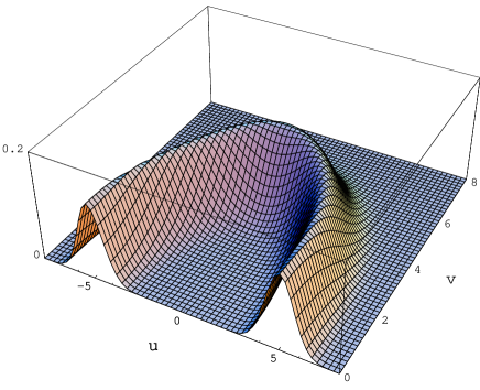
Figure 1: Left, the square of the wave packet $|\psi(u,v)|^{2}$ for $A^{*}(n)=\frac{\,\chi^{n}}{\,{\sqrt{2^{n}\,n!}}}e^{-\chi^{2}/4}$ and $\chi=5$. Right, the classical (dashed line) and bohmian (solid line) trajectories.

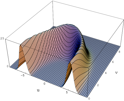
Figure 2: Left, the square of the wave packet $|\psi(u,v)|^{2}$ for $A^{*}(n)=\frac{n\,\chi^{n}}{\,{\sqrt{2^{n}\,n!}}}e^{-\chi^{2}/4}$ and $\chi=5$. Right, the classical (dashed line) and bohmian (solid line) trajectories.

4 Bohmian trajectories

To make the connection between the classical and quantum results more concrete, we can use the ontological interpretation of quantum mechanics [32, 33]. Moreover, since time is absent in quantum cosmology we can recover the notion of time using this formalism.

In ontological interpretation the wave function can be written as

$$\Psi(u,v)=R\,e^{iS}$$ (29)

where $R=R(u,v)$ and $S=S(u,v)$ are real functions and satisfy the following equations

$$-\frac{\partial^{2}R}{\partial u^{2}}+\frac{\partial^{2}R}{\partial v^{2}}+R\left(\frac{\partial S}{\partial u}\right)^{2}-R\left(\frac{\partial S}{\partial v}\right)^{2}+{\omega}^{2}(u^{2}-v^{2})R = 0,$$ (30)

$$R\frac{\partial^{2}S}{\partial u^{2}}-R\frac{\partial^{2}S}{\partial v^{2}}+2\frac{\partial R}{\partial u}\frac{\partial S}{\partial u}-2\frac{\partial R}{\partial v}\frac{\partial S}{\partial v} = 0.$$ (31)

To write $R$ and $S$, it is more appropriate to separate the real and imaginary parts of the wave packet

$$\Psi(u,v)=x(u,v)+iy(u,v)$$ (32)

where $x,y$ are real functions of $u$ and $v$. Using equation (29) we have

$$R = \sqrt{x^{2}+y^{2}}$$ (33)

$$S = \arctan\left(\frac{y}{x}\right)$$ (34)

On the other hand, the Bohmian trajectories, which determine the behavior of the scale factor, are governed by

$$p_{u}=\frac{\partial S}{\partial u},$$ (35)

$$p_{v}=\frac{\partial S}{\partial v}.$$ (36)

where the momenta correspond to the classical related Lagrangian ($L(q)=\dot{q}^{2}-V(q)$). Therefore, the equations of motion take the form

$$\dot{u}=\frac{1}{2}\frac{1}{1+\left(\frac{y}{x}\right)^{2}}\frac{d}{du}\left(\frac{y}{x}\right),$$ (37)

$$\dot{v}=-\frac{1}{2}\frac{1}{1+\left(\frac{y}{x}\right)^{2}}\frac{d}{dv}\left(\frac{y}{x}\right).$$ (38)

Using the explicit form of the wave packet (29), these differential equations can be solved numerically to find the time evolution of $u$ and $v$. In the right part of Figs. 1,2, we superimposed the classical and Bohmian trajectories for two different choices of initial conditions. The coincidence between these two trajectories is apparent from the figure. Moreover, the obtained Bohmian position versus time (i.e. $u(t)$) coincide well with its classical counterpart (Fig. 3). In particular, Fig. 4 shows the initial velocity at $v=0$ versus classical radius from classical and de-Brogli bohm points of view. As can be seen from the figure, the classical-quantum correspondence is manifest for large $\xi$, where $\xi$ is the classical radius of motion. In fact, the difference between classical and Bohmian results for small $\xi$ is due to the interference between the parts of the wave function and can be reduced by making the wave function more localized over the classical path [26].

Figure 3: Plot of $u(t)$ for Classical (dashed line) and Bohmian (solid line) trajectories where $A^{*}(n)=\frac{\chi^{n}}{\,{\sqrt{2^{n}\,n!}}}e^{-\chi^{2}/4}$ (left), $A^{*}(n)=\frac{n\,\chi^{n}}{\,{\sqrt{2^{n}\,n!}}}e^{-\chi^{2}/4}$ (right) and $\chi=5$.

Figure 4: Initial velocity ($\dot{v}(0)$) via classical (dashed line) and de-Brogli bohm interpretation of quantum mechanics (solid line).

5 Conclusions

We have studied $(n+1)$–dimensional cosmology with varying speed of light. We have obtained exact solutions in both classical and quantum levels for ($c\,$–$\Lambda$)–dominated Universe. We then constructed the wave packets via canonical proposal which exhibit a good classical-quantum correspondence. This method propose a particular relation between even and odd expansion coefficients which construct the initial wave functions and the initial derivative of the wave functions, respectively. In other words, canonical prescription define a particular connection between position and momentum distributions which at the same time correspond to their classical quantities and respect to the uncertainty relation. We have also studied the situation using de-Broglie Bohm interpretation of quantum mechanics. In fact, Bohmian trajectories highly depend on the wave function of the system and various linear combinations of eigenfunctions lead to different Bohmian trajectories. Therefore, the inconsistency between classical and Bohmian trajectories is natural in most cases. In this paper, using canonical prescription, we have tried to construct the wave packets which peak around the classical trajectories and simulate their classical counterparts. Using Bohmian interpretation we quantified our purpose of classical and quantum correspondence and showed that the Bohmian positions and momenta coincide well with their classical values upon choosing arbitrary but appropriate initial conditions. It is worth to mention that the classical and quantum correspondence issue has been attracted much attention in the literature [34]. In particular, Hawking and Page [35] and Kiefer [36] have also been studied the same WDW equation and discussed the situations where the resulting wave packets exhibit classical properties. But since the Kiefer’s proposal of initial condition result in the real wave function, it does not correspond to any classical trajectory. In summary, canonical proposal can be considered as a general, simple and efficient method to construct wave packets with a complete classical behavior for various physical models where we encounter with WDW-like equations.

References

- [1] J. Moffat, Int. J. of Physics D 2, 351 (1993); J. Moffat, Foundations of Physics, 23, 411 (1993).
- [2] A. Albrecht, J. Magueijo, Phys. Rev. D 59, 043516 (1999).
- [3] J. D. Barrow, Phys. Rev. D 59, 043515 (1999).
- [4] J. D. Barrow and J. Magueijo, Phys. Lett. B 443, 104 (1998).
- [5] J. D. Barrow and J. Magueijo, Phys. Lett. B 447, 246 (1999).
- [6] J. D. Barrow and J. Magueijo, Class. Quant. Grav. 16, 1435 (1999).
- [7] J. D. Barrow and J. Magueijo, Astrophys. J. Lett. 532, L87-90 (2000).
- [8] J. Moffat, astro-ph/9811390.
- [9] M. A. Clayton, J. W. Moffat, Phys. Lett. B 460, 263 (1999).
- [10] M. A. Clayton, J. W. Moffat, Phys. Lett. B 477, 269 (2000).
- [11] M. A. Clayton, J. W. Moffat, Int. J. Mod. Phys. D 11, 187 (2002).
- [12] I. Drummond, gr-qc/9908058.
- [13] P. P. Avelino and C. J. A. P. Martins, Phys.Lett. B 459, 468 (1999).
- [14] P. P. Avelino, C. J. A. P. Martins, and G. Rocha, Phys. Lett. B 483, 210 (2000).
- [15] T. Harko and M. K. Mak, Gen. Rel. Grav. 31, 849 (1999); Class. Quant. Grav. 16, 2741 (1999).
- [16] E. Kiritsis, JHEP 10, 010 (1999).
- [17] S. Alexander, JHEP 11, 017 (2000).
- [18] B. A. Bassett, S. Liberati, C. Molina-Paris, M. Visser, Phys. Rev. D 62, 103518 (2000).
- [19] J. Magueijo, Rep. Prog. Phys. 66, 2025 (2003).
- [20] G. F. R. Ellis, Gen. Relativ. Gravit. 39, 511 (2007).
- [21] J. Magueijo, J. W. Moffat, arXiv:0705.4507.
- [22] J. Magueijo, Phys. Rev. D 62, 103521 (2000).
- [23] T. Harko, H. Q. Lu, M. k. Mak and K. S. Cheng, Europhys. lett. 49, 814 (2000).
- [24] A. V. Yurov, V. A. Yurov, hep-th/0505034.
- [25] F. Shojai, S. Molladavoudi, Gen. Relativ. Gravit. 39, 795 (2007).
- [26] S. S. Gousheh, H. R. Sepangi, P. Pedram, and M. Mirzaei, Class. Quantum Grav. 24, 4377 (2007).
- [27] B. F. Schutz, Phys. Rev. D 2, 2762 (1970); B. F. Schutz, Phys. Rev. D 4, 3559 (1971).
- [28] P. Pedram, S. Jalalzadeh and S. S. Gousheh, Phys. Lett. B 655, 91 (2007), arXiv:0708.4143; P. Pedram, S. Jalalzadeh and S. S. Gousheh, Class. Quantum Grav. 24, 5515 (2007), arXiv:0709.1620; P. Pedram and S. Jalalzadeh, Phys. Lett. B (2007), doi:10.1016/j.physletb.2007.11.013, arXiv:0705.3587; P. Pedram, S. Jalalzadeh and S. S. Gousheh, Int. J. Theor. Phys. doi:10.1007/s10773-007-9436-9, arXiv:0705.3587; P. Pedram, M. Mirzaei, S. Jalalzadeh, and S. S. Gousheh, to appear in Gen. Relativ. Gravit.
- [29] J. Magueijo, Phys. Rev. D 63, 043502 (2001).
- [30] S. N. Manida, gr-qc/9905046.
- [31] S. S. Stepanov, physics/9909009, astro-ph/9909311.
- [32] P. R. Holland, The Quantum Theory of Motion: An Account of the de Broglie-Bohm Interpretation of Quantum Mechanics, Cambridge University Press, Cambridge (1993).
- [33] N. Pinto-Neto, Procedings of the VIII Brazilian School of Cosmology and Gravitation II, Edited by M. Novello (1999).
- [34] Quantum Cosmology and Baby Universe, Eds. S.Coleman, J.B.Hartle, T.Piran. and S.Weinberg, (World Scientific, 1991).
- [35] S. W. Hawking and Don N. Page, Phys. Rev. D 42, 2655 (1990).
- [36] Claus Kiefer, Phys. Rev. D 38, 1761 (1988); C. Kiefer, Quantum Gravity (Oxford University Press, Oxford, 2007), 2nd ed.