Maximum-Likelihood Priority-First Search Decodable Codes for Combined Channel Estimation and Error Protection

Abstract

The code that combines channel estimation and error protection has received general attention recently, and has been considered a promising methodology to compensate multi-path fading effect. It has been shown by simulations that such code design can considerably improve the system performance over the conventional design with separate channel estimation and error protection modules under the same code rate. Nevertheless, the major obstacle that prevents from the practice of the codes is that the existing codes are mostly searched by computers, and hence exhibit no good structure for efficient decoding. Hence, the time-consuming exhaustive search becomes the only decoding choice, and the decoding complexity increases dramatically with the codeword length. In this paper, by optimizing the signal-to-noise ratio, we found a systematic construction for the codes for combined channel estimation and error protection, and confirmed its equivalence in performance to the computer-searched codes by simulations. Moreover, the structural codes that we construct by rules can now be maximum-likelihoodly decodable in terms of a newly derived recursive metric for use of the priority-first search decoding algorithm. Thus, the decoding complexity reduces significantly when compared with that of the exhaustive decoder. The extension code design for fast-fading channels is also presented. Simulations conclude that our constructed extension code is robust in performance even if the coherent period is shorter than the codeword length.

I Introduction

The new demand of wireless communications in recent years inspires a quick advance in wireless transmission technology. Technology blossoms in both high-mobility low-bit-rate and low-mobility high-bit-rate transmissions. Apparently, the next challenge in wireless communications would be to reach high transmission rate under high mobility. The main technology obstacle for high-bit-rate transmission under high mobility is the seemingly highly time-varying channel characteristic due to movement; such a characteristic further enforces the difficulty in compensating the intersymbol interference. Presently, a typical receiver for wireless communications usually contains separate modules respectively for channel estimation and channel equalization. The former module estimates the channel parameters based on a known training sequence or pilots, while the latter module uses these estimated channel parameters to eliminate the channel effects due to multipath fading. However, the effectiveness in channel fading elimination for such a system structure may be degraded at a fast time-varying environment, which makes high-bit-rate transmission under high-mobility environment a big challenge.

Recent researches [3][6][11][17][18] have confirmed that better system performance can be obtained by jointly considering a number of system devices, such as channel coding, channel equalization, channel estimation, and modulation, when compared with the system with individually optimized devices. Specially, some works on combining devices of codeword decision and channel effect cancellation in typical receivers can appropriately exclude channel estimation labor and still perform well. In 1994, Seshadri [17] first proposed a blind maximum-likelihood sequence estimator (MLSE) in which the data and channel are simultaneously estimated. Skoglund et al [18] later provided a milestone evidence for the fact that the joint design system is superior in combating with serious multipath block fading. They also applied similar technique to a multiple-input-multiple-output (MIMO) system at a subsequent work [6]. In short, Skoglund et al looked for the non-linear codes that are suitable for this channel by computer search. Through simulations, they found that the non-linear code that combines channel estimation and error protection, when being carefully designed by considering multipath fading effect, outperforms a typical communication system with perfect channel estimation by at least 2 dB. Their results suggest the high potential of applying a single, perhaps non-linear, code to improve the transmission rate at a highly mobile environment, at which channel estimation becomes technically infeasible. Similar approach was also proposed by [3], and the authors actually named such codes the training codes. In [2], Chugg and Polydoros derived a recursive metric for joint maximum-likelihood (ML) decoding, and hint that the recursive metric may only be used with the sequential algorithms [1]. As there are no efficient decoding approaches for the codes mentioned above, these authors mostly considered only codes of short length, or even just the principle of code design for combined channel estimation and error protection.

One of the drawbacks of these combined-channel-estimation-and-error-protection codes is that only exhaustive search can be used to decode their codewords due to lack of systematic structure. Such drawback apparently inhibits the use of the codes for combined channel estimation and error protection in practical applications. This leads to a natural research query on how to construct an efficiently decodable code with channel estimation and error protection functions.

In this work, the research query was resolved by first finding that the codeword that maximizes the system signal-to-noise ratio (SNR) should be orthogonal to its delayed counterpart. We then found that the code consists of the properly chosen self-orthogonal codewords can compete with the computer-searched codes in performance. With this self-orthogonality property, the maximum-likelihood metrics for these structural codewords can be equivalently fit into a recursive formula, and hence, the priority-first search decoding algorithm can be employed. As a consequence, the decoding complexity, as compared to the exhaustive decoding, reduces considerably. Extensions of our proposed coding structure that was originally designed for channels with constant coefficients to channels with varying channel coefficients within a codeword block are also established. Simulations conclude that our constructed extension code is robust even for a channel whose coefficients vary more often than a coding block.

The paper is organized as follows. Section II describes the system model considered, followed by the technical backgrounds required in this work. In Section III, the coding rule that optimizes the system SNR is established, and is subsequently used to construct the codes for combined channel estimation and error protection. The corresponding recursive maximum-likelihood decoding metrics for our rule-based systematic codes are derived in Section IV. Simulations are summarized and remarked in Section V. Extension to channels with varying coefficients within a codeword is presented in Section VI. Section VII concludes the paper.

In this work, superscripts “$H$” and “$T$” specifically reserve for the representations of matrix Hermitian transpose and transpose operations, respectively [10], and should not be confused with the matrix exponent.

II Background

II-A System model and maximum-likelihood decoding criterion

The system model defined in this section and the notations used throughout follow those in [18].

Transmit a codeword $\boldsymbol{b}=[\begin{matrix}b_{1},\cdots,b_{N}\end{matrix}]^{T}$, where each $b_{j}\in\{\pm 1\}$, of a $(N,K)$ code ${\mathcal{C}}$ over a block fading (specifically, quasi-static fading) channel of memory order $(P-1)$. Denote the channel coefficients by $\boldsymbol{h}=[\begin{matrix}h_{1},\cdots h_{P}\end{matrix}]^{T}$ that are assumed constant within a coding block. The complex-valued received vector is then given by:

$$\boldsymbol{y}=\mathbb{B}\boldsymbol{h}+\boldsymbol{n},$$ (1)

where $\boldsymbol{n}$ is zero-mean complex-Gaussian distributed with $E[\boldsymbol{n}\boldsymbol{n}^{H}]=\sigma_{n}^{2}\mathbb{I}_{L}$, $\mathbb{I}_{L}$ is the $L\times L$ identity matrix, and

$$\mathbb{B}\triangleq\begin{bmatrix}b_{1}&0&\cdots&0\\ \vdots&b_{1}&\ddots&\vdots\\ b_{N}&\vdots&\ddots&0\\ 0&b_{N}&\ddots&b_{1}\\ \vdots&\ddots&\ddots&\vdots\\ 0&0&\cdots&b_{N}\end{bmatrix}_{L\times P}.$$

Some assumptions are made in the following. Both the transmitter and the receiver know nothing about the channel coefficients $\boldsymbol{h}$, but have the knowledge of multipath parameter $P$ or its upper bound. Besides, there are adequate guard period between two encoding blocks so that zero interblock interference is guaranteed. Based on the system model in (1) and the above assumptions, we can derive [18] the least square (LS) estimate of channel coefficients $\boldsymbol{h}$ for a given $\boldsymbol{b}$ (interchangeably, $\mathbb{B}$) as:

$$\hat{\boldsymbol{h}}=(\mathbb{B}^{T}\mathbb{B})^{-1}\mathbb{B}^{T}\boldsymbol{y},$$

and the joint maximum-likelihood (ML) decision on the transmitted codeword becomes:

$$\hat{\boldsymbol{b}}=\arg\min_{\boldsymbol{b}\in{{\mathcal{C}}}}\|\boldsymbol{y}-\mathbb{B}\hat{\boldsymbol{h}}\|^{2}=\arg\min_{\boldsymbol{b}\in{{\mathcal{C}}}}\|\boldsymbol{y}-\mathbb{P}_{B}\boldsymbol{y}\|^{2},$$ (2)

where $\mathbb{P}_{B}=\mathbb{B}(\mathbb{B}^{T}\mathbb{B})^{-1}\mathbb{B}^{T}$. Notably, codeword $\boldsymbol{b}$ and transformed codeword $\mathbb{P}_{B}$ is not one-to-one corresponding unless the first element of $\boldsymbol{b}$, namely $b_{1}$, is fixed. For convenience, we will always set $b_{1}=-1$ for the codebooks we construct in the sequel.

II-B Summary of previous and our code designs for combined channel estimation and error protection

In literatures, no systematic code constructions have been proposed for combined channel estimation and error protection for quasi-static fading channels. Efforts were mostly placed on how to find the proper sequences to compensate the channel fading by computer searches [3][6][13][14][18][19][21]. Decodability for the perhaps structureless computer-searched codes thus becomes an engineering challenge.

In 2003, Skoglund, Giese and Parkvall [18] searched by computers for nonlinear binary block codes suitable for combined estimation and error protection for quasi-static fading channels by minimizing the sum of the pairwise error probabilities (PEP) under equal prior, namely,

$$P_{e}\leq\frac{1}{2^{K}}\sum_{i=1}^{2^{K}}\sum_{j=1,j\neq i}^{2^{K}}\Pr\left(\left.\hat{\boldsymbol{b}}=\boldsymbol{b}(j)\right|\boldsymbol{b}(i)\mbox{ transmitted}\right),$$ (3)

where $\boldsymbol{b}(i)$ denotes the $i$th codeword of the $(N,K)$ nonlinear block code. Although the operating signal-to-noise ratio (SNR) for the code search was set at $10$ dB, their simulation results showed that the found codes perform well in a wide range of different SNRs. In addition, the mismatch in the relative powers of different channel coefficients, as well as in the channel Rice factors [20], has little effect on the resultant performance. It was concluded that in comparison with the system with the benchmark error correcting code and the perfect channel estimator, significant performance improvement can be obtained by adopting their computer-searched nonlinear codes.

Later in 2005, Coskun and Chugg [3] replaced the PEP in (3) by a properly defined pairwise distance measure between two codewords, and proposed a suboptimal greedy algorithm to speed up the code search process. In 2007, Giese and Skoglund [6] re-applied their original idea to the single- and multiple-antenna systems, and used the asymptotic PEP and the generic gradient-search algorithm in place of the PEP and the simulated annealing algorithm in [18] to reduce the system complexity.

At the end of [18], the authors pointed out that “an important topic for further research is to study how the decoding complexity of the proposed scheme can be decreased.” They proceeded to state that along this research line, “one main issue is to investigate what kind of structure should be enforced on the code to allow for simplified decoding.”

Stimulating from these ending statements, we take a different approach for code design. Specifically, we pursued and established a systematic code design rule for combined channel estimation and error protection for quasi-static fading channels, and confirmed that the codes constructed based on such rule maximize the average system SNR. As so happened that the computer-searched code in [18] satisfies such rule, its insensitivity to SNRs, as well as channel mismatch, somehow finds the theoretical footing. Enforced by the systematic structure of our rule-based constructed codes, we can then derive a recursive maximum-likelihood decoding metric for use of priority-first search decoding algorithm. The decoding complexity is therefore significantly decreased at moderate-to-high SNRs as contrary to the obliged exhaustive decoder for the structureless computer-searched codes.

It is worth mentioning that although the codes searched by computers in [6][18] target the unknown channels, for which the channel coefficients are assumed constant in a coding block, the evaluation of the PEP criterion does require to presume the knowledge of channel statistics. The code constructed based on the rule we proposed, however, is guaranteed to maximize the system SNR regardless of the statistics of the channels. This hints that our code can still be well applied to the situation where channel blindness becomes a strict system restriction. Details will be introduced in subsequent sections.

II-C Maximum-likelihood priority-first search decoding algorithm

For a better understanding, we give a short description of a code tree for the $(N,K)$ code $\mathcal{C}$ over which the decoding search is performed before our describing the priority-first search decoding algorithm in this subsection.

A code tree of a $(N,K)$ binary code represents every codeword as a path on a binary tree as shown in Fig. 1. The code tree consists of $(N+1)$ levels. The single leftmost node at level zero is usually called the origin node. There are at most two branches leaving each node at each level. The $2^{K}$ rightmost nodes at level $N$ are called the terminal nodes.

Each branch on the code tree is labeled with the appropriate code bit $b_{i}$. As a convention, the path from the single origin node to one of the $2^{K}$ terminal nodes is termed the code path corresponding to the codeword. Since there is a one-to-one correspondence between the codeword and the code path of $\mathcal{C}$, a codeword can be interchangeably referred to by its respective code path or the branch labels that the code path traverses. Similarly, for any node in the code tree, there exists a unique path traversing from the single original node to it; hence, a node can also be interchangeably indicated by the path (or the path labels) ending at it. We can then denote the path ending at a node at level $\ell$ by the branch labels $[b_{1},b_{2},\cdots,b_{\ell}]$ it traverses. For convenience, we abbreviates $[b_{1},b_{2},\cdots,b_{\ell}]^{T}$ as $\boldsymbol{b}_{(\ell)}$, and will drop the subscript when $\ell=N$. The successor pathes of a path $\boldsymbol{b}_{(\ell)}$ are those whose first $\ell$ labels are exactly the same as $\boldsymbol{b}_{(\ell)}$.

Figure 1: The code tree for a computer-searched PEP-minimum $(4,2)$ code with $b_{1}$ fixed as $-1$.

The priority-first search on a code tree is guided by an evaluation function $f$ that is defined for every path. It can be typically algorithmized as follows.

• (Initialization) Load the Stack with the path that ends at the original node.

• (Evaluation) Evaluate the $f$-function values of the successor paths of the current top path in the Stack, and delete this top path from the Stack.

• (Sorting) Insert the successor paths obtained in Step 2 into the Stack such that the paths in the Stack are ordered according to ascending $f$-function values of them.

• (Loop) If the top path in the Stack ends at a terminal node in the code tree, output the labels corresponding to the top path, and the algorithm stops; otherwise, go to Step 2.

It remains to find the evaluation function $f$ that secures the maximum-likelihoodness of the output codeword. We begin with the introduction of a sufficient condition under which the above priority-first search algorithm guarantees to locate the code path with the smallest $f$-function value among all code paths of ${\mathcal{C}}$.

Lemma 1

If $f$ is non-decreasing along every path $\boldsymbol{b}_{(\ell)}$ in the code tree, i.e.,

$$f\left(\boldsymbol{b}_{(\ell)}\right)\leq\min_{\left\{\tilde{\boldsymbol{b}}\in{\mathcal{C}}~{}:~{}\tilde{\boldsymbol{b}}_{(\ell)}=\boldsymbol{b}_{(\ell)}\right\}}f(\tilde{\boldsymbol{b}}),$$ (4)

the priority-first search algorithm always outputs the code path with the smallest $f$-function value among all code paths of ${\mathcal{C}}$.

Proof:

Let $\boldsymbol{b}^{\ast}$ be the first top path that reaches a terminal node (and hence, is the output code path of the priority-first search algorithm.) Then, Step 3 of the algorithm ensures that $f\left(\boldsymbol{b}^{\ast}\right)$ is no larger than the $f$-function value of any path currently in the Stack. Since condition (4) guarantees that the $f$-function value of any other code path, which should be the offspring of some path $\boldsymbol{b}_{(\ell)}$ existing in the Stack, is no less than $f\left(\boldsymbol{b}_{(\ell)}\right)$, we have

$$f\left(\boldsymbol{b}^{\ast}\right)\leq f\left(\boldsymbol{b}_{(\ell)}\right)\leq\min_{\left\{\tilde{\boldsymbol{b}}\in{\mathcal{C}}~{}:~{}\tilde{\boldsymbol{b}}_{(\ell)}=\boldsymbol{b}_{(\ell)}\right\}}f(\tilde{\boldsymbol{b}}).$$

Consequently, the lemma follows. ∎

In the design of the search-guiding function $f$, it is convenient to divide it into the sum of two parts. In order to perform maximum-likelihood decoding, the first part $g$ can be directly defined based on the maximum-likelihood metric of the codewords such that from (2),

$$\arg\min_{\boldsymbol{b}\in{\mathcal{C}}}g(\boldsymbol{b})=\arg\min_{\boldsymbol{b}\in{{\mathcal{C}}}}\|\boldsymbol{y}-\mathbb{P}_{B}\boldsymbol{y}\|^{2}.$$

After $g$ is defined, the second part $h$ can be designed to validate (4) with $h(\boldsymbol{b})=0$ for any $\boldsymbol{b}\in{\mathcal{C}}$. Then, from $f(\boldsymbol{b})=g(\boldsymbol{b})+h(\boldsymbol{b})=g(\boldsymbol{b})$ for all $\boldsymbol{b}\in{\mathcal{C}}$, the desired maximum-likelihood priority-first search decoding algorithm is established since (4) is valid.

In principle, both $g(\cdot)$ and $h(\cdot)$ range over all possible paths in the code tree. The first part, $g(\cdot)$, is simply a function of all the branches traversed thus far by the path, while the second part, $h(\cdot)$, called the heuristic function, helps predicting a future route from the end node of the current path to a terminal node [8]. Notably, the design of the heuristic function $h$ that makes valid condition (4) is not unique. Different designs may result in variations in computational complexity.

We close this section by summarizing the target of this work based on what have been mentioned in this section.

1. A code of comparable performance to the computer-searched code is constructed according to certain rules so that its code tree can be efficiently and systematically generated (Section III).

2. Efficient recursive computation of the maximum-likelihood evaluation function $f$ from the predecessor path to the successor paths is established (Section IV).

3. With the availability of items 1 and 2, the construction and maximum-likelihood decoding of codes with longer codeword length becomes possible, and hence, makes the assumption that the unknown channel coefficients $\boldsymbol{h}$ are fixed during a long coding block somewhat impractical especially for mobile transceivers. Extension of items 1 and 2 to the unknown channels whose channel coefficients may change several times during one coding block will be further proposed (Section VI).

III Code Construction

In this section, the code design rule that guarantees the maximization of the system SNR regardless of the channel statistics is presented, followed by the algorithm to generate the code based on such rule.

III-A Code rule that maximizes the average SNR

A known inequality [15] for the multiplication of two positive semidefinite Hermitian matrices, $\mathbb{A}$ and $\mathbb{B}$, is that

$$\mathrm{tr}(\mathbb{A}\mathbb{B})\leq\mathrm{tr}(\mathbb{A})\cdot\lambda_{\max}(\mathbb{B}),$$ (5)

where $\mathrm{tr}(\cdot)$ represents the matrix trace operation, and $\lambda_{\max}(\mathbb{B})$ is the maximal eigenvalue of $\mathbb{B}$ [10]. The above inequality holds with equality when $\mathbb{B}$ is an identity matrix.

From the system model $\boldsymbol{y}=\mathbb{B}\boldsymbol{h}+\boldsymbol{n}$, it can be derived that the average SNR satisfies:

Average SNR $$= \frac{E[\|\mathbb{B}\boldsymbol{h}\|^{2}]}{E[\|\boldsymbol{n}\|^{2}]}$$

$$= \frac{E[\mathrm{tr}(\boldsymbol{h}^{H}\mathbb{B}^{T}\mathbb{B}\boldsymbol{h})]}{L\sigma_{n}^{2}}$$

$$= \frac{\mathrm{tr}(E[\boldsymbol{h}\boldsymbol{h}^{H}]\mathbb{B}^{T}\mathbb{B})}{L\sigma_{n}^{2}}$$

$$= \frac{N}{L}\frac{1}{\sigma_{n}^{2}}\mathrm{tr}\left(E[\boldsymbol{h}\boldsymbol{h}^{H}]\frac{1}{N}\mathbb{B}^{T}\mathbb{B}\right)$$

$$\leq \frac{N}{L}\frac{1}{\sigma_{n}^{2}}\mathrm{tr}(E[\boldsymbol{h}\boldsymbol{h}^{H}])\lambda_{\max}\left(\frac{1}{N}\mathbb{B}^{T}\mathbb{B}\right).$$

Then, the theories on Ineq. (5) result that taking

$$\frac{1}{N}\mathbb{B}^{T}\mathbb{B}=\mathbb{I}_{P}\triangleq\begin{bmatrix}1&0&\cdots&0\\ 0&1&\cdots&0\\ \vdots&\vdots&\ddots&\vdots\\ 0&0&\cdots&1\end{bmatrix}_{P\times P}$$ (6)

will optimize the average SNR regardless of the statistics of $\boldsymbol{h}$ [5].

Existence of codeword sequences satisfying (6) is promised only for $P=2$ with $N$ odd (and trivially, $P=1$). In some other cases such as $P=3$, one can only design codes to approximately satisfy (6) as:

$$\frac{1}{N}\mathbb{B}^{T}\mathbb{B}=\begin{bmatrix}1&\pm\displaystyle\frac{1}{N}&0\\ \pm\displaystyle\frac{1}{N}&1&\pm\displaystyle\frac{1}{N}\\ 0&\pm\displaystyle\frac{1}{N}&1\end{bmatrix}\mbox{ for }N\mbox{ even,}$$

and

$$\frac{1}{N}\mathbb{B}^{T}\mathbb{B}=\begin{bmatrix}1&0&\pm\displaystyle\frac{1}{N}\\ 0&1&0\\ \pm\displaystyle\frac{1}{N}&0&1\end{bmatrix}\mbox{ for }N\mbox{ odd}.$$

Owing to this observation, we will relax (6) to allow some off-diagonal entries in $\mathbb{B}^{T}\mathbb{B}$ to be either $1$ or $-1$ whenever a strict maintenance of (6) is impossible.

Empirical examination by simulated-annealing code-search algorithm shows that for $4\leq N\leq 16$ and $N$ even, the best half-rate codes that minimize the sum of PEPs in (3) under complex zero-mean Gaussian distributed $\boldsymbol{h}$ with $E[\boldsymbol{h}\boldsymbol{h}^{H}]=(1/2)\mathbb{I}_{P}$ and $P=2$ all satisfy that

$$\mathbb{B}^{T}\mathbb{B}=\begin{bmatrix}N&\pm 1\\ \pm 1&N\end{bmatrix}$$ (7)

except three codewords at $N=14$. A possible cause for the appearance of three exception codewords at $N=14$ is that the best code that minimizes the sum of the pairwise error probabilities may not be the truly optimal code that reaches the smallest error probability, and hence, does not necessarily yield the maximum average SNR as demanded by (6). We have also obtained and examined the computer-searched code used in [18] for $N=22$, and found as anticipated that every codeword carries the property of (7).

The operational meaning of the condition $\mathbb{B}^{T}\mathbb{B}=N\cdot\mathbb{I}_{P}$ is that the codeword is orthogonal to its shifted counterpart, and hence, a space-diversity nature is implicitly enforced. This coincides with the conclusion made in [4] that the training sequence satisfying that $\mathbb{B}^{T}\mathbb{B}$ is proportional to $\mathbb{I}_{P}$ can provide optimal channel estimation performance. It should be mentioned that codeword condition (6) has been identified in [6], and the authors in [6, pp. 1591] remarked that a code sequence with certain aperiodic autocorrelation property can possibly be exploited in future code design approaches, which is one of the main research goals of this paper.

III-B Equivalent system model for combined channel estimation and error protection codes

Figure 2: Equivalent system model for combined channel estimation and error protection codes.

By noting that $\mathbb{P}_{B}$ is idempotent and symmetric, and both $\mathrm{tr}(\mathbb{P}_{B})$ and $\|\mathrm{vec}(\mathbb{P}_{B})\|^{2}$ are equal to $P$, where $\mathrm{vec}(\cdot)$ denotes the operation to transform an $(M\times N)$ matrix into a $(MN\times 1)$ vector, the best joint maximum-likelihood decision in (2) can be reformulated as:

$$\hat{\boldsymbol{b}} = \arg\min_{\boldsymbol{b}\in{\mathcal{C}}}\|\boldsymbol{y}-\mathbb{P}_{B}\boldsymbol{y}\|^{2}$$

$$= \arg\min_{\boldsymbol{b}\in{\mathcal{C}}}(\boldsymbol{y}-\mathbb{P}_{B}\boldsymbol{y})^{H}(\boldsymbol{y}-\mathbb{P}_{B}\boldsymbol{y})$$

$$= \arg\min_{\boldsymbol{b}\in{\mathcal{C}}}(\boldsymbol{y}^{H}\boldsymbol{y}-\boldsymbol{y}^{H}\mathbb{P}_{B}\boldsymbol{y})$$

$$= \arg\min_{\boldsymbol{b}\in{\mathcal{C}}}-\mathrm{tr}(\mathbb{P}_{B}\boldsymbol{y}\boldsymbol{y}^{H})$$

$$= \arg\min_{\boldsymbol{b}\in{\mathcal{C}}}\left(\|\mathrm{vec}(\boldsymbol{y}\boldsymbol{y}^{H})\|^{2}-\mathrm{vec}(\mathbb{P}_{B})^{T}\mathrm{vec}(\boldsymbol{y}\boldsymbol{y}^{H})-\mathrm{vec}(\boldsymbol{y}\boldsymbol{y}^{H})^{H}\mathrm{vec}(\mathbb{P}_{B})+\|\mathrm{vec}(\mathbb{P}_{B})\|^{2}\right)$$

$$= \arg\min_{\boldsymbol{b}\in{\mathcal{C}}}\|\mathrm{vec}(\boldsymbol{y}\boldsymbol{y}^{H})-\mathrm{vec}(\mathbb{P}_{B})\|^{2}.$$ (9)

We therefore transform the original system in (1) to an equivalent system model that contains an outer product demodulator and a minimum Euclidean distance selector at the $\mathbb{P}_{B}$-domain as shown in Fig. 2. As the outer product demodulator can be viewed as a generalization of the square-law combining that is of popular use in non-coherent detection for both slow and fast fading [16], the above equivalent transformation suggests a potential application of combined channel estimate and error protection codes for the non-coherent system in which the fading is rapid enough to preclude a good estimate of the channel coefficients. Further discussion on how to design codes for unknown fast-fading channels will be continued in Section VI.

As a consequence of (9), the maximum-likelihood decoding is to find the codeword $\mathbb{P}_{B}$ whose Euclidean distance to $\boldsymbol{y}\boldsymbol{y}^{H}$ is the smallest. Similar to (3), we can then bound the error probability by:

$$\!\!\!\!\!\!\!\!\!P_{e}\leq\frac{1}{2^{K}}\sum_{i=1}^{2^{K}}\sum_{j=1\atop j\neq i}^{2^{K}}\Pr\!\left(\left.\|\mathrm{vec}(\boldsymbol{y}\boldsymbol{y}^{H})-\mathrm{vec}(\mathbb{P}_{B(j)})\|^{2}\!<\!\|\mathrm{vec}(\boldsymbol{y}\boldsymbol{y}^{H})-\mathrm{vec}(\mathbb{P}_{B(i)})\|^{2}\right|\boldsymbol{b}(i)\mbox{ transmitted}\right).$$

(10)

The PEP-based upper bound in (10) hints that a good code design should have an adequately large pairwise Euclidean distance

$$\|\mathrm{vec}(\mathbb{P}_{B(i)})-\mathrm{vec}(\mathbb{P}_{B(j)})\|^{2}$$ (11)

among all codeword pairs $\mathbb{P}_{B(i)}$ and $\mathbb{P}_{B(j)}$, where $\mathbb{P}_{B(i)}$ is the equivalent codeword at the $\mathbb{P}_{B}$-domain, and is one-to-one corresponding to the codeword $\boldsymbol{b}(i)$ if $b_{1}$ is fixed and known. Based on this observation, we may infer under equal prior that a uniform draw of codewords satisfying $\mathbb{B}^{T}\mathbb{B}=N\cdot\mathbb{I}_{P}$ at the $\mathbb{P}_{B}$-domain may asymptotically result in a good code. In light of the one-to-one correspondence relation between $\boldsymbol{b}$ and $\mathbb{P}_{B}$, we may further infer that uniform selection of codewords in the set of

$${\mathcal{A}}\triangleq\left\{\mathbb{P}_{B}=\mathbb{B}(\mathbb{B}^{T}\mathbb{B})^{-1}\mathbb{B}~{}:~{}\exists\boldsymbol{b}\in\{\pm 1\}^{N}\mbox{ such that }\mathbb{B}^{T}\mathbb{B}=N\cdot\mathbb{I}_{P}\right\}$$

is conceptually equivalent to uniform-pick of codewords in $\{\boldsymbol{b}\in\{\pm 1\}^{N}:\mathbb{B}^{T}\mathbb{B}=N\mathbb{I}_{P}\}$.

Recall that in order to perform the priority-first search decoding on a code tree, an efficient and systematic way to generate the code tree (or more specifically, an efficient and systematic way to generate the successor paths of the top path) is necessary. The uniform pick principle then suggests that considering only the codewords with the same prefix $[b_{1},\cdots,b_{\ell}]$, the ratio of the number of codewords satisfying $b_{\ell+1}=-1$ with respect to the candidate sequence pool shall be made equal to that of codewords satisfying $b_{\ell+1}=1$, whenever possible. This can be mathematical interpreted as:

$$\frac{|{\mathcal{C}}(b_{1},b_{2},\cdots,b_{\ell},+1)|}{\left|{\mathcal{A}}(b_{1},b_{2},\cdots,b_{\ell},+1|N\cdot\mathbb{I}_{P})\right|}\approx\frac{|{\mathcal{C}}(b_{1},b_{2},\cdots,b_{\ell},-1)|}{\left|{\mathcal{A}}(b_{1},b_{2},\cdots,b_{\ell},-1|N\cdot\mathbb{I}_{P})\right|},$$ (12)

where ${\mathcal{C}}(\boldsymbol{b}_{(\ell)})$ is the set of all codewords whose first $\ell$ bits equal $b_{1},b_{2},\cdots,b_{\ell}$, and ${\mathcal{A}}(\boldsymbol{b}_{(\ell)}|\mathbb{G})$ is the set of all possible $\pm 1$-sequences of length $N$, whose first $\ell$ bits equal $b_{1},b_{2},\cdots,b_{\ell}$ and whose $\mathbb{B}$-representation satisfies $\mathbb{B}^{T}\mathbb{B}=\mathbb{G}$. Accordingly, if $|{\mathcal{A}}(\boldsymbol{b}_{(\ell)}|\mathbb{G})|$ can be computed explicitly, the desired efficient and systematic generation of the code tree becomes straightforward.

Simulations on the above uniform selective code over $\{\boldsymbol{b}\in\{\pm 1\}^{N}:\mathbb{B}^{T}\mathbb{B}=N\mathbb{I}_{P}\}$ show that its performance is almost the same as the computer-searched code that minimizes the sum of PEPs. Hence, the maximizing-the-pairwise-Euclidean-distance intuition we adopt for code design performs well as we have anticipated.

In the next subsection, we will provide an exemplified encoding algorithm based on the above basic rule specifically for channels of memory order $1$, namely, $P=2$. The encoding algorithm for larger memory order can be similarly built.

III-C Exemplified encoding algorithm for channels of memory order one

Before the presentation of the exemplified encoding algorithm, the explicit formula for $|{\mathcal{A}}(\boldsymbol{b}_{(\ell)}|\mathbb{G})|$ needs to be established first.

Lemma 2

Fix $P=2$. Then, for $N$ odd, and $\mathbb{G}=N\cdot\mathbb{I}_{P}$,

$$|{\mathcal{A}}(\boldsymbol{b}_{(\ell)}|\mathbb{G})|=\displaystyle\binom{N-\ell}{(N-\ell-m_{\ell})/2}{\bf 1}\left\{\left|m_{\ell}\right|\leq N-\ell\right\}\mbox{ for }1\leq\ell\leq N,$$

where ${\bf 1}\{\cdot\}$ is the set indicator function, and $m_{\ell}\triangleq(b_{1}b_{2}+\cdots+b_{\ell-1}b_{\ell})\cdot{\bf 1}\{\ell>1\}$.

In addition, for $N$ even, and

$$\mathbb{G}_{1}\triangleq\begin{bmatrix}N&-1\\ -1&N\end{bmatrix}\quad\mbox{and}\quad\mathbb{G}_{2}\triangleq\begin{bmatrix}N&1\\ 1&N\end{bmatrix},$$

$$|{\mathcal{A}}(\boldsymbol{b}_{(\ell)}|\mathbb{G}_{\theta})|=\displaystyle\binom{N-\ell}{(N-\ell+(-1)^{\theta}-m_{\ell})/2}{\bf 1}\left\{\left|(-1)^{\theta}-m_{\ell}\right|\leq N-\ell\right\}\mbox{ for }1\leq\ell\leq N.$$

Here, we assume that $\binom{0}{0}=1$ specifically for the case of $\ell=N$.

Proof:

The lemma requires

$$c=b_{1}b_{2}+b_{2}b_{3}+\cdots+b_{N-1}b_{N}=m_{\ell}+b_{\ell}b_{\ell+1}+\cdots+b_{N-1}b_{N},$$ (13)

where $c=0,-1,+1$ respectively for $\mathbb{G}$, $\mathbb{G}_{1}$ and $\mathbb{G}_{2}$. In order to satisfy (13), there should be $(N-\ell+c-m_{\ell})/2$ of $\{b_{\ell}b_{\ell+1},b_{\ell+1}b_{\ell+2},\cdots,b_{N-1}b_{N}\}$ equal to $1$, and the remaining of them equal $-1$, provided that $(N-\ell+c-m_{\ell})/2\geq 0$ and $(N-\ell)-(N-\ell+c-m_{\ell})/2\geq 0$. Notably, $(N-\ell+c-m_{\ell})$ is always an even number for the cases considered in the lemma. The proof is then completed by the observation that $[b_{\ell}b_{\ell+1},b_{\ell+1}b_{\ell+2},\cdots,b_{N-1}b_{N}]$ and $[b_{\ell+1},b_{\ell+2},\cdots,b_{N}]$ are one-to-one correspondence for given $b_{\ell}$. ∎

It is already hint in the above lemma that for $N$ odd, our encoding algorithm will uniformly pick $2^{K}$ codewords from the candidate sequences satisfying the exact SNR-maximization condition $\mathbb{B}^{T}\mathbb{B}=N\cdot\mathbb{I}_{P}$. However, for $N$ even, two conditions on candidate sequences will be used. Half of the codewords will be uniformly drawn from those candidate sequences satisfying $\mathbb{B}^{T}\mathbb{B}=\mathbb{G}_{1}$, and the other half of the codewords agree with $\mathbb{B}^{T}\mathbb{B}=\mathbb{G}_{2}$. The proposed codeword selection process is simply to list all the candidate sequences in binary-alphabetical order, starting from zero, and uniformly pick the codewords from the ordered list in every $\Delta$ interval, where

$$\Delta=\left\lfloor\frac{|{\mathcal{A}}(b_{1}=-1|\mathbb{H})|-1}{2^{K}/\Theta-1}\right\rfloor,$$

where $\mathbb{H}$ represents the desired $\mathbb{B}^{T}\mathbb{B}$, and $\Theta$ is the number of conditions and equals $1$ for $N$ odd, and $2$ for $N$ even. As a result, the selected codewords are those sequences with index $i\times\Delta$ for integer $i$. The encoding algorithm is summarized in the following.

• (Input) Let $i$ be the index of the requested codeword in the desired $(N,K)$ block code, where $0\leq i\leq 2^{K}-1$.

• (Initialization) Set $\Theta=1$ for $N$ odd, and $2$ for $N$ even. Let $b_{1}=-1$. Put (in terms of the notations in Lemma 2):

  $$\mathbb{H}=\left\{\begin{array}[]{ll}\mathbb{G},&\mbox{if }N\mbox{ odd};\\ \mathbb{G}_{1},&\mbox{if }N\mbox{ even and }0\leq i<2^{K-1};\\ \mathbb{G}_{2},&\mbox{if }N\mbox{ even and }2^{K-1}\leq i<2^{K}.\end{array}\right.$$

  Compute

  $$\Delta=\left\lfloor\frac{|{\mathcal{A}}(b_{1}|\mathbb{H})|-1}{2^{K}/\Theta-1}\right\rfloor.$$

  Also, re-adjust $i=i-2^{K-1}$ if $N$ is even and $2^{K-1}\leq i<2^{K}$.

  Let the minimum candidate sequence index $\rho_{\min}$ and the maximum candidate sequence index $\rho_{\max}$ in ${\mathcal{A}}(b_{1}|\mathbb{H})$ be respectively

  $$\rho_{\min}=0\quad{\rm and}\quad\rho_{\max}=|{\mathcal{A}}(b_{1}|\mathbb{H})|-1.$$

  Initialize $\ell=1$ and $\rho=i\times\Delta$.

• (Generation of the next code bit)

  Set $\ell=\ell+1$, and compute $\gamma=|{\mathcal{A}}(\boldsymbol{b}_{(\ell-1)},-1|\mathbb{H})|$.

  If $\rho<\rho_{\min}+\gamma$, then the next code bit $b_{\ell}=-1$, and re-adjust $\rho_{\max}=\rho_{\min}+\gamma-1$;

  else, the next code bit $b_{\ell}=1$, and re-adjust $\rho_{\min}=\rho_{\min}+\gamma$.

• (Loop) If $\ell=N$, output codeword $\boldsymbol{b}$, and the algorithm stops; otherwise, go to Step 3.

IV Maximum-Likelihood Priority-First Search Decoding of Combined Channel Estimation and Error Protection Codes

In this section, a recursive maximum-likelihood metric $g$ and its heuristic function $h$ for use of the priority-first search decoding algorithm to decode the structural codewords over multiple code trees are established.

IV-A Recursive maximum-likelihood metric $g$ for priority-first search over multiple code trees

Let ${\mathcal{C}}_{\theta}$ be the set of the codewords that satisfy $\mathbb{B}^{T}\mathbb{B}=\mathbb{G}_{\theta}$, where $1\leq\theta\leq\Theta$, and assume that ${\mathcal{C}}=\cup_{1\leq\theta\leq\Theta}{\mathcal{C}}_{\theta}$, and ${\mathcal{C}}_{\theta}\cap{\mathcal{C}}_{\eta}=\emptyset$ whenever $\theta\neq\eta$. Then, by denoting for convenience $\mathbb{D}_{\theta}=\mathbb{G}_{\theta}^{-1}$, we can continue the derivation of the maximum-likelihood criterion from (III-B) as:

$$\hat{\boldsymbol{b}} = \arg\min_{\boldsymbol{b}\in{\mathcal{C}}}\sum_{\theta=1}^{\Theta}\left[-\mathrm{tr}(\mathbb{B}\mathbb{D}_{\theta}\mathbb{B}^{T}\boldsymbol{y}\boldsymbol{y}^{H})\right]\bf{1}\{\boldsymbol{b}\in{\mathcal{C}}_{\theta}\}$$ (14)

$$= \arg\min_{\boldsymbol{b}\in{\mathcal{C}}}\sum_{\theta=1}^{\Theta}\left[-\mathrm{vec}(\mathbb{B}\mathbb{D}_{\theta}\mathbb{B}^{T})^{T}\mathrm{vec}(\boldsymbol{y}\boldsymbol{y}^{H})\right]\bf{1}\{\boldsymbol{b}\in{\mathcal{C}}_{\theta}\}$$

$$= \arg\min_{\boldsymbol{b}\in{\mathcal{C}}}\sum_{\theta=1}^{\Theta}\left[-\mathrm{tr}\left([(\mathbb{B}\otimes\mathbb{B})\mathrm{vec}(\mathbb{D}_{\theta})]^{T}\mathrm{vec}(\boldsymbol{y}\boldsymbol{y}^{H})\right)\right]\bf{1}\{\boldsymbol{b}\in{\mathcal{C}}_{\theta}\}$$

$$= \arg\min_{\boldsymbol{b}\in{\mathcal{C}}}\sum_{\theta=1}^{\Theta}\left[-\mathrm{tr}\left(\mathrm{vec}(\mathbb{D}_{\theta})^{T}(\mathbb{B}^{T}\otimes\mathbb{B}^{T})\mathrm{vec}(\boldsymbol{y}\boldsymbol{y}^{H})\right)\right]\bf{1}\{\boldsymbol{b}\in{\mathcal{C}}_{\theta}\}$$

$$= \arg\min_{\boldsymbol{b}\in{\mathcal{C}}}\sum_{\theta=1}^{\Theta}\left[-\mathrm{tr}\left((\mathbb{B}\otimes\mathbb{B})^{T}\mathrm{vec}(\boldsymbol{y}\boldsymbol{y}^{H})\mathrm{vec}(\mathbb{D}_{\theta})^{T}\right)\right]\bf{1}\{\boldsymbol{b}\in{\mathcal{C}}_{\theta}\},$$

where “$\otimes$” is the Kronecker product, and ${\bf 1}\{\cdot\}$ is the set indicator function that has been used in Lemma 2. Defining

$$\mathbb{E}\triangleq\begin{bmatrix}0&0\cdots&0&0\\ 1&0\ddots&0&0\\ 0&1\ddots&0&0\\ 0&0\cdots&1&0\end{bmatrix}_{L\times L}\quad{\rm and}\quad\boldsymbol{c}=\begin{bmatrix}b_{1}\\ \vdots\\ b_{N}\\ 0\\ \vdots\\ 0\end{bmatrix}_{L\times 1},$$

we get:

$$\mathbb{B}\otimes\mathbb{B}$$

$$= \begin{bmatrix}\boldsymbol{c}\otimes\mathbb{B}&(\mathbb{E}\boldsymbol{c})\otimes\mathbb{B}&\cdots&(\mathbb{E}^{P-1}\boldsymbol{c})\otimes\mathbb{B}\end{bmatrix}$$

$$= \begin{bmatrix}\boldsymbol{c}\otimes\boldsymbol{c}&\boldsymbol{c}\otimes(\mathbb{E}\boldsymbol{c})&\cdots&\boldsymbol{c}\otimes(\mathbb{E}^{P-1}\boldsymbol{c})&(\mathbb{E}\boldsymbol{c})\otimes\boldsymbol{c}&\cdots&(\mathbb{E}^{P-1}\boldsymbol{c})\otimes(\mathbb{E}^{P-1}\boldsymbol{c})\end{bmatrix}$$

$$= \bigg{[}\mathrm{vec}(\boldsymbol{c}\boldsymbol{c}^{T})\ \ \mathrm{vec}((\mathbb{E}\boldsymbol{c})\boldsymbol{c}^{T})\ \cdots\ \mathrm{vec}((\mathbb{E}^{P-1}\boldsymbol{c})\boldsymbol{c}^{T})\ \ \mathrm{vec}(\boldsymbol{c}(\mathbb{E}\boldsymbol{c})^{T})\ \cdots\ \mathrm{vec}((\mathbb{E}^{P-1}\boldsymbol{c})(\mathbb{E}^{P-1}\boldsymbol{c})^{T})\bigg{]},$$

which indicates that the $i$th column of $\mathbb{B}\otimes\mathbb{B}$, where $i=0,1,\cdots,P^{2}-1$, can be written as $\mathrm{vec}\left((\mathbb{E}^{i\bmod P}\boldsymbol{c})(\mathbb{E}^{\lfloor i/P\rfloor}\boldsymbol{c})^{T}\right).$ Here, we adopt $\mathbb{E}^{0}\boldsymbol{c}=\boldsymbol{c}$ by convention.

Resume the derivation in (14) by denoting the matrix entry of $\mathbb{D}_{\theta}$ by $\delta_{i,j}^{(\theta)}$:

$$\hat{\boldsymbol{b}} = \arg\min_{\boldsymbol{b}\in{\mathcal{C}}}\sum_{\theta=1}^{\Theta}\left[-\sum_{i=0}^{P-1}\sum_{j=0}^{P-1}\delta_{i,j}^{(\theta)}\mathrm{vec}((\mathbb{E}^{i}\boldsymbol{c})(\mathbb{E}^{j}\boldsymbol{c})^{T})^{T}\mathrm{vec}(\boldsymbol{y}\boldsymbol{y}^{H})\right]\bf{1}\{\boldsymbol{b}\in{\mathcal{C}}_{\theta}\}$$

$$= \arg\min_{\boldsymbol{b}\in{\mathcal{C}}}\sum_{\theta=1}^{\Theta}\left[-\sum_{i=0}^{P-1}\sum_{j=0}^{P-1}\delta_{i,j}^{(\theta)}\mathrm{tr}((\mathbb{E}^{j}\boldsymbol{c})(\mathbb{E}^{i}\boldsymbol{c})^{T}\boldsymbol{y}\boldsymbol{y}^{H})\right]\bf{1}\{\boldsymbol{b}\in{\mathcal{C}}_{\theta}\}$$

$$= \arg\min_{\boldsymbol{b}\in{\mathcal{C}}}\sum_{\theta=1}^{\Theta}\left[-\sum_{i=0}^{P-1}\sum_{j=0}^{P-1}\delta_{i,j}^{(\theta)}\mathrm{tr}\left((\mathbb{E}^{i})^{T}\boldsymbol{y}\boldsymbol{y}^{H}\mathbb{E}^{j}\boldsymbol{c}\boldsymbol{c}^{T}\right)\right]\bf{1}\{\boldsymbol{b}\in{\mathcal{C}}_{\theta}\}$$

$$= \arg\min_{\boldsymbol{b}\in{\mathcal{C}}}\sum_{\theta=1}^{\Theta}\left[-\mathrm{tr}(\mathbb{W}_{\theta}\boldsymbol{c}\boldsymbol{c}^{T})\right]\bf{1}\{\boldsymbol{b}\in{\mathcal{C}}_{\theta}\},$$

where

$$\mathbb{W}_{\theta}\triangleq\sum_{i=0}^{P-1}\sum_{j=0}^{P-1}\delta_{i,j}^{(\theta)}(\mathbb{E}^{i})^{T}\boldsymbol{y}\boldsymbol{y}^{H}\mathbb{E}^{j}.$$

We then conclude:

$$\hat{\boldsymbol{b}} = \arg\min_{\boldsymbol{b}\in{\mathcal{C}}}\sum_{\theta=1}^{\Theta}\left[-\mathrm{vec}(\mathbb{W}_{\theta})^{H}\mathrm{vec}(\boldsymbol{c}\boldsymbol{c}^{T})\right]{\bf 1}\{\boldsymbol{b}\in{\mathcal{C}}_{\theta}\}$$ (15)

$$= \arg\min_{\boldsymbol{b}\in{\mathcal{C}}}\sum_{\theta=1}^{\Theta}\left[-\mathrm{vec}(\mathbb{W}_{\theta})^{H}\mathrm{vec}(\boldsymbol{c}\boldsymbol{c}^{T})-\mathrm{vec}(\boldsymbol{c}\boldsymbol{c}^{T})^{T}\mathrm{vec}(\mathbb{W}_{\theta})\right]{\bf 1}\{\boldsymbol{b}\in{\mathcal{C}}_{\theta}\}$$

$$= \arg\min_{\boldsymbol{b}\in{\mathcal{C}}}\frac{1}{2}\sum_{\theta=1}^{\Theta}\left[\sum_{m=1}^{N}\sum_{n=1}^{N}\left(-w_{m,n}^{(\theta)}b_{m}b_{n}\right)\right]{\bf 1}\{\boldsymbol{b}\in{\mathcal{C}}_{\theta}\},$$

where $w_{m,n}^{(\theta)}$ is the real part of the entry of $\mathbb{W}_{\theta}$, and is given by:

$$w_{m,n}^{(\theta)}=\sum_{i=0}^{P-1}\sum_{j=0}^{P-1}\delta_{i,j}^{(\theta)}\mbox{Re}\{y_{m+i}y_{n+j}^{\ast}\}.$$

The maximum-likelihood decision remains unchanged by adding a constant, independent of the codeword $\boldsymbol{b}$; hence, a constant is added to make non-negative the decision criterion as:

$$\hat{\boldsymbol{b}} = \arg\min_{\boldsymbol{b}\in{\mathcal{C}}}\left\{\sum_{m=1}^{N}\max_{1\leq\eta\leq\Theta}\left(\sum_{n=1}^{m-1}|w_{m,n}^{(\eta)}|+\frac{1}{2}|w_{m,m}^{(\eta)}|\right)-\frac{1}{2}\sum_{\theta=1}^{\Theta}\left[\sum_{m=1}^{N}\sum_{n=1}^{N}w_{m,n}^{(\theta)}b_{m}b_{n}\right]{\bf 1}\{\boldsymbol{b}\in{\mathcal{C}}_{\theta}\}\right\}$$

$$= \arg\min_{\boldsymbol{b}\in{\mathcal{C}}}\sum_{\theta=1}^{\Theta}\left[\sum_{m=1}^{N}\max_{1\leq\eta\leq\Theta}\left(\sum_{n=1}^{m-1}|w^{(\eta)}_{m,n}|+\frac{1}{2}|w_{m,m}^{(\eta)}|\right)-\frac{1}{2}\sum_{m=1}^{N}\sum_{n=1}^{N}w_{m,n}^{(\theta)}b_{m}b_{n}\right]{\bf 1}\{\boldsymbol{b}\in{\mathcal{C}}_{\theta}\}.$$

It remains to prove that the metric of

$$\sum_{m=1}^{N}\max_{1\leq\eta\leq\Theta}\left(\sum_{n=1}^{m-1}|w^{(\eta)}_{m,n}|+\frac{1}{2}|w_{m,m}^{(\eta)}|\right)-\frac{1}{2}\sum_{m=1}^{N}\sum_{n=1}^{N}w_{m,n}^{(\theta)}b_{m}b_{n}$$

can be computed recursively for $\boldsymbol{b}\in{\mathcal{C}}_{\theta}$.

Define for path $\boldsymbol{b}_{(\ell)}$ over code tree $\theta$ that

$$g(\boldsymbol{b}_{(\ell)})\triangleq\sum_{m=1}^{\ell}\max_{1\leq\eta\leq\Theta}\left(\sum_{n=1}^{m-1}|w^{(\eta)}_{m,n}|+\frac{1}{2}|w_{m,m}^{(\eta)}|\right)-\frac{1}{2}\sum_{m=1}^{\ell}\sum_{n=1}^{\ell}w_{m,n}^{(\theta)}b_{m}b_{n}.$$ (16)

Then, by the symmetry that $w_{m,n}^{(\theta)}=w_{n,m}^{(\theta)}$ for $1\leq m,n\leq N$ and $1\leq\theta\leq\Theta$, we have that for $1\leq\ell\leq N-1$,

$$g(\boldsymbol{b}_{(\ell+1)}) = g(\boldsymbol{b}_{(\ell)})+\max_{1\leq\eta\leq\Theta}\left(\sum_{n=1}^{\ell}|w^{(\eta)}_{\ell+1,n}|+\frac{1}{2}|w^{(\eta)}_{\ell+1,\ell+1}|\right)-\sum_{n=1}^{\ell}w_{\ell+1,n}^{(\theta)}b_{\ell+1}b_{n}-\frac{1}{2}w_{\ell+1,\ell+1}^{(\theta)}$$ (17)

$$= g(\boldsymbol{b}_{(\ell)})+\max_{1\leq\eta\leq\Theta}\alpha_{\ell+1}^{(\eta)}-b_{\ell+1}\sum_{i=0}^{P-1}\sum_{j=0}^{P-1}\delta_{i,j}^{(\theta)}\mathrm{Re}\left\{y_{\ell+i+1}\cdot u_{j}(\boldsymbol{b}_{(\ell+1)})\right\},$$

where

$$\alpha_{\ell+1}^{(\eta)} \triangleq \sum_{n=1}^{\ell}|w^{(\eta)}_{\ell+1,n}|+\frac{1}{2}|w^{(\eta)}_{\ell+1,\ell+1}|$$ (18)

$$= \sum_{n=1}^{\ell}\left|\sum_{i=0}^{P-1}\sum_{j=0}^{P-1}\delta_{i,j}^{(\eta)}\mbox{Re}\{y_{\ell+i+1}y_{n+j}^{\ast}\}\right|+\frac{1}{2}\left|\sum_{i=0}^{P-1}\sum_{j=0}^{P-1}\delta_{i,j}^{(\eta)}\mbox{Re}\{y_{\ell+i+1}y_{\ell+j+1}^{\ast}\}\right|$$

and for $0\leq j\leq P-1$,

$$u_{j}(\boldsymbol{b}_{(\ell+1)})\triangleq\sum_{n=1}^{\ell}b_{n}y_{n+j}^{\ast}+\frac{1}{2}b_{\ell+1}y_{\ell+j+1}^{\ast}=u_{j}(\boldsymbol{b}_{(\ell)})+\frac{1}{2}\left(b_{\ell}y_{\ell+j}^{\ast}+b_{\ell+1}y_{\ell+1+j}^{\ast}\right).$$

This implies that we can recursively compute $g(\boldsymbol{b}_{(\ell+1)})$ and $\{u_{j}(\boldsymbol{b}_{(\ell+1)})\}_{0\leq j\leq P-1}$ from the previous $g(\boldsymbol{b}_{(\ell)})$ and $\{u_{j}(\boldsymbol{b}_{(\ell)})\}_{j=0}^{P-1}$ with the knowledge of $y_{\ell+1}$, $y_{\ell+2}$, $\cdots$, $y_{\ell+P}$ and $b_{\ell+1}$, and the initial condition satisfies that $g(\boldsymbol{b}_{(0)})=u_{j}(\boldsymbol{b}_{(0)})=b_{0}=0$ for $0\leq j\leq P-1$.

A final remark in this discussion is that although the computation burden of $\alpha_{\ell}^{(\eta)}$ in (18) increases linearly with $\ell$, such a linearly growing load can be moderately compensated by the fact that $\alpha_{\ell}^{(\eta)}$ is only necessary to compute it once for each $\ell$ and $\eta$, because it can be shared for all paths ending at level $\ell$ over code tree $\eta$.

IV-B Heuristic function $h$ that validates (4)

Taking the maximum-likelihood metric $g$ into the sufficient condition in (4) yields that:

$$\sum_{m=1}^{\ell}\max_{1\leq\eta\leq\Theta}\alpha_{m}^{(\eta)}-\frac{1}{2}\sum_{m=1}^{\ell}\sum_{n=1}^{\ell}w_{m,n}^{(\theta)}b_{m}b_{n}+h(\boldsymbol{b}_{(\ell)})$$

$$\leq \min_{\left\{\tilde{\boldsymbol{b}}\in{\mathcal{C}}~{}:~{}\tilde{\boldsymbol{b}}_{(\ell)}=\boldsymbol{b}_{(\ell)}\right\}}\left[\sum_{m=1}^{N}\max_{1\leq\eta\leq\Theta}\alpha_{m}^{(\eta)}-\frac{1}{2}\sum_{m=1}^{N}\sum_{n=1}^{N}w_{m,n}^{(\theta)}b_{m}b_{n}+h(\tilde{\boldsymbol{b}})\right].$$

Hence, in addition to $h(\tilde{\boldsymbol{b}})=0$, the heuristic function should satisfy:

$$h(\boldsymbol{b}_{(\ell)})\leq\sum_{m=\ell+1}^{N}\max_{1\leq\eta\leq\Theta}\alpha_{m}^{(\eta)}-\max_{\left\{\tilde{\boldsymbol{b}}\in{\mathcal{C}}:\tilde{\boldsymbol{b}}_{(\ell)}=\boldsymbol{b}_{(\ell)}\right\}}\left(\sum_{m=\ell+1}^{N}\tilde{b}_{m}\sum_{n=1}^{\ell}w_{m,n}^{(\theta)}b_{n}+\frac{1}{2}\sum_{m=\ell+1}^{N}\sum_{n=\ell+1}^{N}w_{m,n}^{(\theta)}\tilde{b}_{m}\tilde{b}_{n}\right).$$ (19)

Apparently, a function that guarantees to satisfy (19) is the zero-heuristic function, that is, $h_{1}(\boldsymbol{b}_{(\ell)})=0$ for any path $\boldsymbol{b}_{(\ell)}$ in the code trees. Adopting the zero-heuristic function $h_{1}$, together with the recursively computable maximum-likelihood metric $g$ in (16), makes feasible the on-the-fly priority-first search decoding. In comparison with the exhaustive-checking decoding, significant improvement in the computational complexity is resulted especially at medium-to-high SNRs.

In situation when the codeword length $N$ is not large such as $N\leq 50$ so that the demand of on-the-fly decoding can be moderately relaxed, we can adopt a larger heuristic function to further reduce the computational complexity. Upon the reception of all $y_{1},\cdots,y_{L}$, the heuristic function that satisfies (19) regardless of $\tilde{b}_{\ell+1}$, $\cdots$, $\tilde{b}_{N}$ can be increased up to:

$$h_{2}(\boldsymbol{b}_{(\ell)}) \triangleq \sum_{m=\ell+1}^{N}\max_{1\leq\eta\leq\Theta}\alpha_{m}^{(\eta)}-\sum_{m=\ell+1}^{N}\left|\sum_{n=1}^{\ell}w_{m,n}^{(\theta)}b_{n}\right|-\frac{1}{2}\sum_{m=\ell+1}^{N}\sum_{n=\ell+1}^{N}\left|w_{m,n}^{(\theta)}\right|$$ (20)

$$= \sum_{m=\ell+1}^{N}\max_{1\leq\eta\leq\Theta}\alpha_{m}^{(\eta)}-\sum_{m=\ell+1}^{N}\left|v_{m}^{(\theta)}(\boldsymbol{b}_{(\ell)})\right|-\beta_{\ell}^{(\theta)},$$

where for $1\leq\ell,m\leq N$ and $1\leq\theta\leq\Theta$,

$$v_{m}^{(\theta)}(\boldsymbol{b}_{(\ell)})\triangleq\sum_{n=1}^{\ell}w_{m,n}^{(\theta)}b_{n}=v_{m}^{(\theta)}(\boldsymbol{b}_{(\ell-1)})+b_{\ell}w_{\ell,m}^{(\theta)}$$

and

$$\beta_{\ell}^{(\theta)}\triangleq\sum_{m=\ell+1}^{N}\left(\sum_{n=\ell+1}^{m-1}|w_{m,n}^{(\theta)}|+\frac{1}{2}|w_{m,m}^{(\theta)}|\right)=\beta_{\ell-1}^{(\theta)}-\sum_{n=\ell+1}^{N}|w_{\ell,n}^{(\theta)}|-\frac{1}{2}|w_{\ell,\ell}^{(\theta)}|$$

with initially $v_{m}^{(\theta)}(\boldsymbol{b}_{(0)})=b_{0}=0$, and $\beta_{0}^{(\theta)}=\sum_{m=1}^{N}\alpha_{m}^{(\theta)}$. Simulations show that when being compared with the zero-heuristic function $h_{1}$, the heuristic function in (20) further reduces the number of path expansions during the decoding process up to one order of magnitude (cf. Tab. I, in which $f_{1}=g+h_{1}=g$ and $f_{2}=g+h_{2}$.).

A final note on the priority-first search of the maximum-likelihood codeword is that in those cases that equality in (6) cannot be fulfilled, codewords will be selected equally from multiple code trees, e.g., one code tree structured according to $\mathbb{B}^{T}\mathbb{B}=\mathbb{G}_{1}$, and the other code tree targeting $\mathbb{B}^{T}\mathbb{B}=\mathbb{G}_{2}$ for $N$ even and $P=2$. Since the transmitted codeword belongs to only one of the code trees, to maintain individual Stack for the codeword search over each code tree will introduce considerable unnecessary decoding burdens especially for the code trees that the transmitted codeword does not belong to. Hence, only one Stack is maintained during the priority-first search, and the evaluation function values for different code trees are compared and sorted in the same Stack. The path to be expanded next is therefore the one whose evaluation function value is globally the smallest.

V Simulation Results

In this section, the performance of the rule-based constructed codes proposed in Section III is examined. Also illustrated is the decoding complexity of the maximum-likelihood priority-first search decoding algorithm presented in the previous section. For ease of comparison, the channel parameters used in our simulations follow those in [18], where $\boldsymbol{h}$ is complex zero-mean Gaussian distributed with $E[\boldsymbol{h}\boldsymbol{h}^{H}]=(1/P)\mathbb{I}_{P}$ and $P=2$. The average system SNR is thus given by:

$$\mbox{Average SNR}=\frac{N}{L}\frac{1}{\sigma_{n}^{2}}\mathrm{tr}\left(E[\boldsymbol{h}\boldsymbol{h}^{H}]\frac{1}{N}\mathbb{B}^{T}\mathbb{B}\right)=\frac{N}{L}\frac{1}{\sigma_{n}^{2}}\mathrm{tr}\left(\frac{1}{NP}\mathbb{B}^{T}\mathbb{B}\right)=\frac{N}{(N+P-1)}\frac{1}{\sigma_{n}^{2}},$$ (21)

since $\mathrm{tr}\left(\mathbb{B}^{T}\mathbb{B}\right)=NP$ for all codewords simulated.

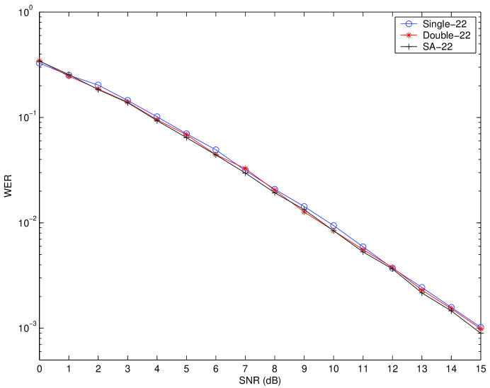
Figure 3: The maximum-likelihood word error rates (WERs) of the half-rate computer-searched code by simulated annealing in [18] (SA-22), the rule-based half-rate code with double code trees (Double-22), and the rule-based half-rate code with single code tree (Single-22). The codeword length is $N=22$.

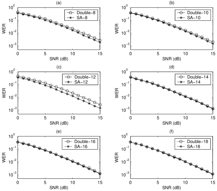
Figure 4: The maximum-likelihood word error rates (WERs) of the computer-searched half-rate code by simulated annealing (SA-$N$) and the rule-based half-rate code with double code trees (Double-$N$).

There are three codes simulated in Fig. 3: the computer-searched half-rate code obtained in [18] (SA-22), the rule-based double-tree code in which half of the codewords satisfying $\mathbb{B}^{T}\mathbb{B}=\mathbb{G}_{1}$ and the remaining half satisfying $\mathbb{B}^{T}\mathbb{B}=\mathbb{G}_{2}$ (Double-22), and the rule-based single-tree code whose codewords are all selected from the candidate sequences satisfying $\mathbb{B}^{T}\mathbb{B}=\mathbb{G}_{1}$ (Single-22). We observe from Fig. 3 that the Double-22 code performs almost the same as the SA-22 code obtained in [18] at $N=22$. Actually, extensive simulations in Fig. 4 show that the performance of the rule-based double-tree half-rate codes is as good as the computer-searched half-rate codes for all $N>12$. However, when $N\leq 12$, the approximation in (12) can no longer be well maintained due to the restriction that $|{\mathcal{A}}(\boldsymbol{b}_{(\ell)}|\mathbb{G})|$ must be an integer, and an apparent performance deviation between the rule-based double-tree half-rate codes and the computer-searched half-rate codes can therefore be sensed for $N$ below 12.

In addition to the Double-22 code, the performance of the Single-22 code is also simulated in Fig. 3. Since the pairwise codeword distance in the sense of (11) for the Single-22 code is in general smaller than that of the Double-22 code, its performance has $0.2$ dB degradation to that of the Double-22 code. However, we will see in later simulation that the Single-22 code has the smallest decoding complexity among the three codes in Fig. 3. This suggests that to select codewords uniformly from a single code tree should not be ruled out as a candidate design, especially when the decoding complexity becomes the main system concern.

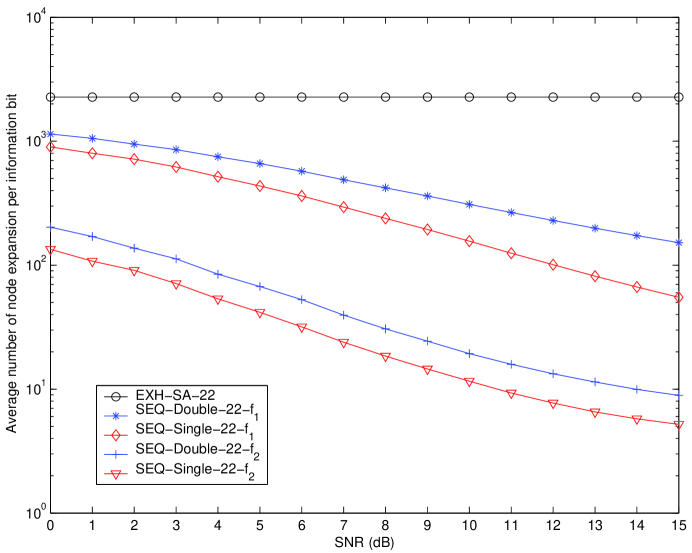
Figure 5: The average numbers of node expansions per information bit for the computer-searched code in [18] by exhaustive decoding (EXH-SA-22), and the rule-based single-tree (SEQ-Single-$22$) and double-tree (SEQ-Double-$22$) codes using the priority-first search decoding guided by either evaluation function $f_{1}$ or evaluation function $f_{2}$.

In Fig. 5, the average numbers of node expansions per information bit are illustrated for the codes examined in Fig. 3. Since the number of nodes expanded is exactly the number of tree branch metrics (i.e., one recursion of $f$-function values) computed, the equivalent complexity of exhaustive decoder is correspondingly plotted. It can then be observed that in comparison with the exhaustive decoder, a significant reduction in computational burdens can be obtained at moderate-to-high SNRs by adopting the Double-22 code and the priority-first search decoder with on-the-fly evaluation function $f_{1}$, namely, $g$ (cf. Eq. (17)). Further reduction can be approached if the Double-22 code is replaced with the Single-22 code. The is because performing the sequential search over multiple code trees introduce extra node expansions for those code trees that the transmitted codeword does not belong to. An additional order-of-magnitude reduction in node expansions can be achieved when the evaluation function $f_{2}=g+h_{2}$ is used instead.

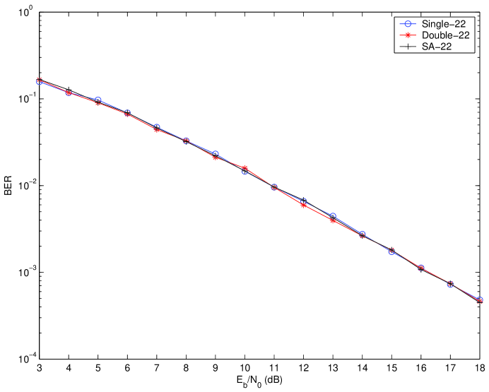
Figure 6: Bit error rates (BERs) for the codes simulated in Fig. 3.

The authors in [3] and [18] only focused on the word-error-rates (WERs). No bit error rate (BER) performances that involve the mapping design between the information bit patterns and the codewords were presented. Yet, in certain applications, such as voice transmission and digital radio broadcasting, the BER is generally considered a more critical performance index. In addition, the adoption of the BER performance index, as well as the signal-to-noise ratio per information bit, facilitates the comparison among codes of differen code rates.

Figure 6 depicts the BER performances of the codes simulated in Fig. 3. The corresponding $E_{b}/N_{0}$ is computed according to:

$$E_{b}/N_{0}=\frac{1}{R}\cdot\mbox{SNR},$$

where $R=K/N$ is the code rate. The mapping between the bit patterns and the codewords of the given computer-searched code is obtained through simulated annealing by minimizing the upper bound of:

$$\mbox{BER}\leq\frac{1}{2^{K}}\sum_{i=1}^{2^{K}}\sum_{j=1,j\neq i}^{2^{K}}\frac{D(\boldsymbol{m}(i),\boldsymbol{m}(j))}{K}\Pr\left(\left.\hat{\boldsymbol{b}}=\boldsymbol{b}(j)\right|\boldsymbol{b}(i)\mbox{ transmitted}\right),$$

where, other than the notations defined in (3), $\boldsymbol{m}(i)$ is the information sequence corresponding to $i$-th codeword, and $D(\cdot,\cdot)$ is the Hamming distance. For the rule-based constructed codes in Section III-C, the binary representation of the index of the requested codeword in Step 1 is directly taken as the information bit pattern corresponding to the requested codeword. The result in Fig. 6 then indicates that the BER performances of the three curves are almost the same, which directs the conclusion that taking the binary representation of the requested codeword index as the information bit pattern for the rule-based constructed code not only makes easy its implementation but also has similar BER performance to the computer-optimized codes.

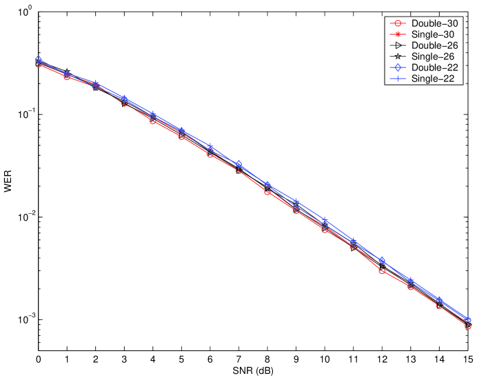
Figure 7: Word error rates (WERs) for the codes of Single-$22$, Double-$22$, Single-$26$, Double-$26$, Single-$30$ and Double-$30$.

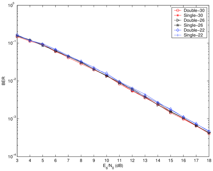
Figure 8: Bit error rates (BERs) for the codes of Single-$22$, Double-$22$, Single-$26$, Double-$26$, Single-$30$ and Double-$30$.

In the end, we demonstrate the WER and BER performances of Single-$26$, Double-$26$, Single-$30$, Double-$30$ codes, together with those of Single-$22$ and Double-$22$ codes, over the quasi-static fading channels respectively in Figs. 7 and 8. Both figures show that the Double-$30$ code has the best maximum-likelihood performance not only in WER but also in BER. This result echoes the usual anticipation that the performance favors a longer code as long as the channel coefficients remain unchanged in a coding block. Their decoding complexities are listed in Tab. I, from which we observe that the saving of decoding complexity of metric $f_{2}$ with respect to metric $f_{1}$ increases as the codeword length further grows.

TABLE I: Average numbers of node expansions per information bit for the priority-first search decoding of the constructed half-rate codes of length $22$, $26$ and $30$.

$SNR$	5dB	6dB	7dB	8dB	9dB	10dB	11dB	12dB	13dB	14dB	15dB
Double-22-$f_{1}$	671	590	506	436	375	320	274	236	204	178	156
Double-22-$f_{2}$	68	55	42	32	26	20	17	14	12	10	9
ratio of $\left.f_{1}\right/f_{2}$	9.8	10.7	12.0	13.6	14.4	16.0	16.1	16.8	17.0	17.8	17.3
Double-$26$-$f_{1}$	$2361$	$2006$	$1695$	$1416$	$1189$	$981$	$813$	$677$	523	499	392
Double-$26$-$f_{2}$	$175$	$130$	$94$	$69$	$53$	$39$	$29$	$23$	18	15	13
ratio of $\left.f_{1}\right/f_{2}$	$13.5$	$15.4$	$18.0$	$20.5$	$22.4$	$25.2$	$28.0$	$29.4$	29.1	33.3	30.2
Double-$30$-$f_{1}$	$8455$	$7073$	$5760$	$5133$	$3759$	$3430$	$2644$	$1996$	$1765$	$1368$	$1081$
Double-$30$-$f_{2}$	$459$	$332$	$232$	$166$	$119$	$86$	$60$	$44$	$33$	$25$	$20$
ratio of $\left.f_{1}\right/f_{2}$	$18.4$	$21.3$	$24.8$	$30.9$	$31.6$	$39.9$	$44.1$	$45.4$	$53.4$	$54.7$	$54.1$
Single-$22$-$f_{1}$	460	371	308	250	200	163	130	105	85	69	57
Single-$22$-$f_{2}$	45	33	26	20	15	12	10	8	7	6	5
ratio of$\left.f_{1}\right/f_{2}$	10.2	11.2	11.8	12.5	13.3	13.5	13.0	13.1	12.1	11.5	11.4
Single-$26$-$f_{1}$	$1635$	$1328$	$1061$	$839$	$666$	$522$	$403$	$312$	$244$	$191$	$152$
Single-$26$-$f_{2}$	$112$	$79$	$57$	$42$	$31$	$23$	$17$	$13$	$11$	$9$	$7$
ratio of $\left.f_{1}\right/f_{2}$	$14.6$	$16.8$	$18.6$	$20.0$	$21.5$	$22.7$	$23.7$	$23.9$	$22.2$	$21.2$	$21.7$
Single-$30$-$f_{1}$	$5871$	$4695$	$3857$	$2924$	$2335$	$1813$	$1328$	$884$	$805$	$572$	$416$
Single-$30$-$f_{2}$	$284$	$199$	$144$	$101$	$72$	$51$	$35$	$26$	18	14	11
ratio of $\left.f_{1}\right/f_{2}$	$20.6$	$23.6$	$26.8$	$29.0$	$32.4$	$35.5$	$38.0$	$34.0$	$44.7$	$40.9$	$37.8$

VI Codes for channels with fast fading

In previous sections, also in [2], [6] and [18], it is assumed that the channel coefficients $\boldsymbol{h}$ are invariant in each coding block of length $L=N+P-1$. In this section, we will show that the approaches employed in previous sections can also be applicable to the situation that $\boldsymbol{h}$ may change in every $Q$ symbol, where $Q<L$.

For $1\leq k\leq M=\lceil L/Q\rceil$, let $\boldsymbol{h}_{k}\triangleq[h_{1,k}\ \ h_{2,k}\ \cdots\ h_{P,k}]^{T}$ be the constant channel coefficients at the $k$th sub-block. Denote by $\boldsymbol{b}_{k}=[b_{(k-1)Q-P+2}\ \cdots\ b_{(k-1)Q+1}\ \cdots\ b_{kQ}]^{T}$ the portion of $\boldsymbol{b}$, which will affect the output portion $\boldsymbol{y}_{k}=[y_{(k-1)Q+1}\ \ y_{(k-1)Q+2}\ \cdots\ y_{kQ}]$, where we assume $b_{j}=0$ for $j\leq 0$ and $j>N$ for notational convenience. Then, for a channel whose coefficients change in every $Q$ symbol, the system model defined in (1) remains as $\boldsymbol{y}=\mathbb{B}\boldsymbol{h}+\boldsymbol{n}$ except that both $\boldsymbol{y}$ and $\boldsymbol{n}$ extend as $MQ\times 1$ vectors with $y_{j}=n_{j}=0$ for $j>L$, and $\mathbb{B}$ and $\boldsymbol{h}$ have to be re-defined as

$$\mathbb{B}\triangleq\mathbb{B}_{1}\oplus\mathbb{B}_{2}\oplus\cdots\oplus\mathbb{B}_{M}\quad{\rm and}\quad\boldsymbol{h}\triangleq\begin{bmatrix}\boldsymbol{h}_{1}^{H}&\boldsymbol{h}_{2}^{H}&\cdots&\boldsymbol{h}_{M}^{H}\end{bmatrix}^{H},$$

where $\mathbb{B}_{k}=[\boldsymbol{0}_{Q\times(P-1)}\ \ \mathbb{I}_{Q}][\boldsymbol{b}_{k}\ \ \tilde{\mathbb{E}}\boldsymbol{b}_{k}\ \cdots\ \tilde{\mathbb{E}}^{P-1}\boldsymbol{b}_{k}]$ is a $Q\times P$ matrix,

$$\tilde{\mathbb{E}}\triangleq\begin{bmatrix}0&0\cdots&0&0\\ 1&0\ddots&0&0\\ 0&1\ddots&0&0\\ 0&0\cdots&1&0\end{bmatrix}_{(Q+P-1)\times(Q+P-1)}$$

and “$\oplus$” is the direct sum operator of two matrices.

Based on the new system model, we have $\mathbb{P}_{B}=\mathbb{P}_{B_{1}}\oplus\mathbb{P}_{B_{2}}\oplus\cdots\oplus\mathbb{P}_{B_{M}}$, where $\mathbb{P}_{B_{k}}=\mathbb{B}_{k}(\mathbb{B}_{k}^{T}\mathbb{B}_{k})^{-1}\mathbb{B}_{k}^{T}$, and Eq. (9) becomes:

$$\hat{\boldsymbol{b}}=\arg\max_{\boldsymbol{b}\in\mathcal{C}}\sum_{k=1}^{M}\left\|\mathrm{vec}(\boldsymbol{y}_{k}\boldsymbol{y}_{k}^{H})-\mathrm{vec}(\mathbb{P}_{B_{k}})\right\|^{2}$$ (22)

Again, codeword $\boldsymbol{b}$ and transformed codeword $\mathbb{P}_{B}$ is not one-to-one corresponding unless the first element of $\boldsymbol{b}$, namely $b_{1}$, is fixed.

Since $\mathbb{B}^{T}\mathbb{B}=(\mathbb{B}_{1}^{T}\mathbb{B}_{1})\oplus(\mathbb{B}_{2}^{T}\mathbb{B}_{2})\oplus\cdots\oplus(\mathbb{B}_{M}^{T}\mathbb{B}_{M})$, the maximization of system SNR can be achieved simply by assigning

$$\mathbb{B}_{1}^{T}\mathbb{B}_{1}=\mathbb{B}_{2}^{T}\mathbb{B}_{2}=\cdots=\mathbb{B}_{M}^{T}\mathbb{B}_{M}=Q\cdot\mathbb{I}_{Q}$$ (23)

if such assignment is possible. Due to the same reason mentioned in Section III-A, approximation to (23) will have to be taken in the true code design.

It remains to determine the number of all possible $\pm 1$-sequences of length $N$, whose first $\ell$ bits equal $b_{1}$, $b_{2}$, $\ldots$, $b_{\ell}$ subject to $\mathbb{B}_{k}^{T}\mathbb{B}_{k}=\mathbb{G}_{k}$ for $1\leq k\leq M$.

Lemma 3

Fix $P=2$ and $Q\geq P$, and put

$$\mathbb{B}_{1}^{T}\mathbb{B}_{1}=\begin{bmatrix}Q&c_{1}\\ c_{1}&Q-1\end{bmatrix},\quad\mathbb{B}_{k}^{T}\mathbb{B}_{k}=\begin{bmatrix}Q&c_{k}\\ c_{k}&Q\end{bmatrix}\mbox{ for }2\leq k\leq M-1,\quad$$

$$\mbox{and }\mathbb{B}_{M}^{T}\mathbb{B}_{M}=\begin{bmatrix}N-(M-1)Q&c_{M}\\ c_{M}&N-(M-1)Q+1\end{bmatrix},$$ (24)

where in our code selection process, $[c_{1},c_{2},\cdots,c_{M}]\in\{0,\pm 1\}^{M}$ will be chosen such that $Q-1+c_{1}$, $Q+c_{k}$ for $2\leq k\leq M-1$, and $N-(M-1)Q+c_{M}$ are all even. Then, the number of all possible $\pm 1$-sequences of length $N$, whose first $\ell$ bits equal $b_{1}$, $b_{2}$, $\ldots$, $b_{\ell}$ subject to (24) is given by:

$$\left\{\begin{array}[]{r}\displaystyle\binom{Q-(\ell\bmod Q)}{\frac{Q-(\ell\bmod Q)+c_{\tau}-m_{\ell}}{2}}\left[\displaystyle\prod_{k=\tau+1}^{M-1}\binom{Q}{\frac{Q+c_{k+1}}{2}}\right]\displaystyle\binom{N-(M-1)Q}{\frac{N-(M-1)Q+c_{M}}{2}}{\bf 1}\left\{|c_{\tau}-m_{\ell}|\leq Q-(\ell\bmod Q)\right\},\\ \mbox{ for }1\leq\tau<M;\\ \displaystyle\binom{N-(M-1)Q}{\frac{N-(M-1)Q+c_{M}-m_{\ell}}{2}}{\bf 1}\left\{|c_{M}-m_{\ell}|\leq N-(M-1)Q\right\},\hskip 128.0374pt\mbox{ for }\tau=M\\ \end{array}\right.$$

where $\tau=\lfloor\ell/Q\rfloor+1$, and

$$m_{\ell}=\left\{\begin{array}[]{ll}0,&\ell=1\mbox{ or }(\ell=(\tau-1)Q\mbox{ and }2\leq\tau\leq M);\\ b_{1}b_{2}+\cdots+b_{\ell-1}b_{\ell},&1<\ell<Q;\\ b_{(\tau-1)Q}b_{(\tau-1)Q+1}+\cdots+b_{\ell-1}b_{\ell},&(\tau-1)Q<\ell<\tau Q\mbox{ and }2\leq\tau\leq M.\end{array}\right.$$

Proof:

It requires

$$\left\{\begin{array}[]{lcl}c_{1}&=&b_{1}b_{2}+\cdots+b_{Q-1}b_{Q}\\ &\vdots&\\ c_{\tau}&=&b_{(\tau-1)Q}b_{(\tau-1)Q+1}+\cdots+b_{\ell}b_{\ell+1}+\cdots+b_{\tau Q-1}b_{\tau Q}\\ &=&m_{\ell}+b_{\ell}b_{\ell+1}+\cdots+b_{\tau Q-1}b_{\tau Q}\\ &\vdots&\\ c_{M}&=&b_{(M-1)Q}b_{(M-1)Q+1}+\cdots+b_{N-1}b_{N}\end{array}\right.$$

Following the same argument as in Lemma 2, we obtain that the number of all possible $\pm 1$-sequences of length $N$, whose first $\ell$ bits equal $b_{1}$, $b_{2}$, $\ldots$, $b_{\ell}$ subject to (24) is given by:

$$\binom{kQ-\ell}{(kQ-\ell+c_{k}-m_{\ell})/2}{\bf 1}\left\{|c_{k}-m_{\ell}|\leq kQ-\ell\right\}$$

$$\times\binom{Q}{(Q+c_{k+1})/2}{\bf 1}\left\{|c_{k+1}|\leq Q\right\}\times\cdots\times\binom{Q}{(Q+c_{M-1})/2}{\bf 1}\left\{|c_{M-1}|\leq Q\right\}$$

$$\times\binom{N-(M-1)Q}{(N-(M-1)Q+c_{M})/2}{\bf 1}\left\{|c_{M}|\leq N-(M-1)Q\right\}.$$

The proof is completed by noting that $\ell=(\tau-1)Q+(\ell\bmod Q)$, $|c_{k}|\leq Q$ and $|c_{M}|\leq N-(M-1)Q$ are always valid. ∎

With the availability of the above lemma, the code construction algorithm in Section III-C can be performed. Next, we re-derive the maximum-likelihood decoding metric for use of priority-first search decoding algorithm. Continuing the derivation from (22) based on $\mathbb{B}_{k}^{T}\mathbb{B}_{k}=\mathbb{G}_{\theta,k}$ for $1\leq k\leq M$ and $1\leq\theta\leq\Theta$, we can establish in terms of similar procedure as in Section IV-A that:

$$\hat{\boldsymbol{b}} = \arg\min_{\boldsymbol{b}\in\mathcal{C}}\frac{1}{2}\sum_{k=1}^{M}\sum_{m=1}^{Q+P-1}\sum_{n=1}^{Q+P-1}\left[-w_{m,n,k}^{(\theta)}b_{(k-1)Q-P+m+1}b_{(k-1)Q-P+n+1}\right]{\bf 1}\{\boldsymbol{b}\in{\mathcal{C}}_{\theta}\}$$

where for $1\leq m,n\leq Q+P-1$,

$$w_{m,n,k}^{(\theta)}=\sum_{i=0}^{P-1}\sum_{j=0}^{P-1}\delta_{i,j,k}^{(\theta)}\mathrm{Re}\{\tilde{y}_{m+i,k}\tilde{y}_{n+j,k}^{\ast}\},$$

$\delta_{i,j,k}^{(\theta)}$ is the $(i,j)$th entry of $\mathbb{D}_{\theta,k}=\mathbb{G}_{\theta,k}^{-1}$, and $\tilde{\boldsymbol{y}}_{k}=[\boldsymbol{0}_{1\times(P-1)}\ \ \boldsymbol{y}_{k}^{H}\ \ \boldsymbol{0}_{1\times(P-1)}]^{H}=[\tilde{y}_{1,k}\ \cdots\ \tilde{y}_{Q+2P-2,k}]^{T}$. As it turns out, the recursive on-the-fly metric for the priority-first search decoding algorithm is:

$$g(\boldsymbol{b}_{(\ell)})-g(\boldsymbol{b}_{(\ell-1)})=\left\{\begin{array}[]{r}\displaystyle\max_{1\leq\eta\leq\Theta}\alpha_{s,k}^{(\eta)}-b_{\ell}\sum_{i=0}^{P-1}\sum_{j=0}^{P-1}\delta_{i,j,k}^{(\theta)}\mathrm{Re}\{\tilde{y}_{s+i,k}\cdot u_{j,k}(\boldsymbol{b}_{(\ell)})\},\mbox{ for }P\leq s\leq Q\\ \displaystyle\max_{1\leq\eta\leq\Theta}\alpha_{r,k}^{(\eta)}+\max_{1\leq\eta\leq\Theta}\alpha_{s,k+1}^{(\eta)}-b_{\ell}\sum_{i=0}^{P-1}\sum_{j=0}^{P-1}\bigg{(}\delta_{i,j,k}^{(\theta)}\mathrm{Re}\{\tilde{y}_{r+i,k}\cdot u_{j,k}(\boldsymbol{b}_{(\ell)})\}\\ ~{}+\delta_{i,j,k+1}^{(\theta)}\mathrm{Re}\{\tilde{y}_{s+i,k+1}\cdot u_{j,k+1}(\boldsymbol{b}_{(\ell)})\}\bigg{)},\mbox{ otherwise.}\end{array}\right.$$

where $-P+2\leq\ell\leq N$, $s=[(\ell+P-2)\bmod Q]+1$, $r=s+Q$, $k=\max\{\lceil\ell/Q\rceil,1\}$,

$$\alpha_{s,k}^{(\eta)}\triangleq\sum_{n=1}^{s-1}\left|w_{s,n,k}^{(\eta)}\right|+\frac{1}{2}\left|w_{s,s,k}^{(\eta)}\right|$$

and

$$u_{j,k}(\boldsymbol{b}_{(\ell+1)})\triangleq u_{j,k}(\boldsymbol{b}_{(\ell)})+\frac{1}{2}\left(b_{\ell}\tilde{y}_{s+j,k}^{\ast}+b_{\ell+1}\tilde{y}_{s+j+1,k}^{\ast}\right)$$

with initial values $g(\boldsymbol{b}_{(-P+1)})=0$ and $u_{j,k}(\boldsymbol{b}_{((k-1)Q-P+2)})=0$ for $0\leq j\leq P-1$ and $1\leq k\leq M$. In addition, the low-complexity heuristic function is given by:

$$h_{2}(\boldsymbol{b}_{(\ell)})\triangleq\left\{\begin{array}[]{ll}\displaystyle\sum_{m=s+1}^{Q+P-1}\max_{1\leq\eta\leq\Theta}\alpha_{m,k}^{(\eta)}-\sum_{m=s+1}^{Q+P-1}\left|v_{m,k}^{(\theta)}(\boldsymbol{b}_{(\ell)})\right|-\beta_{s,k}^{(\theta)}&\\ \hskip 28.45274pt+\displaystyle\sum_{\kappa=k+1}^{M}\left(\sum_{m=1}^{Q+P-1}\max_{1\leq\eta\leq\theta}\alpha_{m,\kappa}^{(\eta)}-\beta_{0,\kappa}^{(\theta)}\right),&\mbox{for }P\leq s\leq Q;\\ \displaystyle\sum_{m=s+1}^{Q+P-1}\max_{1\leq\eta\leq\Theta}\alpha_{m,k+1}^{(\eta)}-\sum_{m=s+1}^{Q+P-1}\left|v_{m,k+1}^{(\theta)}(\boldsymbol{b}_{(\ell)})\right|-\beta_{s,k+1}^{(\theta)}&\\ \hskip 28.45274pt+\displaystyle\sum_{m=r+1}^{Q+P-1}\max_{1\leq\eta\leq\Theta}\alpha_{m,k}^{(\eta)}-\sum_{m=r+1}^{Q+P-1}\left|v_{m,k}^{(\theta)}(\boldsymbol{b}_{(\ell)})\right|-\beta_{r,k}^{(\theta)}&\\ \hskip 28.45274pt+\displaystyle\sum_{\kappa=k+2}^{M}\left(\sum_{m=1}^{Q+P-1}\max_{1\leq\eta\leq\theta}\alpha_{m,\kappa}^{(\eta)}-\beta_{0,\kappa}^{(\theta)}\right),&\mbox{otherwise},\end{array}\right.$$

where $s$, $r$ and $k$ are defined the same as for $g(\cdot)$,

$$v_{m,k}^{(\theta)}(\boldsymbol{b}_{(\ell)})\triangleq\sum_{n=1}^{s}w_{m,n,k}^{(\theta)}b_{(k-1)Q+P+n-1}=v_{m,k}^{(\theta)}(\boldsymbol{b}_{(\ell-1)})+w_{s,m,k}^{(\theta)}b_{\ell},$$

and

$$\beta_{s,k}^{(\theta)}\triangleq\sum_{m=s+1}^{Q+P-1}\left(\sum_{n=s+1}^{m-1}\left|w_{m,n,k}^{(\theta)}\right|+\frac{1}{2}\left|w_{m,m,k}^{(\theta)}\right|\right)=\beta_{s-1,k}^{(\theta)}-\sum_{n=s+1}^{Q+P-1}\left|w_{s,n,k}^{(\theta)}\right|-\frac{1}{2}\left|w_{s,s,k}^{(\theta)}\right|$$

with initial values $v_{m,k}^{(\theta)}(\boldsymbol{b}_{(k-1)Q-P+2})=0$ and $\beta_{0,k}^{(\theta)}=\sum_{m=1}^{Q+P-1}\alpha_{m,k}^{(\theta)}$.

It is worth mentioning that if the single-tree code is adopted, $h_{2}(\cdot)$ can be further reduced to:

$$h_{2}(\boldsymbol{b}_{(\ell)}) \triangleq \left\{\begin{array}[]{ll}\displaystyle\sum_{m=s+1}^{Q+P-1}\alpha_{m,k}^{(1)}-\sum_{m=s+1}^{Q+P-1}\left|v_{m,k}^{(1)}(\boldsymbol{b}_{(\ell)})\right|-\beta_{s,k}^{(1)}&\mbox{for }P\leq s\leq Q;\\ \displaystyle\sum_{m=s+1}^{Q+P-1}\alpha_{m,k+1}^{(1)}-\sum_{m=s+1}^{Q+P-1}\left|v_{m,k+1}^{(1)}(\boldsymbol{b}_{(\ell)})\right|-\beta_{s,k+1}^{(1)}&\\ \hskip 28.45274pt+\displaystyle\sum_{m=r+1}^{Q+P-1}\alpha_{m,k}^{(1)}-\sum_{m=r+1}^{Q+P-1}\left|v_{m,k}^{(1)}(\boldsymbol{b}_{(\ell)})\right|-\beta_{r,k}^{(1)}&\mbox{otherwise},\end{array}\right.$$

since $\sum_{m=1}^{Q+P-1}\max_{1\leq\eta\leq\theta}\alpha_{m,\kappa}^{(\eta)}-\beta_{0,\kappa}^{(\theta)}=\sum_{m=1}^{Q+P-1}\alpha_{m,\kappa}^{(1)}-\beta_{0,\kappa}^{(1)}=0;$ hence, a sub-blockwise low-complexity on-the-fly decoding can indeed be conducted under the single code tree condition.

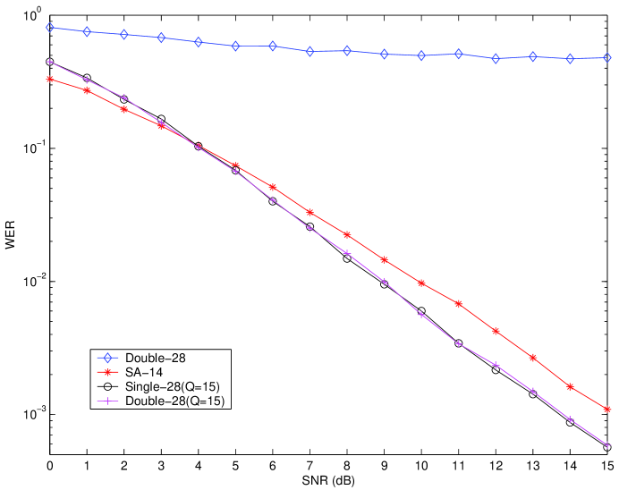
Figure 9: Word error rates (BERs) for the codes of Double-$28$, SA-$14$, Single-$28$($Q$=15) and Double-$28$($Q$=15) over the quasi-static channel with $Q_{\rm chan}=15$.

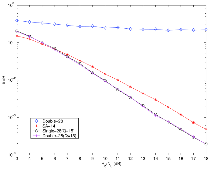
Figure 10: Bit error rates (BERs) for the codes of Double-$28$, SA-$14$, Single-$28$($Q$=15) and Double-$28$($Q$=15) over the quasi-static channel with $Q_{\rm chan}=15$.

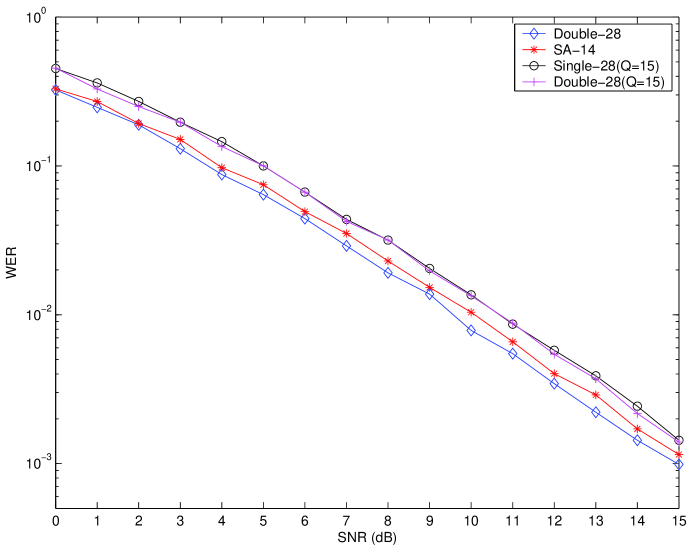
Figure 11: Word error rates (BERs) for the codes of Double-$28$, SA-$14$, Single-$28$($Q$=15) and Double-$28$($Q$=15) over the quasi-static channel with $Q_{\rm chan}\geq 29$.

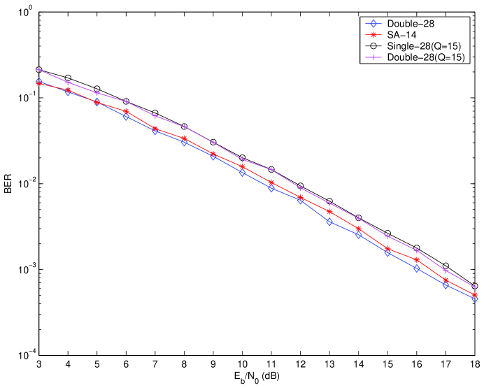
Figure 12: Bit error rates (BERs) for the codes of Double-$28$, SA-$14$, Single-$28$($Q$=15) and Double-$28$($Q$=15) over the quasi-static channel with $Q_{\rm chan}\geq 29$.

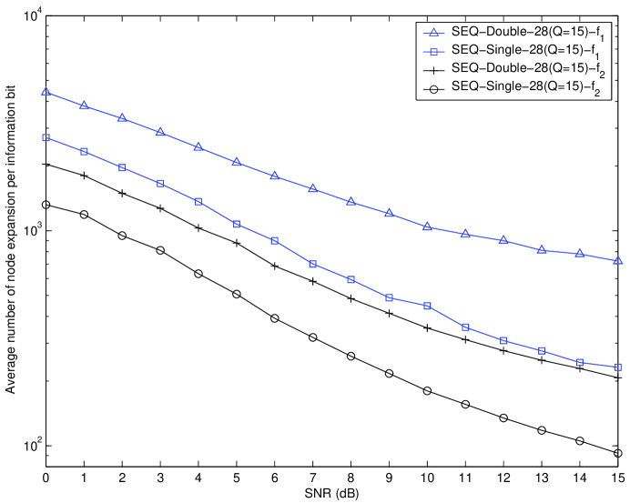
Figure 13: Average numbers of node expansions per information bit for the codes of Single-28($Q$=15) and Double-28($Q$=15) using the priority-first search decoding guided by either evaluation function $f_{1}$ or evaluation function $f_{2}$ over the quasi-static channel with $Q_{\rm chan}=15$.

Figures 9 and 10 compare four codes over fading channels whose channel coefficients vary in every $15$-symbol period. Notably, we will use $Q_{\rm chan}$ to denote the varying period of the channel coefficients $\boldsymbol{h}$, and retain $Q$ as the design parameter for the nonlinear codes. In notations, “Double-$28$” and “SA-$14$” denote the codes defined in the previous sections, and “Single-$28$($Q$=15)” and “Double-$28$($Q$=15)” are the codes constructed based on the rule introduced in this section under the design parameter $Q=15$. Again, the mapping between the bit patterns and codewords for the SA-$14$ code is defined by simulated annealing.

Both Figs. 9 and 10 show that the Double-$28$ code seriously degrades when the channel coefficients unexpectedly vary in an intra-codeword fashion. This hints that the assumption that the channel coefficients remain constant in a coding block is critical in the code design in Section III. Figures 11 and 12 then indicate that the codes taking into considerations the varying nature of the channel coefficients within a codeword is robust in its performance when being applied to channels with constant coefficients. Thus, we may conclude that for a channel whose coefficients vary more often than a coding block, it is advantageous to use the code design for a fast-fading environment considered in the section.

A more striking result from Fig. 9 is that even if the codeword length of the Single-28($Q$=15) and the Double-28($Q$=15) codes is twice of the SA-14 code, their word error rates are still markedly superior at medium-to-high SNRs. Note that the SA-14 code is the computer-optimized code specifically for $Q_{\rm chan}=15$ channel. This hints that when the channel memory order is known, performance gain can be obtained by considering the inter-subblock correlation, and favors a longer code design.

The decoding complexity, measured in terms of average number of node expansions per information bit, for codes of Single-28($Q$=15) and Double-28($Q$=15) are illustrated in Fig. 13. Similar observation is attained that the decoding metric $f_{2}$ yields less decoding complexity than the on-the-fly decoding one $f_{1}$.

VII Conclusions

In this paper, we established the systematic rule to construct codes based on the optimal signal-to-noise ratio framework that requires every codeword to satisfy a “self-orthogonal” property to combat the multipath channel effect. Enforced by this structure, we can then derive a recursive maximum-likelihood metric for the tree-based priority-first search decoding algorithm, and hence, avoid the use of the time-consuming exhaustive decoder that was previously used in [3, 6, 18] to decode the structureless computer-optimized codes. Simulations demonstrate that the ruled-based codes we constructed has almost identical performance to the computer-optimized codes, but its decoding complexity, as anticipated, is much lower than the exhaustive decoder.

Moreover, two maximum-likelihood decoding metrics were actually proposed. The first one can be used in an on-the-fly fashion, while the second one as having a much less decoding complexity requires the knowledge of all channel outputs. The trade-off between them is thus evident from our simulations.

Extensions of the code design to a fast-varying quasi-static environment is added in Section VI. Although we only derive the coding rule and its decoding metric for a fixed $Q$, further extension to the situation that the channel coefficients $\boldsymbol{h}$ vary non-stationarily as the periods $Q_{1}$, $Q_{2}$, $\ldots$, $Q_{M}$ are not equal is straightforward. Such design may be suitable for, e.g., the frequency-hopping scheme of Global System for Mobile communications (GSM) and Universal Mobile Telecommunications System (UMTS), and the time-hopping scheme in IS-$54$, in which cases the channel coefficients change (or hop) at protocol-aware scheduled time instants as similarly mentioned in [12].

A limitation on the code design we proposed is that the decoding complexity grows exponentially with the codeword length. This constraint is owning to the tree structure of our constructed codes. It will be an interesting and useful future work to re-design the self-orthogonal codes that can be fit into a trellis structure, and make them maximum-likelihood decodable by either the priority-first search algorithm or the Viterbi-based algorithm.

Appendix

Lemma 4

Fix $P>1$ and $k\geq 1$. For given integers $\boldsymbol{q}=(q_{1}$, $q_{2}$, $\cdots$, $q_{P-1})\in[-k,k]^{P-1}$ and $d_{2-P}$, $d_{3-P}$, $\cdots$, $d_{0}\in\{\pm 1\}$, let the number of $d_{1},d_{2},\cdots,d_{k}$ that simultaneously satisfy

$$q_{j} = \sum_{i=1}^{k}d_{i-j}d_{i}\mbox{ for }1\leq j\leq P-1$$

be denoted by $A_{k}(\boldsymbol{q}|d_{2-P},\cdots,d_{0})$. Also, let $\mathbb{G}(\boldsymbol{c})$ be the $P\times P$ matrix of the Toeplitz form:

$$\mathbb{G}(\boldsymbol{c})=\begin{bmatrix}N&c_{1}&c_{2}&\cdots&c_{P-1}\\ c_{1}&N&c_{1}&\cdots&c_{P-2}\\ c_{2}&c_{1}&N&\cdots&c_{P-3}\\ \vdots&\vdots&\vdots&\ddots&\vdots\\ c_{P-1}&c_{P-2}&c_{P-3}&\cdots&N\end{bmatrix},$$

where $\boldsymbol{c}=(c_{1},c_{2},\cdots,c_{P-1})\in\{\pm 1\}^{P-1}$. Then, for $\ell=1,2,\cdots,N$,

$$|{\mathcal{A}}(\boldsymbol{b}_{(\ell)}|\mathbb{G}(\boldsymbol{c}))|=A_{N-\ell}\left(\boldsymbol{c}-\boldsymbol{m}_{\ell}\left|b_{\ell-P+2},\cdots,b_{\ell}\right.\right).$$

where $\boldsymbol{m}_{\ell}=(m_{\ell}^{(1)},\cdots,m_{\ell}^{(P-1)})$ and $m_{\ell}^{(k)}\triangleq(b_{1}b_{k+1}+\cdots+b_{\ell-k}b_{\ell})\cdot{\bf 1}\{\ell>k\}$.

Proof:

For $\mathbb{B}^{T}\mathbb{B}=\mathbb{G}(\boldsymbol{c})$, it requires

$$c_{1} = b_{1}b_{2}+b_{2}b_{3}+\cdots+b_{N-1}b_{N}=m_{\ell}^{(1)}+b_{\ell}b_{\ell+1}+\cdots+b_{N-1}b_{N}$$

$$c_{2} = b_{1}b_{3}+b_{2}b_{4}+\cdots+b_{N-2}b_{N}=m_{\ell}^{(2)}+b_{\ell-1}b_{\ell+1}+\cdots+b_{N-2}b_{N}$$

$$\vdots$$

$$c_{P-1} = b_{1}b_{P}+b_{2}b_{P+1}+\cdots+b_{N-P+1}b_{N}=m_{\ell}^{(P-1)}+b_{\ell-P+2}b_{\ell+1}+\cdots+b_{N-P+1}b_{N}.$$

Re-writing the above equations as:

$$c_{1}-m_{\ell}^{(1)} = b_{\ell}b_{\ell+1}+\cdots+b_{N-1}b_{N}$$

$$c_{2}-m_{\ell}^{(2)} = b_{\ell-1}b_{\ell+1}+\cdots+b_{N-2}b_{N}$$

$$\vdots$$

$$c_{P-1}-m_{\ell}^{(P-1)} = b_{\ell-P+2}b_{\ell+1}+\cdots+b_{N-P+1}b_{N},$$

we obtain:

$$|{\mathcal{A}}(\boldsymbol{b}_{(\ell)}|\mathbb{G}(\boldsymbol{c}))|=A_{N-\ell}\left(\boldsymbol{c}-\boldsymbol{m}_{\ell}\left|b_{\ell-P+2},\cdots,b_{\ell}\right.\right).$$

∎

It can be easily verified that $A_{k}(\boldsymbol{q}|-d_{2-P},\cdots,-d_{0})=A_{k}(\boldsymbol{q}|d_{2-P},\cdots,d_{0})$ since

$$q_{j}=\sum_{i=1}^{j}(-d_{i-j})d_{i}+\sum_{i=j+1}^{k}d_{i-j}d_{i}=\sum_{i=1}^{j}d_{i-j}(-d_{i})+\sum_{i=j+1}^{k}(-d_{i-j})(-d_{i}).$$

Therefore, only $2^{P-2}$ tables are required. The tables of $A_{k}(\boldsymbol{q}|d_{-P+2},\cdots,d_{0})$ for $P=3$ and $1\leq k\leq 5$ are illustrated in Table II as an example.

TABLE II: Tables of $A_{k}(\boldsymbol{q}|d_{-1},d_{0})$ for $P=3$.

		$q_{2}$
​​​​$A_{1}(\cdot|-1,-1)$​​​​		$-1$	$0$	$1$
	$-1$	1	0	0
$q_{1}$	$0$	0	0	0
	$1$	0	0	1

		$q_{2}$
​​​​$A_{1}(\cdot|-1,1)$​​​​		$-1$	$0$	$1$
	$-1$	0	0	1
$q_{1}$	$0$	0	0	0
	$1$	1	0	0

		$q_{2}$
​​​​$A_{2}(\cdot|-1,-1)$​​​​		$-2$	$-1$	$0$	$1$	$2$
	$-2$	0	0	1	0	0
	$-1$	0	0	0	0	0
$q_{1}$	$0$	1	0	1	0	0
	$1$	0	0	0	0	0
	$2$	0	0	0	0	1

		$q_{2}$
​​​​$A_{2}(\cdot|-1,1)$​​​​		$-2$	$-1$	$0$	$1$	$2$
	$-2$	0	0	0	0	1
	$-1$	0	0	0	0	0
$q_{1}$	$0$	1	0	1	0	0
	$1$	0	0	0	0	0
	$2$	0	0	1	0	0

$q_{2}$ ​​​​$A_{3}(\cdot|-1,-1)$​​​​ $-3$ $-2$ $-1$ $0$ $1$ $2$ $3$ $-3$ 0 0 0 0 1 0 0 $-2$ 0 0 0 0 0 0 0 $-1$ 1 0 1 0 1 0 0 $q_{1}$ $0$ 0 0 0 0 0 0 0 $1$ 0 0 2 0 1 0 0 $2$ 0 0 0 0 0 0 0 $3$ 0 0 0 0 0 0 1   $q_{2}$ ​​​​$A_{3}(\cdot|-1,1)$​​​​ $-3$ $-2$ $-1$ $0$ $1$ $2$ $3$ $-3$ 0 0 0 0 0 0 1 $-2$ 0 0 0 0 0 0 0 $-1$ 0 0 2 0 1 0 0 $q_{1}$ $0$ 0 0 0 0 0 0 0 $1$ 1 0 1 0 1 0 0 $2$ 0 0 0 0 0 0 0 $3$ 0 0 0 0 1 0 0 $\vdots$
$q_{2}$ ​​​​$A_{4}(\cdot|-1,-1)$​​​​ $-4$ $-3$ $-2$ $-1$ $0$ $1$ $2$ $3$ $4$ $-4$ 0 0 0 0 0 0 1 0 0 $-3$ 0 0 0 0 0 0 0 0 0 $-2$ 0 0 2 0 1 0 1 0 0 $-1$ 0 0 0 0 0 0 0 0 0 $q_{1}$ $0$ 1 0 2 0 2 0 1 0 0 $1$ 0 0 0 0 0 0 0 0 0 $2$ 0 0 0 0 3 0 1 0 0 $3$ 0 0 0 0 0 0 0 0 0 $4$ 0 0 0 0 0 0 0 0 1   $q_{2}$ ​​​​$A_{4}(\cdot|-1,1)$​​​​ $-4$ $-3$ $-2$ $-1$ $0$ $1$ $2$ $3$ $4$ $-4$ 0 0 0 0 0 0 0 0 1 $-3$ 0 0 0 0 0 0 0 0 0 $-2$ 0 0 0 0 3 0 1 0 0 $-1$ 0 0 0 0 0 0 0 0 0 $q_{1}$ $0$ 1 0 2 0 2 0 1 0 0 $1$ 0 0 0 0 0 0 0 0 0 $2$ 0 0 2 0 1 0 1 0 0 $3$ 0 0 0 0 0 0 0 0 0 $4$ 0 0 0 0 0 0 1 0 0 $\vdots$
$q_{2}$ ​​​​$A_{5}(\cdot|-1,-1)$​​​​ $-5$ $-4$ $-3$ $-2$ $-1$ $0$ $1$ $2$ $3$ $4$ $5$ $-5$ 0 0 0 0 0 0 0 0 1 0 0 $-4$ 0 0 0 0 0 0 0 0 0 0 0 $-3$ 0 0 0 0 3 0 1 0 1 0 0 $-2$ 0 0 0 0 0 0 0 0 0 0 0 $-1$ 1 0 2 0 4 0 2 0 1 0 0 $q_{1}$ $0$ 0 0 0 0 0 0 0 0 0 0 0 $1$ 0 0 3 0 3 0 3 0 1 0 0 $2$ 0 0 0 0 0 0 0 0 0 0 0 $3$ 0 0 0 0 0 0 4 0 1 0 0 $4$ 0 0 0 0 0 0 0 0 0 0 0 $5$ 0 0 0 0 0 0 0 0 0 0 1   $q_{2}$ ​​​​$A_{5}(\cdot|-1,1)$​​​​ $-5$ $-4$ $-3$ $-2$ $-1$ $0$ $1$ $2$ $3$ $4$ $5$ $-5$ 0 0 0 0 0 0 0 0 0 0 1 $-4$ 0 0 0 0 0 0 0 0 0 0 0 $-3$ 0 0 0 0 0 0 4 0 1 0 0 $-2$ 0 0 0 0 0 0 0 0 0 0 0 $-1$ 0 0 3 0 3 0 3 0 1 0 0 $q_{1}$ $0$ 0 0 0 0 0 0 0 0 0 0 0 $1$ 1 0 2 0 4 0 2 0 1 0 0 $2$ 0 0 0 0 0 0 0 0 0 0 0 $3$ 0 0 0 0 3 0 1 0 1 0 0 $4$ 0 0 0 0 0 0 0 0 0 0 0 $5$ 0 0 0 0 0 0 0 0 1 0 0

References

• [1] J. B. Anderson and S. Mohan, “Sequential coding algorithms: A survey and cost analysis,” IEEE Trans. Commun., vol. 32, no. 2, pp. 169-176, February 1984.
• [2] K. M. Chugg and A. Polydoros, “MLSE for an unknown channel-part I: Optimality considerations,” IEEE Trans. Commun., vol. 44, no. 7, pp. 836-846, July 1996.
• [3] O. Coskun and K. M. Chugg, “Combined coding and training for unknown ISI channels,” IEEE Trans. Commun., vol. 53, no. 8, pp. 1310-1322, Auguest 2005.
• [4] S. N. Crozier and D. D. Falconer and S. A. Mahmound, “Least sum of squared errors (LSSE) channel estimation,” Proc. Inst. Elect. Eng., vol. 138, pt. F, pp. 371-378, Auguest 1991.
• [5] G. Ganesan and P. Stoica, “Space-time block codes: A maximum SNR approach,” IEEE Trans. Inform. Theory, vol. 47, no. 4, pp. 1650-1659, May 2001.
• [6] J. Giese and M. Skoglund, “Single- and multiple-antenna constellations for communication over unknown frequency-selective fading channels,” IEEE Trans. Inform. Theory, vol. 53, no. 4, pp. 1584-1594, April 2007.
• [7] Y. S. Han and C. R. P. Hartmann and C.-C. Chen, “Efficient priority-first search maximum-likelihood soft-decision decoding of linear block codes,” IEEE Trans. Inform. theory, vol. 39, no. 5, pp. 1514–1523, September 1993.
• [8] Y. S. Han and P.-N. Chen, “Sequential decoding of convolutional codes,” The Wiley Encyclopedia of Telecommunications, edited J. Proakis, John Wiley and Sons, Inc., 2002.
• [9] Y. S. Han, P.-N. Chen and H. -B. Wu, “A maximum-likelihood soft-decision sequential decoding algorithm for binary convolutional codes,” IEEE Trans. Communications, vol. 50, no. 2, pp. 173-178, February 2002.
• [10] D. Harville, Matrix Algebra From a Statistician’s Perspective, 1st edition, Springer, 2000.
• [11] C. Heegard, S. Coffey, S. Gummadi and E. J. Rossin, M. B. Shoemake and M. Wilhoyte, “Combined equalization and decoding for IEEE 802.11b devices,” IEEE J. Select. Areas Commun., vol. 21, no. 2, pp. 125-138, February 2003.
• [12] R. Knopp and P. A. Humblet “On coding for block fading channels,” IEEE Trans. Inform. Theory , vol. 46, no. 1, pp. 189-205, January 2000.
• [13] J. C. L. Ng, K. B. Letaief and R. D. Murch, “Complex optimal sequences with constant magnitude for fast channel estimation initialization,” IEEE Trans. commun., vol. 46, no. 3, pp. 305-308, March 1998.
• [14] S. I. Park, S. R. Park, I. Song and N. Suehiro, “Multiple-access interference reduction for QS-CDMA systems with a novel class of polyphase sequence,” IEEE Trans. Inform. Theory, vol. 46, no. 4, pp. 1448-1458, July 2000.
• [15] R. Patel and M. Toda, “Trace inequalities involving Hermitian metrices,” Linear Alg. Its Applic., vol. 23, pp. 13-20, 1979.
• [16] J. Proakis, Digital Communications, McGraw-Hill, fourth edition, 2001.
• [17] N. Seshadri, “Joint data and channel estimation using blind trellis search techniques,” IEEE Trans. Commun. , vol. 42, no. 2/3/4, pp. 1000-1011, February/March/April 1994.
• [18] M. Skoglund, J. Giese and S. Parkvall, “Code design for combined channel estimation and error protection,” IEEE Trans. Inform. Theory, vol. 48, no. 5, pp. 1162-1171, May 2002.
• [19] C. Tellambura, Y. J. Guo, and S. K. Barton, “Channel estimation using aperiodic binary sequences,” IEEE Commun. Letters, vol. 2, no. 5, pp. 140-142, May 1998.
• [20] C. Tepedelenlio$\breve{\rm g}$lu, A. Abdi and G. B. Giannakis, “The Ricean $K$ factor: Estimation and performance analysis,” IEEE Trans. Wireless Commun., vol. 2, no. 4, pp. 799-810, July 2003.
• [21] S.-A. Yang and J. Wu, “Optimal binary training sequence design for multiple-Antenna systems over dispersive fading channels,” IEEE Trans. Vehicular Technology, vol. 51, no. 5, pp. 1271-1276, September 2002.