Broadband microwave burst produced by electron beams

Abstract

Theoretical and experimental study of fast electron beams attracts a lot of attention in the astrophysics and laboratory. In the case of solar flares the problem of reliable beam detection and diagnostics is of exceptional importance. This paper explores the fact that the electron beams moving oblique to the magnetic field or along the field with some angular scatter around the beam propagation direction can generate microwave continuum bursts via gyrosynchrotron mechanism. The characteristics of the microwave bursts produced by beams differ from those in case of isotropic or loss-cone distributions, which suggests a new tool for quantitative diagnostics of the beams in the solar corona. To demonstrate the potentiality of this tool, we analyze here a radio burst occurred during an impulsive flare 1B/M6.7 on 10 March 2001 (AR 9368, N27W42). The burst is remarkably suitable for this goal because of its very short duration, wide frequency band and unusual polarization being in the ordinary wave mode in the optically thin range of the spectrum. Based on detailed analysis of the spectral, temporal, and spatial relationships, we obtained firm evidence that the microwave continuum burst is produced by electron beams. For the first time we developed and applied a new forward fitting algorithm based on exact gyrosynchrotron formulae and employing both the total power and polarization measurements to solve the inverse problem of the beam diagnostics. We found that the burst is generated by a oblique beam in a region of reasonably strong magnetic field ($\sim 200-300$ G) and the burst is observed at a quasi-transverse viewing angle. We found that the life time of the emitting electrons in the radio source is relatively short, $\tau_{l}\approx 0.5$ s, consistent with a single reflection of the electrons from a magnetic mirror at the foot point with the stronger magnetic field. We discuss the implications of these findings for the electron acceleration in flares and for beam diagnostics.

1 Introduction

Electron beams are believed to represent one of important elementary ingredients of the solar activity (Aschwanden, 2002, and references therein). They ionize and excite hydrogen atoms in the chromosphere giving rise to optical H_α flares. They are capable of producing nonthermal hard X-ray (HXR) and gamma-ray radiation via the bremsstrahlung mechanism as well as of driving the chromospheric evaporation. Then, they can drive various kinetic instabilities in the corona giving rise to a variety of coherent radio emission types widely observed throughout the entire radio band (Aschwanden, 2005).

Nevertheless, there is apparent lack of the observational tools now for quantitative diagnostics of the electron beams in the solar atmosphere. Currently, H_α, HXR, and gamma emissions, as well as type III bursts in the radio range are considered to represent signatures of electron beams. However, these processes do not offer any reliable straightforward diagnostics of the angular distributions of electron beams. Even though a valuable information of the electron beam properties might in principle be derived from the linear polarization of the H_α and H_β lines in the chromospheric flares (Henoux et al., 2003), the measurement of linear polarization in these spectral lines is extremely difficult, so the corresponding beam diagnostic has not been established yet (Bianda et al., 2005). In case of HXR and gamma emission, no method has been proposed yet to get the angular distribution of fast electrons from the data. Moreover, many HXR bursts originate from coronal rather than chromospheric sources (Veronig & Brown, 2004), although even in case of chromospheric sources the HXR emission can originate from a precipitating fraction of approximately isotropic electron distributions rather than from beams. Finally, any diagnostics based on the type III bursts is difficult because for a coherent process the dependence of the output radiation on the electron beam properties is highly nonlinear and difficult to disentangle (Aschwanden, 2002). On the other hand, the beam can be invisible via the type III emission if it propagates in a dense plasma, where high collisional damping rate quenches the beam instability and no coherent emission is generated. On top of this, the observed fast drift of radio fine structures is not necessarily related to the beam propagation: it can be provided by dynamics of MHD and/or reconnection processes as well (Altyntsev et al., 2007), while lower values of the drift rates can be ascribed to emissions originating at thermal conduction fronts (Farnik & Karlicky, 2007). We can conclude that available tools are currently insufficient for reliable detection and detailed diagnostics of the beams in the solar corona.

Curiously, one of the most promising methods of the beam study, namely, analysis of the beam-produced microwave gyrosynchrotron radiation remains entirely unexplored yet, although the synchrotron radiation by nonthermal electrons has long ago been recognized to be the main mechanism producing the microwave emission in solar flares (Ramaty, 1969; Ramaty & Petrosian, 1972; Benka & Holman, 1992; Bastian, Benz & Gary, 1998; Nindos et al., 2000; Kundu et al., 2001; Trottet et al., 2002; Bastian, 2006; Gary, 2006; Nindos, 2006). Exact expressions for the gyrosynchrotron emission and absorption coefficient (Eidman, 1958, 1959; Ramaty, 1969; Ramaty et al., 1994) are cumbersome and difficult for direct use. Thus, significant efforts have been made to find simple analytical approximations for both the synchrotron emission in the ultrarelativistic case (Ginzburg, 1951; Korchak and Terletsky, 1952; Getmantsev, 1952; Ginzburg, 1953; Korchak, 1957; Ginzburg and Syrovatsky, 1964) and the gyrosynchrotron emission generated by nonrelativistic and moderately relativistic electrons (Dulk & Mursh, 1982; Dulk, 1985; Zhou, Huang & Wang, 1999). Also, simplified numerically fast computation schemes were developed (Petrosian, 1981; Klein, 1987). All these studies, however, assumed isotropic electron distributions or only weakly anisotropic in some cases. These approximations are evidently insufficient to describe and analyze the beam-produced gyrosynchrotron emission, where the pitch-angle anisotropy is expected to be strong.

Recently, Fleishman and Melnikov (2003) discovered significant effect of the pitch-angle anisotropy on the gyrosynchrotron spectrum and polarization. So far (see for a review Fleishman, 2006), analysis of the microwave continuum bursts provided ample evidence for the loss-cone particle distribution formed due to trapping of the accelerated electrons in the coronal magnetic loops (Melnikov et al., 2002a; Melnikov, 2006; Fleishman et al., 2003, 2007). In contrast, here we present a different class of events, when there is a beam-like anisotropy of the particle distribution.

In case of the beam-like angular distributions of the fast electrons, in particular, the high-frequency spectral index depends noticeably on the anisotropy and the angle of view in addition to the standard dependence on the energy distribution. The degree of polarization can differ strongly from that in the isotropic case. Remarkably, the sense of polarization can correspond to the ordinary wave mode (O-mode) in the optically thin range of the spectrum in contrast to X-mode polarization in the isotropic case (Fleishman and Melnikov, 2003).

Thus, the beam-like anisotropy when present must be properly taken into account for correct modeling the solar microwave continuum bursts, which is especially important to interpret the polarization spectra. The goal of our study is to identify an example of the microwave burst in which the presence of electron beams is likely and then evaluate the properties of the pitch-angle distribution and possibly other relevant parameters of the source from the forward fitting of the gyrosynchrotron formulae to the observed radio data.

The guess criteria for the candidates to the beam-produced microwave bursts are the presence of either short (of the order of second) broadband pulses or type III like drifting bursts at lower frequencies or both. Among many burst-candidates we eventually selected the event of 10 March, 2001. This selection is based on fortuitous combination of radio observations of this burst made by different observatories as well as availability of other important context observations for this event.

Below we describe the key observational characteristics of the event, then suggest semi-quantitative interpretation of the data, then describe a specially developed nonlinear chi-square minimization fit and apply it simultaneously to total power and polarization spectra. Eventually, the fitting yields the parameters of the angular distribution of the radiating electrons, the viewing angle of the emission, and the characteristic life time of the electrons at the radio source.

2 Instrumentation

The event was observed by a number of radio instruments.

The Nobeyama Radio Polarimeters (NoRP) (Torii et al., 1979; Nakajima et al., 1985) measure the total power and circularly polarized intensities (Stokes parameters I and V) at 1, 2, 3.75, 9.4, 17, 35, and 80 (Stokes I only) GHz with time resolution as high as 0.1 s. We applied corrections provided by the Nobeyama team for the polarization data at 1 and 2 GHz and the intensity data at 80 GHz available at the Nobeyama Observatory Internet archives.

Chinese Solar broadband Radio Spectrometers (SRS, Fu et al., 2004) measure total flux and polarized flux at frequencies 5.2-7.6 GHz with 20 MHz spectral and 5 ms temporal resolution (NAOC, Huairou station), and the total flux at frequencies 4.5-7.5 GHz with 10 MHz spectral and 5 ms temporal resolution (Purple Mountain Observatory, PMO).

The Nobeyama Radioheliograph (NoRH) (Nakajima et al., 1994) obtains images of the Sun at 17 GHz (Stokes I and V) and 34 GHz (Stokes I) with 0.1 s temporal resolution. At the time of the burst the angular resolution of the NoRH was 17 arc sec at 17 GHz and 10 arc sec at 34 GHz.

Fortuitously, the data from another big imaging Siberian Solar Radio Telescope (SSRT) (Smolkov et al., 1986; Grechnev et al., 2003) are available for this burst. SSRT yields 1D brightness distributions at 5.7 GHz with 14 ms temporal resolution. During observation of this burst, the knife-edge beam of north-south linear array (SSRT/NS) was directed at $43.53$ degree from the central solar meridian (angular resolution of 24 arc sec). The east-west array (SSRT/EW) knife-edge beam was directed at $-23.61$ degree angle from the central solar meridian with the angular width of 16.5 arc sec.

HXR observations made at Yohkoh satellite by Hard X-ray Telescope (HXT) at four energy bands (L-band, 14-23 keV; M1-band, 23-33 keV; M2-band, 33-53 keV; H-band, 53-93 keV) and Wide-Band Spectrometer (WBS) (Yoshimori et al., 1992) at the high-energy band (80-600 keV) and low-energy band (20-80 keV) are available.

Additionally, context data of the SOHO/MDI magnetic field and SOHO/EIT are available for the flare.

3 Observations

Impulsive flare (10 March 2001, M6.7/1B) has occurred in active region AR9368 (N27W42). NoRP recorded an intense microwave burst at all frequency channels (Figure 1, left panel). The light curves throughout all those frequencies except 1 GHz display a very short (about 3 s duration) broadband peak at 04:03:39.6 UT. The pulse magnitudes were exceptionally strong in the range 9.4 – 35 GHz ($>1000$ sfu).

Analysis of this flare at different wavelengths, viz., $H_{\alpha}$, HXR, SXR and radio waves was published in a number of papers. Ding et al. (2003) and Ding (2003) have classified this flare as a white-light flare. From a good time correlation of $H_{\alpha}$ and Ca II 8542 Å brightenings with the peak of the microwave radio flux, they concluded that the response in optical emission is due to chromosphere heating by an electron beam. Uddin et al. (2004) and Chandra et al. (2006) studied evolution of the flare active region and associated this flare with small positive polarity region emerging near the following negative sunspot. They distinguished two bright $H_{\alpha}$ kernels connected by a dense plasma loop with distance of about $10^{4}$ km between the footpoints.

3.1 Temporal characteristics

The entire burst duration is rather short ($\sim 40$ s) at frequencies above 3.75 GHz. The time profiles are remarkably similar to each other and the duration of the prominent peak was the same throughout the entire spectral range. The light curves at 9.4–80 GHz peaks at the same time, while that at 3.75 GHz is delayed by a fraction of second and that at 2 GHz is delayed even stronger (by half of second). Interestingly that the decay time becomes slightly larger at low frequencies.

The NoRP time profiles of the circularly polarized radiation (Stokes V) are shown in Figure 1 (right panel). Except 35 GHz, the profiles of the polarized fluxes differ essentially from the profiles in intensity. The degree of polarization varies from $+10\%$ at 1 GHz down to $-10\%$ at 35 GHz. The main peak is clearly distinguished at 3.75, 9.4, and 35 GHz. Note that across the NoRP spectrum, the right-handed circular polarization gives way to the left-handed one somewhere between 3.75 GHz and 9.4 GHz. Analysis of the SRS data at the range 5.2-7.6 GHz shows that this polarization reversal occurs around 6.5 GHz.

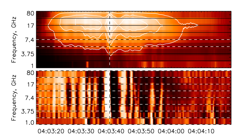
Figure 2: Top: Dynamic spectrum of the 10 March 2001 flare burst. The NoRP measurements are complemented by SRS measurements at 5.4 and 7.4 GHz. Contours: $2000\times(0.1,0.3,0.5,0.8)$ sfu. Bottom: The derivatives of the time profiles.

In the dynamic spectrum (Figure 2, top) the NoRP data are complemented by the SRS profiles at 5.4 GHz and 7.4 GHz to fill large gap between the NoRP receiving frequencies 3.75 GHz and 9.4 GHz. The shape of the microwave spectrum does not change much during the burst that is visualized by similarity of the contours of equal intensity shown in the dynamic spectrum (Figure 2, top). The time profiles in Figure 1 show a number of pulses besides the main peak. They are clearly seen in the time derivative of the dynamic spectrum (Figure 2, bottom).

Time derivative of dynamic spectrum (Figure 2, bottom) shows wide band fine structures during the entire bursts. Bright strips correspond to increase of the emission, while the dark ones show emission decrease. The duration of the shortest strips is comparable with the NoRP temporal resolution (0.1 s), and there bandwidth covers the entire spectral range from 1 GHz to 80 GHz in some cases. The strips are not noise or interference since they are wider than several frequency channels including data from different observatories. Note that most of the broadband pulses display no frequency drifts, although any drift value within $\pm 800$ GHz/s is measurable with given time resolution (0.1 s) and spectral bandwidth (80 GHz) of the pulses. The duration of decay phases (the dark strips after the bright ones) does not depend on the frequency.

At millisecond time scale there are pulses with reverse and normal frequency drift observed in the dynamic spectrum in interval within 04:03:37 – 04:03:56 UT, some of them are shown in Figure 4. The total bandwidth of the fine structures does not exceed 0.5 GHz and the life time is about 50 ms. The corresponding drift rates are within $10-15$ GHz/s in this event. The characteristic frequency of the fine structures rises from 4.5 GHz up to 7 GHz during this interval.

Time profiles of the hard X-ray emission are remarkably similar to the microwave profiles (Figure 3). The same profiles were observed with the Wide-Band Spectrometer at the high-energy band (80-600 keV). Note, that HXR emission is delayed relative to the radio emission. The overall L signal delays relative to various radio frequencies by about 1-2 s, although the delay between the impulsive peaks occurring at about 04:03:40 UT is shorter than 1 s. At higher energies the delays are shorter being a fraction of second. In particular, the cross correlation between the H channel and 35 GHz light curve yields the delay of 0.5 s with the correlation coefficient equal to $0.8$.

3.2 Spatial characteristics

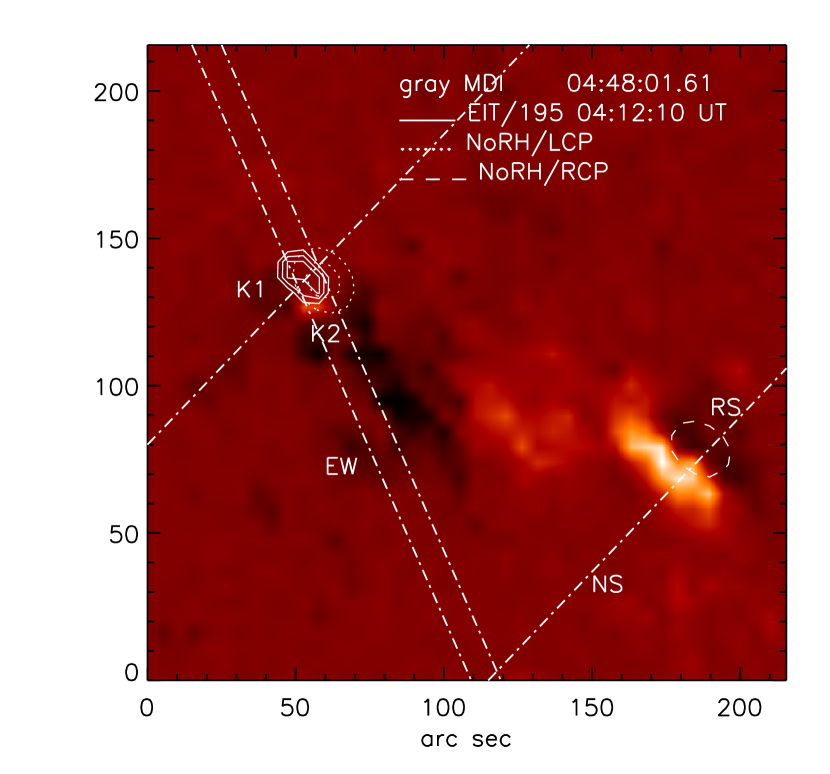
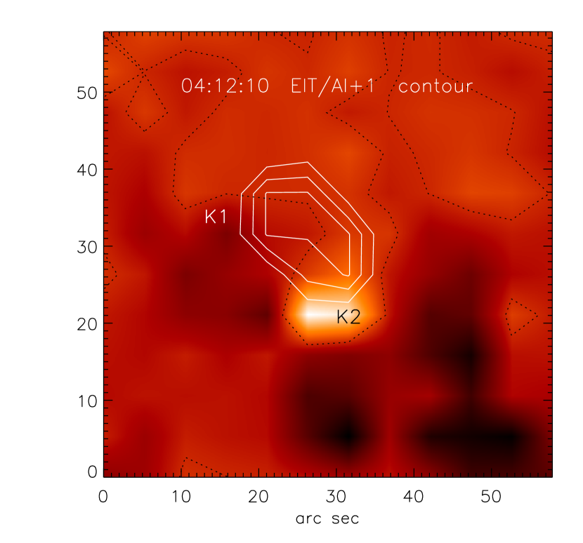
Figure 5: Left: Flare sources in UV and microwaves (right and left circular polarization). Dash-dotted lines show directions of the EW and NS fan strips. Right: Extended EIT partial frame with MDI magnetogram background. Dashed contour shows the magnetic neutral line.

The flare spatial structure in $H_{\alpha}$ emission was studied by Uddin et al. (2004) and Chandra et al. (2006). Before the flare, emerging flux of N polarity had penetrated into the S polarity region and triggered the flare. From the spatial correlation between different waveband sources it was concluded that the flare had the three-legged structure, i.e., it may be considered to be one of the typical configuration of loops as determined earlier by Hanaoka (1996). The $H_{\alpha}$ flare began (around 04:01 UT) as two bright kernels (K1 and K2), which rapidly transformed during the flare peak into a bright region expanding in the southwest direction. A short loop connecting magnetic regions of opposite polarity is seen in 195 Å emission (Figure 5); its length is about $10^{4}$ km. One more source (so called remote source, RS) appeared after 04:03:51 UT at 17 GHz. The RS was located 150 arcsec southwest from the main flare site (Figure 5) and had right handed polarization; the presence of the RS is confirmed by a secondary peak at 280 arc sec in the 5.7 GHz SSRT/NS scan at 04:04:21 UT (Figure 6, middle), which is unpolarized, however, at this relatively low frequency.

The footpoints of the loop are seen in the 17 GHz polarization images during the late decay phase of the burst (Figure 7, right panel). The shown maps are the result of averaging of the emission over more than a minute. The averaging is made since the brightness temperature of right handed emission was rather weak. In the main phase of the burst the bulk of microwave emission is generated in the source K2 with the north polarity of magnetic field, and it is left hand polarized. This means that the microwave source K2 is polarized in the ordinary wave mode. The magnetic field near the footpoints can be estimated from the MDI magnetogram as $-170$ G (K1) and 340 G (K2).

The spatial behavior of the HXT emission is studied by Chandra et al. (2006) in detail. In all energy bands only single source was observed. The estimated size of the HXR source was $7.0\times 3.8$, $6.7\times 3.3$, $6.5\times 3.3$ and $6.2\times 3.2$ arc sec in L, M1, M2, and H energy bands respectively. According to Figure  6 in Chandra et al. (2006) the HXR source is located near source K1. Note that the situation when the brightness peaks in the hard X-ray and the microwaves are located in the opposite ends of a single loop is typical for asymmetric magnetic loops.

The SSRT 1d images are shown in Figure 6. The vertical lines correspond to the integration paths crossing the centers of the two-dimensional brightness distribution at 17 GHz; these integration paths are shown by dash-dotted lines for both EW and NS linear arrays in Figure 5. The microwave source position did not change in the NS scans, while slightly shifts to the West in the EW scans at the burst peak. The sources K1 and K2 are not resolved in the SSRT scans. The size of the 5.7 GHz microwave source is about 50 arc sec in the NS scans and 25 arc sec in the EW scans. On the contrary the polarization distributions are radically changing with time. At the burst peak the polarization sense changes from the left handed to the right handed polarization and then back in the NS scans. In the EW scans a two-polarity structure appeared in the time interval around the burst peak.

3.3 Spectrum description

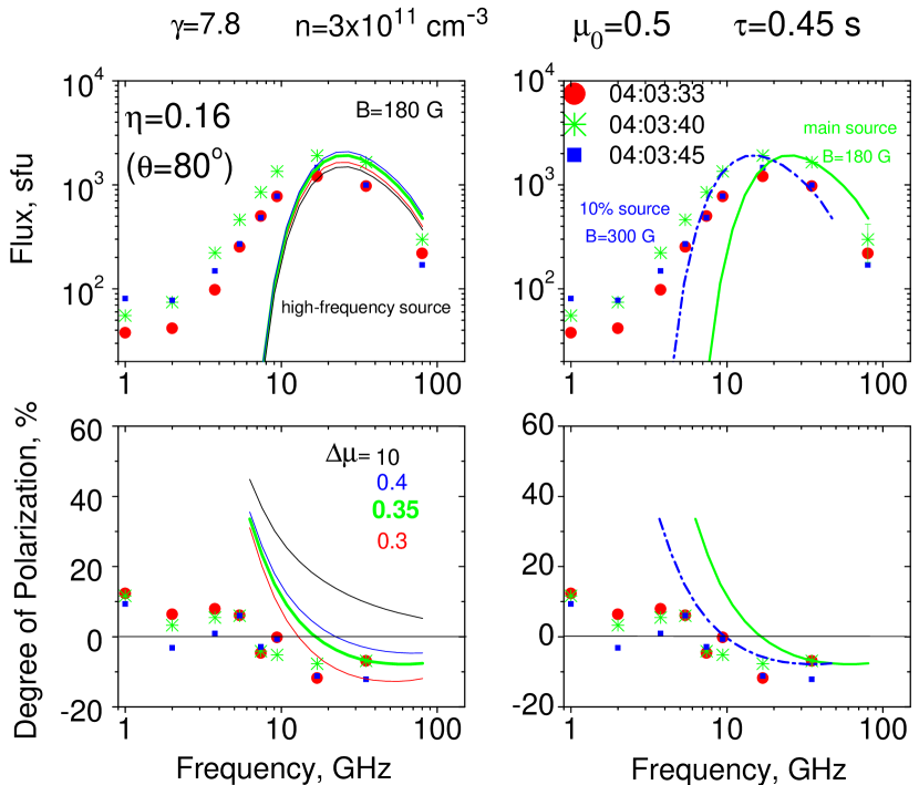
Figure 8: Observed spectra at various time frames (symbols) and fitting results (curves). Left column presents the best fit curves for the total intensity and degree of polarization for the high-frequency source, green/thick lines as well as curves obtained by small variations of the dispersion in the fast electron angular distribution (blue and red curves). Black curve show the results for the isotropic electron distribution all other conditions being equal. Right column displays the best fit curves for the high-frequency source (green/solid) supplemented by curves for the emission from a secondary source with higher magnetic field and smaller amount of the fast electrons (blue/dash-dotted curves) all other conditions being equal. This simple two-source model is good enough to describe the total intensity, although insufficient to fit the polarization data.

The microwave spectra are shown in Figure 8 at three moments corresponding to the main peak and neighboring peaks. The spectra are similar to each other. At low frequencies the spectra increase with index $\gamma\simeq 1.9$. Spectral peak is at about 17 GHz. At high frequencies the spectrum decreases rather quickly with the high-frequency spectral index $\gamma\simeq-2.1$.

The hard X-ray spectrum $I(E)$ was studied by Chandra et al. (2006) using the Yohkoh$\backslash$HXT data. At the peak time they obtained $I(E)=F_{o}E_{ph}^{-\gamma}=2.02\times 10^{5}E_{ph}^{-2.4}$ photons $\cdot$ cm${}^{-2}\cdot$ s${}^{-1}\cdot$ keV^-1. Assuming the electron spectrum in the form $F_{el}(E)=AE^{-\delta}$ electrons/s we get the parameters of electron flux under the thick-target assumption as follows, by making necessary corrections for the equation given by Brown (1971):

$$A=5.2\times 10^{33}\gamma^{2}(\gamma-1)^{2}B(\gamma-0.5,1.5)F_{o}=5.1\times 10^{39}$$ (1)

and $\delta=\gamma+1=3.4$, where $E$ is expressed in keV.

3.4 Summary of observations

Here we summarize main observational characteristics of the event important for further analysis:

1. The microwave emission in the 10 March 2001 event consists of many short broadband pulses.

2. Type III like features are observed around 5 GHz.

3. The microwave emission is O-mode polarized at 17 GHz.

4. The polarization at 5.7 GHz displays high variability and corresponds to X-mode at the peak time.

5. HXR light curves are remarkably similar to the microwave light curves.

6. HXR is delayed by a fraction of second compared with the microwave emission.

4 Model

4.1 General trends and model dependences

Our goal in the analysis of the microwave emission is to derive important source parameters from forward fitting of the observed radio spectra by the gyrosynchrotron formulae. However, as is widely known (e.g., Bastian et al., 2007) the gyrosynchrotron emission depends on too many physical effects and parameters even if angular distribution of fast electrons is isotropic. Expected presence of the beam-like anisotropy of fast electrons adds a few new free parameters, which complicates further the procedure of the fitting. Therefore, before developing a specific forward fitting model dealing with gyrosynchrotron emission produced by electron beams, we critically evaluate the observed properties of the burst to restrict or fix as many parameters as possible.

First of all, we make use of the close similarity of the radio and HXR light curves. This similarity suggests that no trapping effect is important for this event and both HXR and microwave emissions are produced by the same electron distribution. The peak injection rate of the electrons above 10 keV derived from the HXR spectrum is $J(>10~{}\rm keV)\simeq 8.5\cdot 10^{36}$ electrons/sec. We adopt that the total number of the emitting electrons in the radio source is $N_{\rm tot}=\tau_{l}J(>10~{}\rm keV)$, where $\tau_{l}$ is the characteristic life time of the emitting electrons in the radio source. Since no trapping is important, we adopt that $\tau_{l}$ is a single, energy-independent, free parameter, which will be determined later from the forward fitting model. It is clear, however, that $\tau_{l}$ must not exceed a few seconds, the typical duration of the single pulses composing the burst. Then, regarding the energy dependence of the electron distribution, we adopt the simplest assumption of a single power-law over the momentum modulus with the spectral index determined from the HXR spectrum (note, the energetic spectral index of 3.4 corresponds to the index of 7.8 in the distribution over momentum).

Second, address the question what can cause the delay of the HXRs relative to microwave emission. If the electron beam is injected somewhere at the top of the loop towards the foot points, then directly precipitating electrons will first produce the HXR and a fraction of the electrons reflected back into the loop will later produce the radio emission. Thus, the model involving directly precipitating beam predicts opposite delay (HXR leads radio) to what is actually observed. Note, that models with electron trapping also predict a delay of radio emission relative to HXR emission (Melnikov, 1994).

The only transport model allowing radio to lead HXR is a ’single reflection’ model, which is adopted below. Specifically, if a particle beam with some angular scatter is injected at a asymmetric magnetic trap towards a foot-point with stronger magnetic field, most of the electrons can be reflected back to form a hollow beam, produce gyrosynchrotron emission in the region of relatively strong magnetic field, and then after corresponding travel time over the loop reach the other foot point with weaker magnetic field to penetrate deeper into the chromosphere and produce HXRs. In this case the observed delay between radio and HXR originates naturally. In addition, the presence of initially downward injected beam is confirmed by the reverse drifting coherent subbursts (Figure 4) leading both microwave and HXR peaks by a fraction of second.

In our event the formation of a asymmetric loop is likely because the photospheric magnetic field has the extremes of $-170$ G and +340 G at the flare kernels K1 and K2 respectively. This means that the magnetic field in the radio source should belong to the range +170 G $<B<$ +340 G. Indeed, if the regions of weaker magnetic field provided noticeable radio emission, then the trapping of the particles between $-170$ G and 170 G loop layers were important, which is not observed.

Third, the information about the largest possible value of the magnetic field at the source allows to make a firm conclusion about possible role of the gyrosynchrotron self-absorption in the event. This question is important because the low-frequency slope of the spectrum ($\gamma=1.9$) is consistent with that expected for the optically thick gyrosynchtotron radiation (Dulk, 1985). However, with the given magnetic field range and the given electron distribution it is impossible to ensure the spectral peak at about 17 GHz (as observed) by the self-absorption effect unless the source is extremely compact, with the linear scale less than $700$ km. In this case, however, the number density of the fast electrons will exceed $10^{12}$ cm^-3, which we believe is not realistic. Thus, we adopted the typical angular scale of the source to be 6” consistent with imaging observations of the radio source.

Alternatively, a large value of the microwave spectral peak frequency can be provided by Razin effect, which requires high plasma density at the radio source. Indeed, the presence of high plasma density at the source is likely because we observe type III like drifting bursts around 5 GHz (Figure 4). Accordingly, we adopt the background plasma density to be

$$n_{e}=3\cdot 10^{11}{\rm cm}^{-3}.$$ (2)

This estimate agrees with the value of the emission measure determined from the soft X-ray emission (Uddin et al., 2004).

In such a dense plasma the Razin-effect is strong for the entire range of the magnetic field $170-340$ G. In conditions of strong Razin effect the low-frequency slope of the gyrosynchrotron spectrum in the uniform source is much steeper than one observed. We must, therefore, conclude that the low-frequency slope of the spectrum is eventually formed by the source inhomogeneity, i.e., by different layers with the magnetic field ranging from 170 G to 340 G in the region of kernel K2. In such a dense plasma the free-free absorption is typically important throughout the microwave range (Bastian et al., 2007). However, high plasma temperature of about 3$\cdot 10^{7}$K was determined for this event from the soft X-ray data (Uddin et al., 2004), therefore, the free-free optical depth is less than unity at $f>7$ GHz. Thus, we will not take into account the free-free absorption in our analysis.

We note that the spectral peak provided by the Razin effect increases as the magnetic field decreases. This means, in particular, that lower-frequency emission should arise lower in the loop, in contrast to usual situation when higher-frequency sources are located lower in the corona. We checked that the position of the brightness peak at 17 GHz is indeed displaced southwest by about 5” relative to the 34 GHz brightness peak in agreement with the prediction made. Therefore, the high-frequency emission should arise from the region of the lowest possible magnetic field, thus, we adopt

$$B=180~{}G$$ (3)

consistent with the requirement $B>170$ G. Now, when most of the source parameters are fixed based on straightforward use of various observational indicators, we can turn to formulating the forward fitting model.

4.2 Forward fitting scheme

Even though there are many individual measurements of the radio emission produced by the considered event, we can make use of only a minor fraction of them. Indeed, since the low-frequency part of the spectrum is related to the inhomogeneity of the source, which cannot be reliably constrained by the observations, we can only model the high-frequency part of the radio spectrum by the uniform source (which we refer to as ’high-frequency source’).

Specifically, we adopt that the high-frequency source is entirely responsible for the emission at 80 GHz and 35 GHz and for a significant fraction of the emission at 17 GHz. Therefore, we have at best five different observational data points (Stokes I and V at 17 GHz and 35 GHz and Stokes I at 80 GHz), which may allow for finding four free parameters or less. It is clear, that the weights of the measurements are different from each other: the highest weight is given to measurements at 35 GHz (5$\%$ error in the intensity, and 10$\%$ error in polarization) as they have a small experimental error and should be well described by the uniform source model. The 80 GHz intensity has lower weight (while it should be described by the uniform model even better that the 35 GHz data, the 80 GHz intensity is measured with 40$\%$ error). The experimental error at 17 GHz is small, however, the effect of source inhomogeneity becomes important. Thus, we adopt that the high-frequency source provides 70$\%$ of the observed flux at 17 GHz with error of 40$\%$; the error of 100$\%$ in the degree of polarization at 17 GHz is adopted.

In previous subsection we mentioned already that one of the free parameters we determine from the fitting is the characteristic life time $\tau_{l}$ of the emitting electrons at the radio source. Another important parameter, which is not known from the observations, is the viewing angle $\theta$ between the line of sight and the direction of the magnetic field at the source, so the viewing angle is the second free parameter in the forward fitting scheme. Thus, we have to use a test function for the angular part of the electron distribution, which depends on only one or two free parameters. Our model involving one reflection of the electrons from the magnetic mirror cannot be described by a function with a single free parameter: it must include both the direction where the angular distribution reaches the maximum, which differs from the direction along the field lines after the reflection, and typical angular scatter of the distribution. Thus, a test function with two free parameters is necessary. As a simplest approximation we adopt a normalized gaussian angular distribution over the cosine of the pitch-angle with unknown mean and dispersion:

$$f_{2}(\mu)\propto\exp\left(-{(\mu-\mu_{0})^{2}\over\Delta\mu^{2}}\right).$$ (4)

Then, we apply a nonlinear code that adjusts model free parameters to minimize the $\chi^{2}$ statistics using the downhill simplex method (Press et al., 1986). The $\chi^{2}$ statistics is calculated as

$$\chi^{2}=\sum_{i=1}^{N}{{(S_{i}^{obs}-S_{i}^{mod})^{2}}\over{\sigma_{i}^{2}}},$$ (5)

where $S_{i}^{obs}$ are the observational data of either Stokes I or V for the selected three frequencies, $\sigma_{i}$ are defined by the errors introduced above, $S_{i}^{mod}$ are the model values of the intensity and polarization.

Our current forward fitting scheme is different from the scheme applied previously (Bastian et al., 2007) in two instances. First of all, minimizing the $\chi^{2}$ statistics we employ both intensity and polarization data simultaneously in the same run, which is the first example when the polarization data is used for quantitative diagnostics of the fast electron distribution. And then, our model function is the exact expression of the gyrosynchrotron emission including the summation over the series of the Bessel functions and their derivatives. Because the magnetic field at the source is somewhat low, the contribution of large harmonics is important at high frequencies, therefore, we had to use the sum over 1600 terms of the series to describe the emission correctly up to 80 GHz. This made our scheme computationally expensive: the full run with one spectrum took about 50 hours of the PC with 2.1 GHz processor.

4.3 Forward fitting results

Given that the observed spectrum does not evolve much during the burst, while the forward fitting scheme employing exact gyrosynchrotron equations is very time consuming, we concentrated on study of the emission at the peak time of the burst (04:03:40 UT) only. Result of the fitting is shown in Figure 8. A number of important things should be noticed in the figure. First, the model radio spectra (top left panel) obtained for the electron energy spectrum derived from HXR data are good match for the observed high-frequency part of the radio spectra. Thus, the data is consistent with the model assumption of a single power-law electron spectrum in the event. Second, the curves for the degree of polarization are very sensitive to the details of the electron angular distribution. In particular, the polarization data is entirely inconsistent with isotropic angular distribution of the fast electrons, since the isotropic distribution would produce X-mode polarized emission, while the observed polarization corresponds to O-mode emission. The gyrosynchrotron radiation produced by oblique beam observed by quasitransverse direction is O-mode polarized as needed. The exact value of the degree of polarization depends strongly on the details of the pitch-angle distribution, thus, the joint use of the intensity and polarization measurements is indeed a key to constrain the angular distribution of the electron beam. For the peak time of the burst the following parameters provide the best fit to the observed spectrum and polarization:

$$\tau_{l}=0.45~{}s,\qquad\theta=80^{o},\qquad\mu_{0}=0.5,\qquad\Delta\mu=0.35.$$ (6)

All these numbers look reasonable against observations and theory of gyrosynchrotron radiation from anisotropic electron distribution. Indeed, the life-time of the fast electrons is small enough, $\tau_{l}\approx 0.45$ s, i.e., less than the radio peak duration as required. Then, as is known from the gyrosynchrotron theory, the O-mode polarization of the optically thin source is only possible for beam-like electron distributions and for viewing angles larger than the peak angle in the pitch-angle distribution. The obtained values of $\theta$ and $\mu_{0}$ obey these requirements since $\cos\theta=0.16<\mu_{0}$.

It is tempting now to subtract the model contribution of the high-frequency source from the observational data points and repeat the forward fitting procedure. Indeed, we can perform a reasonable fit to the total power data. As an example, a contribution of a ”lower-frequency source” with the same pitch-angle distribution but with stronger magnetic field ($B\approx 300$ G), while smaller life-time of the fast electrons ($\tau_{l}\approx 0.05$ s) is shown in the figure.

However, it is not possible to perform a consistent fit to the polarization measurements, which is the key to constrain the electron angular distribution, because the observed degree of polarization is essentially the result of averaging of various contributions along the non-uniform source. This conclusion is in agreement with high spatial and temporal variability of the polarization patterns observed at 5.7 GHz, which is most probably a result of changing relative contributions from different parts of an inhomogeneous source (note a very strong frequency dependence of the degree of polarization in the model curves below 10 GHz in Figure 8). Therefore, the low-frequency observations cannot be conclusively fitted by the uniform source model.

5 Discussion

In this paper we presented a new tool of studying electron beams accelerated during solar flares by analysis of the gyrosynchrotron emission produced by the beams. Methodologically, this result is achieved by quantitative use of the polarization measurements of the microwave gyrosynchrotron emission. Specifically, to obtain the information of the beam-like angular distribution of the accelerated electrons we developed a nonlinear $\chi^{2}$ fit employing Stokes I $\&$ V measurements simultaneously and exact gyrosynchrotron formulae.

This approach allows for unambiguous detection of oblique beams at the radio source. In addition, our scheme yields a number of important physical parameters of the radio burst such as the viewing angle of the radio emission relative to the magnetic field at the source, characteristic parameters of the electron distribution over pitch-angle, and typical life time of the electrons in the radio source, see Eq. (6).

The diagnostics of the electron beam obtained from the fit of the gyrosynchrotron data within ’one-reflection model’ is consistent with all other available observations. In particular, the time delays of the hard X-rays relative to the microwaves (a fraction of second) is consistent with the transit time of the electrons with relatively large pitch-angles (found from the forward fitting technique) through the flaring loop of about 10⁴ km in projection. In addition, the fine structures consisted of the reverse drift bursts followed by the normal drift bursts detected at about 5 GHz are in agreement with the ’one-reflection model’, which implies the downward beam propagation followed by its reflection at the magnetic mirror and consequent upward motion of the beam. The radio data suggest that the main radio source is filled by a rather dense plasma, Eq. (2), with the plasma frequency of about 5 GHz. The radio emission observed at lower frequencies (3.75 and 2 GHz) cannot be produced at this main source. The most straightforward interpretation for this low-frequency component is to postulate an adjacent more tenuous loop, where a minor fraction of the accelerated electrons produce lower-frequency radiation. Such a larger loop is likely and confirmed by the presence of a remote source magnetically connected with the main flare site. If so, larger decay constant and the observed delay of the low-frequency emission relative to higher-frequency emission (see §3.1) receives a natural interpretation because it simply relates to larger source size implying longer transit time, where, in addition, some trapping of the electrons can be important.

Another possible effect of the dense plasma is an enhanced role of the Coulomb collisions on the radiating electrons. Given relatively low value of the magnetic field at the source, it is easy to estimate the typical energies of the radio emitting electrons as $1-10$ MeV, which have the Coulomb energy decay time $\tau_{c}>15$ s, which is much longer than the transit time. The time of isotropization of these relativistic electrons due to Coulomb collisions is even longer than the energy decay time (Petrosian, 1985). We, thus, conclude that the Coulomb collisions have very little effect on the electron distribution at the time scale of the electron precipitation ($\sim 1$ s) in this event.

Although we quantitatively describe the emission at the burst peak only, we can reliably extrapolate the main findings, such as acceleration of the fast electrons in the form of beams and the one-reflection transport model to the entire burst duration. It follows from the close similarity between the radio and the hard X-ray light curves and from the constancy of the sense of polarization in the main source at 17 GHz. This means that some of the flares, such as one considered here, can predominantly accelerate electrons along the magnetic field lines even though the pitch-angle distribution of the beams has some angular scatter.

The potentiality of the developed method is very strong and will be especially helpful when imaging spectroscopy data is availably. However, the routine use of this method requires optimization of the computation scheme, which is not fast enough at present. Therefore, deducing simplified, although precise enough, gyrosynchrotron formulae for anisotropic electron distributions can be very helpful here.

6 Conclusion

Electron beams with some angular scatter can efficiently produce microwave continuum bursts via gyrosynchrotron mechanism. As was shown theoretically by Fleishman and Melnikov (2003), the gyrosynchrotron emission produced by electron beams can be distinguished from that produced by isotropic electron populations by analysis of the degree of polarization of the microwave emission. Here we presented a compelling example of such event, where the optically thin gyrosynchrotron radiation is indeed O-mode polarized as expected for the beam-like distributions. Remarkably, the presence of the beam is confirmed by the whole set of the available data for this event.

In case of the radio data with good enough quality (including both intensity and polarization) the use of forward fitting inversion methods allows for quantitative diagnostics of the fast electron angular distribution as well as a number of other important physical parameters of the flaring source. These methods will become much more useful when the imaging spectroscopy data is available.

Figure 1: Microwave fluxes, recorded by the NoRP polarimeters. Left: total intensity (R+L), right: polarized intensity (R-L). Magnitudes of fluxes are in sfu.

Figure 3: Radio vs Yohkoh/HXT light curves. Energy ranges are L(14 – 23 keV), M1(23 – 33 keV), M2(33 — 53 keV), H(53 – 93 keV). HXR light curves (dashed) are normalized such as to match the peak value of the corresponding radio light curves (solid). Available at $http://gedas22.stelab.nagoya-u.ac.jp/HXT/catalogue/image\_html/eid\_html/eid\_25110.html$

Figure 4: Drifting fine structures recorded slightly before the main flare peak with the PMO spectrometer.

Figure 6: One-dimensional brightness distributions (scans) recorded with the EW and NS arrays at 5.7 GHz in intensity (left) and polarization (right). Each point in these brightness distributions is a result of integration of the true brightness along a line parallel to the dash-dotted EW (EW-scans) or NS (NS-scans) lines shown in Figure 5. Solid profiles correspond to the burst peak. Profile magnitudes are in arbitrary units. Vertical dash-dotted lines correspond to positions marked in the NoRH map in Figure 5 (left). Middle panels show the appearance of the unpolarized RS in the NS scans.

Figure 7: Brightness distributions in intensity and polarization at 17 GHz. Average values of contours are $4\times 10^{7}$ K in intensity, $1.5\times 10^{4}$ K in right handed polarization, and $-6\times 10^{6}$ K in left handed polarization in the left panel, and $2\times 10^{6}$ K in intensity, $1.35\times 10^{4}$ K in right handed polarization, and $-10^{5}$ K in the right panel.

References

- Altyntsev et al. (2007) Altyntsev, A. T., Grechnev, V. V., Meshalkina, N. S., & Yan, Y. 2007, Sol. Phys., 242, 111
- Aschwanden (2002) Aschwanden, M. J. 2002, Particle Acceleration and Kinematics in Solar Flares (Dordrecht: Kluwer)
- Aschwanden (2005) Aschwanden, M. J. 2005, Physics of the Solar Corona. An Introduction with Problems and Solutions (New York: Springer)
- Bastian (2006) Bastian, T. B. ’Solar Physics with the Nobeyama Radioheliograph’, Proceedings of Nobeyama Symposium 2004, held in Kiyosato, Japan, October 26-29, 2004, Nobeyama Solar Radio Observatory, 2006, pp.1-8
- Bastian, Benz & Gary (1998) Bastian, T. S., Benz, A. O., & Gary, D. E. 1998, ARA&A, 36, 131
- Bastian et al. (2007) Bastian, T. S., Fleishman, G. D., & Gary, D. E. 2007, ApJ, 666, 1256
- Benka & Holman (1992) Benka, S. G., & Holman, G. D. 1992, ApJ, 391, 854
- Bianda et al. (2005) Bianda, M., Benz, A. O., Stenflo, J. O., Kuveler, G.,& Ramelli, R. 2005, A&A, 434, 1183
- Brown (1971) Brown, J. C. 1971, Sol. Phys., 18, 489
- Chandra et al. (2006) Chandra, R., Jain, R., Uddin, W., Shimura, K., Kosugi, T., Sakao, N., Joshi, A., & Despandey, M. R. 2006, Sol. Phys., 239, 239
- Ding (2003) Ding, M. D. 2003, Journal of the Korean Astronomical Society, 36, 49
- Ding et al. (2003) Ding, M. D., Liu, Y., Yeh, C.-T. & Li, P. I. 2003, A&A, 403, 1151
- Dulk (1985) Dulk, G. A. 1985, ARA&A, 23, 169
- Dulk & Mursh (1982) Dulk, G. A. & Mursh, K. A. 1982, ApJ, 259, 350
- Eidman (1958) Eidman, V. Ya. 1958, Sov. Phys. JETP, 7, 91
- Eidman (1959) Eidman, V. Ya. 1959, Sov. Phys. JETP, 9, 947
- Farnik & Karlicky (2007) Farnik & Karlicky, 2007, Sol. Phys., 240, 121
- Fleishman (2006) Fleishman, G. D. ’Solar Physics with the Nobeyama Radioheliograph’, Proceedings of Nobeyama Symposium 2004, held in Kiyosato, Japan, October 26-29, 2004, Nobeyama Solar Radio Observatory, 2006, pp.51-62
- Fleishman et al. (2007) Fleishman, G. D., Bastin, T. S., & Gary, D. E. 2007, ApJ, to be submitted
- Fleishman et al. (2003) Fleishman, G. D., Gary, D. E., & Nita, G. M. 2003, ApJ, 593, 571
- Fleishman and Melnikov (2003) Fleishman G. D. & Melnikov V. F. 2003, ApJ, 587, 823
- Fu et al. (2004) Fu, Q., Ji, H., Qin, Z., Xu, Z., Xia, Z., Wu, H., Liu, Y., Yan, Y., Huang, G., Chen, Z., Jin, Z., Yao, Q., Cheng, C., Xu, F., Wang, M., Pei, L., Chen, S., Yang, G., Tan, C., Shi, S. 2004, Sol. Phys., 222, 167
- Gary (2006) Gary, D. E. ’Solar Physics with the Nobeyama Radioheliograph’, Proceedings of Nobeyama Symposium 2004, held in Kiyosato, Japan, October 26-29, 2004, Nobeyama Solar Radio Observatory, 2006, pp.119-129
- Getmantsev (1952) Getmantsev, G. G. 1952, DAN SSSR, 83, 557
- Ginzburg (1951) Ginzburg, V. L. 1951, DAN SSSR, 76, 377
- Ginzburg (1953) Ginzburg, V. L. 1953, Uspekhi Fiz. Nauk, 51, 343
- Ginzburg and Syrovatsky (1964) Ginzburg, V. L., & Syrovatsky, S. I. 1964, The Origin of Cosmic Rays (New York: Macmillan Co.)
- Grechnev et al. (2003) Grechnev, V. V. Lesovoi, S. V., Smolkov, G. Ya., Krissinel, B. B., Zandanov, V. G., Altyntsev, A. T., Kardapolova, N. N., Sergeev, R. Y., Uralov, A. M., Maksimov, V. P., & Lubyshev, B. I. 2003, Sol. Phys., 216, 239
- Henoux et al. (2003) Henoux, J. C., Vogt, E., Sahal-Brechot, S., Karlichky, M., Feautrier, N., Fa’rni’k, F., Chambe, G., Balanca, C. 2003, ASP Conf. Proc., 307, 480
- Klein (1987) Klein, K.-L. 1987, A&A, 183, 341
- Korchak and Terletsky (1952) Korchak, A. A. and Terletsky, Ya. P. 1952, Zh. Eks. Teor. Phys., 22, 507
- Korchak (1957) Korchak, A. A. 1957, Soviet Astronomy, 1, 360
- Kundu et al. (2001) Kundu, M. R., White, S. M., Shibasaki, K., Sakurai, T., & Grechnev, V. V. 2001, ApJ, 547, 1090
- Lui, Ding&Fang (2001) Liu, Y., Ding, M. D. and Fang, C. 2001, ApJ, 563, L169
- Melnikov (1994) Melnikov, V. F. 1994, Radiophysics and Quantum Electronics, 37, 557
- Melnikov et al. (2002a) Melnikov, V. F., Shibasaki, K., & Reznikova, V. E. 2002a, ApJ, 580, L185
- Melnikov (2006) Melnikov, V. F. ’Solar Physics with the Nobeyama Radioheliograph’, Proceedings of Nobeyama Symposium 2004, held in Kiyosato, Japan, October 26-29, 2004, Nobeyama Solar Radio Observatory, 2006, pp.9-20
- Nakajima et al. (1985) Nakajima, H., Sekiguchi, H., Sawa, M., Kai, K., & Kawashima, S. 1985, PASJ, 37, 163
- Nakajima et al. (1994) Nakajima, H., Nishio, M., Enome, S., Shibasaki, K., Takano, T., Hanaoka, Y., Torii, C., Sekiguchi, H., Bushimata, T., Kawashima, S., Shinohara, N., Irimajiri, Y., Koshiishi, H., Kosugi, T., Shiomi, Y., Sawa, M., & Kai, K. 1994, Proc. of the IEEE, 82, 705
- Nindos (2006) Nindos, A. ’Solar Physics with the Nobeyama Radioheliograph’, Proceedings of Nobeyama Symposium 2004, held in Kiyosato, Japan, October 26-29, 2004, Nobeyama Solar Radio Observatory, 2006, pp.37-48
- Nindos et al. (2000) Nindos, A., White, S. M., Kundu, M. R., & Gary, D. E. 2000, ApJ, 533, 1053
- Petrosian (1981) Petrosian, V. 1981, ApJ, 251, 727
- Petrosian (1985) Petrosian, V. 1985, ApJ, 299, 987
- Press et al. (1986) Press, W. H., Flannery, B. P., & Teukolsky, S. A. 1986, Numerical Recipes: The Art of Scientific Computing (Cambridge: Univ. Press)
- Ramaty (1969) Ramaty, R. 1969, ApJ, 158, 753
- Ramaty & Petrosian (1972) Ramaty, R., & Petrosian, V. 1972, ApJ, 178, 241
- Ramaty et al. (1994) Ramaty, R., Schwartz, R. A., Enome, S., & Nakajima, H. 1994, ApJ, 436, 941
- Smolkov et al. (1986) Smolkov, G. Ia., Pistolkors, A. A., Treskov, T. A., Krissinel, B. B., & Putilov, V. A. 1986, Ap&SS, 119, 1
- Torii et al. (1979) Torii, C., Tsukiji, Y., Kobayashi, S., Yoshimi, N., Tanaka, H., & Enome, S. 1979, Proc. of the Res. Ist. of Atmospherics, Nagoya Univ., 26, 129
- Trottet et al. (2002) Trottet, G., Raulin, J.-P., Kaufmann, P., Siarkowski, M., Klein, K.-L., & Gary, D. E. 2002, A&A, 381, 694
- Uddin et al. (2004) Uddin, W., Jain, R., Yoshimura, K., Chandra, R., Sakao, T., Kosugi, T., Joshi, A., & Despande, M. R. 2004, Sol. Phys., 225, 325
- Veronig & Brown (2004) Veronig, A. M., & Brown, J. C. 2004, ApJ, 603, L117
- Yoshimori et al. (1992) Yoshimori, M., Takai, Y., Morimoto, K., Suga, K., Ohki, K., Watanabe, T., Yamagami, T., Kondo, I., & Nishimura, J. 1992, PASJ, 44, L51
- Zhou, Huang & Wang (1999) Zhou, A.-H., Huang, G.-L. & Wang, X.-D. 1999, Sol. Phys., 189, 345