RHESSI Microflare Statistics II.
X-ray Imaging, Spectroscopy & Energy Distributions.

Abstract

We present X-ray imaging and spectral analysis of all microflares the Reuven Ramaty High Energy Solar Spectroscopic Imager (RHESSI) observed between March 2002 and March 2007, a total of 25,705 events. These microflares are small flares, from low GOES C Class to below A Class (background subtracted) and are associated with active regions. They were found by searching the 6-12 keV energy range during periods when the full sensitivity of RHESSI’s detectors was available (see paper I). Each microflare is automatically analyzed at the peak time of the 6-12 keV emission: the thermal source size is found by forward-fitting the complex visibilities for 4-8 keV, and the spectral parameters (temperature, emission measure, power-law index) are found by forward fitting a thermal plus non-thermal model. The combination of these parameters allows us to present the first statistical analysis of the thermal and non-thermal energy at the peak times of microflares. On average a RHESSI microflare has a fitted thermal loop width 8 Mm (11^′′), length 23 Mm (32^′′) and volume $1\times 10^{27}$ cm³, temperature 13 MK, emission measure $3\times 10^{46}$ cm^-3 and density of $6\times 10^{9}$ cm^-3. There is no correlation between the loop size and the flare magnitude, either flux in the loop or GOES class, indicating that microflares are not necessarily spatially small. There is also no clear correlation between the thermal parameters except between the RHESSI and GOES emission measures, the GOES values are generally twice the RHESSI emission measures. The microflare thermal energy at the time of peak emission in 6-12 keV ranges over $10^{26}$ to $10^{30}$ erg and has a median value of $10^{28}$ erg. The frequency distribution of the thermal energy deviates from a power-law at low and high energies arising from a deficiency of events due to instrumental and selection effects. It is difficult to compare this energy distribution to previous thermal energy distributions of transient events, as the work sought nanoflares through imaging in EUV or soft X-rays and covered just a few hours. There are large uncertainties in the majority of the non-thermal parameters, due to the steep spectra down to low energies. We typically find a power-law index of $7$ above a break energy of $9$ keV, which corresponds to a low-energy cut-off in the electron distribution as low as $12$ keV. The resulting non-thermal power estimates, covering $10^{25}$ to $10^{28}$ erg s^-1 with median value of $10^{26}$ erg s^-1, therefore have large uncertainties as well. The few microflares with unexpectedly large non-thermal powers $10^{28}$ erg s^-1 have the smallest uncertainties, of about $10\%$. The total non-thermal energy however is still small compared to that of large flares as it occurs for shorter durations.

1. Introduction

The solar corona exhibits a myriad of transient energy releases over many scales, from large flares down to nanoflares. The frequency distribution of the energy in these events has been studied extensively (Crosby et al., 1993; Shimizu, 1995; Krucker & Benz, 1998; Aschwanden et al., 2000; Parnell & Jupp, 2000; Lin et al., 2001; Aschwanden & Parnell, 2002; Benz & Krucker, 2002) and has been found to be well represented by a power-law of the form

$$\mathrm{d}N=AW^{-\alpha}\mathrm{d}W$$ (1)

where $\mathrm{d}N$ is the number of events per unit time with energy between $W$ and $W+\mathrm{d}W$. These distributions are of particular interest as they elucidate the amount of energy available, how often it is released and in which events and form (thermal or non-thermal) it predominantly occurs. The energy release observed in normal-size flares is not sufficient to constantly and consistently heat the corona to the observed few million Kelvin. So the question is then whether this could be achieved by extending the observed flare-like energy releases to smaller scales. This concept can be expressed in terms of the power-law index of this distribution: if $\alpha\geq 2$ then the smallest events have a high occurrence rate and their energy dominates over larger flares, possibly matching the energy in coronal heating (Hudson, 1991). This requires the assumption that these distributions be continuous into the unobservable low-energy range, which is difficult to determine as there are instrumental and selection effects that both cut-off and bias the observed distribution (Aschwanden & Parnell, 2002).

The instantaneous thermal energy in these events may be calculated from

$$W_{\mathrm{T}}=3n_{\mathrm{e}}k_{\mathrm{B}}TV$$ (2)

where $n_{\mathrm{e}}$ is the electron density, $V$ the volume of the emitting thermal plasma, $k_{\mathrm{B}}$ Boltzmann’s constant, and $T$ the temperature. An estimate of the volume can be obtained by imaging the events, however there can be an overestimate in this observed volume to the true volume by a filling factor $f\approx 1$ to $10^{-4}$ (Cargill & Klimchuk, 1997; Takahashi & Watanabe, 2000). In this work we assume $f=1$, which will be discussed later. The temperature and emission measure may be found either directly from the spectrum or by imaging with different wavelength filters. Assuming constant density, the emission measure is related to the density and volume as $EM=n_{\mathrm{e}}^{2}V$ and so the thermal energy is

$$W_{\mathrm{T}}=3\sqrt{EM\cdot\,V}k_{\mathrm{B}}T.$$ (3)

Note that as losses are not taken into account here, the energy going into the thermal plasma will be larger. For the smallest events this thermal energy has been found using pixelated detectors in EUV and soft X-rays, with simultaneous pixel brightenings within some area being registered as an event (Shimizu, 1995; Krucker & Benz, 1998; Aschwanden et al., 2000; Parnell & Jupp, 2000; Aschwanden & Parnell, 2002; Benz & Krucker, 2002). The area inferred from these, often spatially discontinuous, brightened pixels gives an estimate of the volume, and observations using different filters give temperature and emission measure information.

The events observed in EUV are termed “nano”-flares as they have about $10^{-9}$ times the energy in large flares, the limit of their observability being down to $10^{24}$ erg (Aschwanden et al., 2000). Parker’s hypothetical nanoflare (Parker, 1988) is an estimate of the basic unit of a localized impulsive burst of energy release, with energies $<10^{24}$ erg, with ensembles of them constituting the observed events. The thermal energy of these events outside of active regions has been investigated in soft X-rays with Yohkoh/SXT (Krucker et al., 1997) finding energies of $10^{25}$ erg per event, and in EUV using SOHO/EIT (Krucker & Benz, 1998; Benz & Krucker, 2002) and TRACE (Parnell & Jupp, 2000; Aschwanden et al., 2000) providing energies between $10^{24}$ to $10^{27}$ erg. Small events in active regions, termed “active region transient brightenings”, were seen in soft X-rays with Yohkoh/SXT (Shimizu, 1995), with energies between $10^{26}$ to $10^{29}$ erg. All of these studies found the power law index of the frequency distributions to be between $\alpha=1.5-2.6$. Aschwanden & Parnell (2002) investigated the effect of instrumental bias on the different indices from SOHO/EIT, TRACE and Yohkoh/SXT data. Parnell (2004) later pointed out that the discrepancy between power-law indices from different instruments can be due to the effects of least-squares fitting some the of binned histograms. Similar indices were obtained when a maximum likelihood method (Parnell & Jupp, 2000) was used instead.

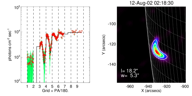
Figure 1.— (Left) Visibility forward fit model loop shape (solid line) onto the 4-8 keV visibilities amplitudes (diamonds with error bars) as a function of the phase for each grid. The amplitudes for each grid/subcollimator are shown between the dashed vertical lines, indicating the amplitudes measured as the grids rotate from a position angle of $0^{\circ}$ to $180^{\circ}$. Thus an amplitude measured in subcollimator 3 when rotated to a position angle of $45^{\circ}$ would be plotted against 3.25 on the x-axis. (Right) Resulting image of the visibilities shown in left panel, background image found using MEM NJIT algorithm (Schmahl et al., 2007), overplotted contours (25 %, 50 % and 75 %) representing the model shape. The loop length $l$ and width $w$ are quoted. Color version available in electronic edition.

The non-thermal hard X-ray emission is assumed to be due to a power-law distribution of electrons emitting hard X-rays via bremsstrahlung in a thick target. The resulting power-law photon spectrum reflects this electron distribution (Brown, 1971) allowing the power in these accelerated electrons above a low-energy cut-off $E_{\mathrm{C}}$ (in keV), to be calculated as

$$P_{\mathrm{N}}(\geq E_{\mathrm{C}}) = 9.5\times 10^{24}\gamma^{2}(\gamma-1)$$ (4)

$$\times\beta\left(\gamma-\text@frac{1}{2},\text@frac{3}{2}\right)I_{\mathrm{0}}E_{\mathrm{C}}^{(1-\gamma)}\quad\mathrm{erg~{}s}^{-1}$$

where $\gamma$ and $I_{\mathrm{0}}$ are the index and normalization of the photon power-law spectrum (in units of photon flux, s^-1 cm^-2 keV^-1) and $\beta(m,n)$ is the beta function (Brown, 1971; Lin, 1974). Therefore observing the hard X-ray spectrum of these events for various time intervals during each flare is sufficient to obtain an estimate of the non-thermal energy. However there is ambiguity in the low-energy cut-off, $E_{\mathrm{C}}$, because the observed photon spectrum depends only weakly on it, with a resulting flattening of the photon spectrum below $\epsilon_{\mathrm{B}}$ not uniquely related to $E_{\mathrm{C}}$, with $\epsilon_{\mathrm{B}}\leq E_{\mathrm{C}}$ (Holman, 2003). Uncertainty in $E_{\mathrm{C}}$ results in a larger uncertainty in the power estimate: a factor of 2 increase/decrease in $E_{\mathrm{C}}$ would result in a factor of 8 decrease/increase in the power for flat spectra ($\gamma=4$) or a factor of 64 decrease/increase in the power for steep spectra ($\gamma=7$).

Previous statistical studies of the non-thermal energy in flares used the energy threshold of the instrument as an estimate of $E_{\mathrm{C}}$, as they did not observe to low enough energies nor had sufficient energy resolution to observe the flattening of the spectrum. Crosby et al. (1993) using SMM/HXRBS estimated the non-thermal energy in large flares $>25$ keV, finding that the power distribution at the peak time of emission had a power-law with $\alpha=1.67$ over $10^{27}$ to $10^{30}$ erg s^-1 and the total non-thermal energy of these events had $\alpha=1.53$ over $10^{27}$ to $10^{32}$ erg. Microflares were observed down to 8 keV with CGRO/BATSE (Lin et al., 2001), finding energies over $10^{27}$ to $10^{30}$ erg, and by WATCH/GRANAT down to 10 keV (Crosby et al., 1998).

The Reuven Ramaty High Energy Solar Spectroscopic Imager RHESSI (Lin et al., 2002) is uniquely suited to investigate both the energy in the heated and accelerated electron populations, thermal and non-thermal emission, of these small events. This is due to its unprecedented sensitivity to 3-25 keV X-rays, high spectral resolution and imaging capabilities (Krucker et al., 2002). Previous studies of RHESSI microflares have concentrated on individual events (Krucker et al., 2002; Benz & Grigis, 2002, 2003) or small samples, often compared to other wavelengths, (Liu et al., 2004; Qiu et al., 2004; Battaglia et al., 2005; Kundu et al., 2005, 2006; Stoiser et al., 2007).

Here we present the first analysis of all RHESSI microflares found as transient bursts in 6-12 keV during periods of shutter-out observations, as detailed in part I of this article (Christe et al., 2008). Between March 2002 and March 2007 25,705 events were found. These are active-region phenomena of low C GOES class to below A-class. For the analysis presented here we measure the energy for 16 seconds around the time of peak emission in 6-12 keV. The peak time is only used as it presents the best opportunity to obtain enough counts above background to permit analysis in each event. Given the standard flare time profile of a sharp impulsive rise followed by slower decay phase, this means that this analysis will mainly cover the impulsive phase of these microflares.

The calculation of the thermal energy using equation (3) requires knowledge of the volume of the thermal source and thermal parameters from the spectrum. Imaging these events, and hence estimating the volume of thermal emission, is detailed in §2. In §3 the spectral fitting of the events is described, obtaining the thermal and non-thermal parameters of these events. The relationship between these parameters and those found using GOES data are discussed in §3.3. The calculation of the thermal energy and power in non-thermal electrons and the resulting frequency distributions is presented in §4. We discuss these results further, including how this analysis at peak time relates to the emission over the whole of the microflare, in §5.

2. Imaging Using Visibilities

RHESSI imaging is achieved through a Fourier-based method using rotation modulation collimators (RMCs) (Hurford et al., 2002). Each RMC time-modulates sources whose size scale is smaller than its resolution. This spatial information encoded in the time-modulation profile is normally reconstructed into an image via techniques such as back projection (Hurford et al., 2002).

A recently implemented alternative technique converts the time-modulation profile to complex visibilities before recovering the spatial information (Hurford et al., 2005). Each RHESSI visibility is a calibrated measurement of a single Fourier component of the source distribution measured at a specific spatial frequency, energy and time range. The visibilities are the complex quantities obtained from the fitted amplitude and phase of the modulated time profile for a particular roll orientation (rotational phase) of an individual RMC. The resulting set of visibilities for all roll angles and RMCs is a calibrated and compact representation of the original time profile, with little loss of information.

The advantage of using visibilities is twofold. First, as a smaller data set has to be processed, the image reconstruction from the visibilities is considerably quicker than using the time profile directly. Second, the visibilities are fully calibrated measurements, representing an intermediate step between the modulation profile and imaging, meaning that spatial information can be found directly from the visibilities without having to compute an image. This has been implemented in a Visibility Forward Fit (VFF) algorithm (Hurford et al., 2005) which determines the best-fit parameters, with statistical errors, for simple assumed source geometries (elliptical Gaussian, curved elliptical Gaussian, multiple sources etc).

We are primarily interested in the size of the thermal source, in order to make an estimate of the density and hence thermal energy, see §4. The images of thermal sources in microflares are taken over 4-8 keV and generally have a single elliptical source or loop shape. We fit a 2D model of a curved elliptical Gaussian to the 4-8 keV visibilities for 16 secs about the peak in 6-12 keV for each microflare. This attempts to fit a Gaussian profile along the curved semi-major axis, equivalent to the loop arc length. If the source is not appreciably curved an elliptical geometry of zero curvature is returned. Seven parameters are obtained from each fit of this 2D model: the centroid position (x,y), photon flux, FWHM loop length and width, curvature and position angle of the semi-major.

An example of this fitting is shown in Figure 1. Here in the left panel we have the visibility amplitudes, with statistical errors, for each grid and is position angle. The solid line is the VFF model loop shape which has fitted subcollimators 3,4,5,6,8 and 9 well. For this event the finest subcollimator, 1, is dominated by noise and so has little influence on the fit. Subcollimators 2 and 7 are not included as they provide a poor response in this energy range. The right panel shows the resulting image of these visibilities, produced using the MEM NJIT algorithm (Schmahl et al., 2007), with the VFF model loop from the left panel overplotted as contours. The contours correspond well with the background image. Further examples of the resulting fits are shown in Figure 2, again calculated using detectors 1,3,4,5,6,8 and 9.

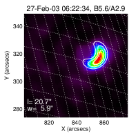
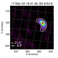
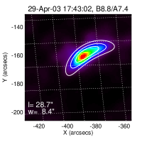
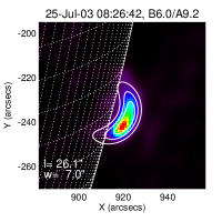
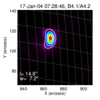
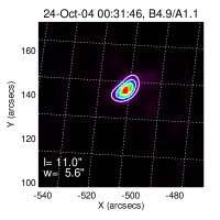
Figure 2.— Example microflares showing the MEM NJIT image (background) and the forward fit model shape (foreground contours of 25%, 50% and 75%). The model loop length $l$ and width $w$ are quoted in each panel. Color version available in electronic edition.

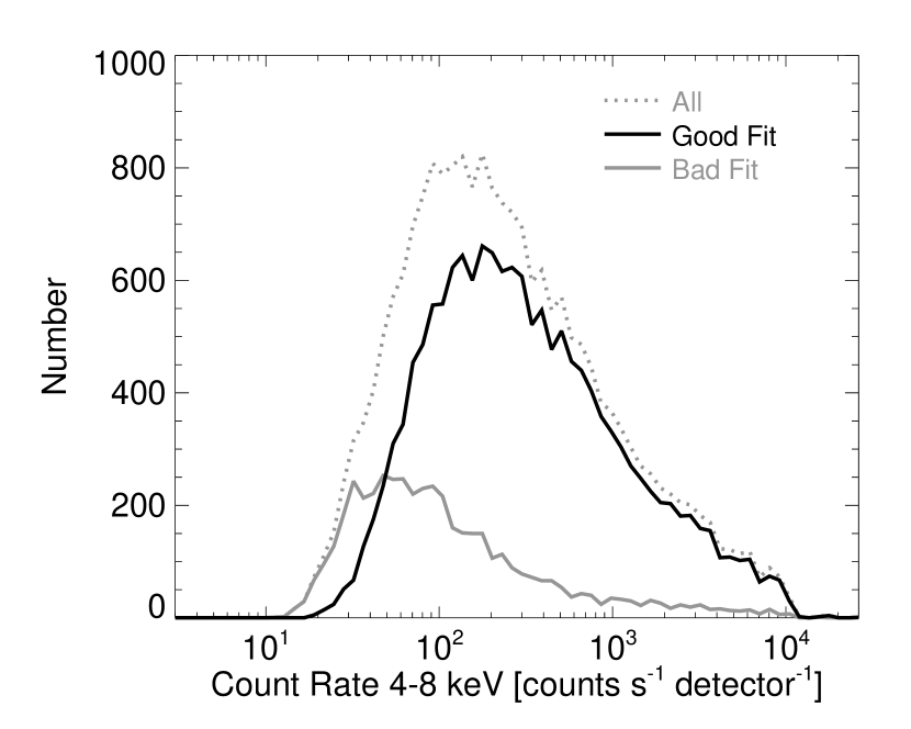
Figure 3.— Histogram of the count rate per detector in 4-8 keV, the different lines indicating all microflares (light grey dotted) and subsets with a good (solid black) and bad (solid grey) model fits to the visibilities.

The model fit for each of the microflares not only provides the spatial information but also a measure of the “quality” of the fit, based upon whether the fit converged, whether the fit parameters reach the limit of their range and the size of the errors relative to the parameter. Such an objective measure of the fit quality is vitally important for an automated analysis project as it is impractical to visually inspect over 25,000 images. After processing all microflares we have 18,656 microflares to which the model achieved a satisfactory fit and were resolved, i.e. returning spatial sizes larger than the instrumental resolution, 2.3”. The majority of events producing poor fits were those that had the fewest counts. This can be seen in Figure 3 where the histogram of the 4-8 keV count rate per detector of all the microflares is shown, as well as for the subsets of events producing good and bad fits. There are some microflares with large count rates but poor fits. This is likely due to an instrumental issue, such as to an absence of spacecraft roll information.

The histograms of the loop FWHM arc length $l$ and width $w$ (at loop mid-point) for the events with good VFFs are shown in Figure 4. We find that the median FWHM loop arc length is $31.6"$ (23 Mm) and width is $10.5"$ (8 Mm). The lengths distribution has a sharp peak, symmetrical in log-space, away from the resolution limit. The histogram of the ratio of the loop arc length to width (middle panel of Figure 4) shows that the majority of the microflare thermal sources are elongated structures, with the median value of the arc length being 3 times the loop width. The size of these loops shows no correlation with the magnitude of the flare, either the flux in the loop or the background subtracted GOES class (Figure 5). This shows that small flares are not necessarily spatially small, which is certainly the case for the examples shown in Figures 1 and 2.

The volume of this thermal emission can be estimated by assuming that the observed 2D loop structure has a cylindrical geometry as

$$V=\pi\left(\frac{w}{2}\right)^{2}l$$ (5)

where $l$ is the FWHM loop arc length and $w$ is the width at the loop mid-point. The histogram of the loop volume for the good events is shown in the right panel in Figure 4. The median volume is about $1\times 10^{27}~{}\mathrm{cm}^{-3}$, which is a factor of $\approx$66 larger than the minimum measurable volume of $1.5\times 10^{25}~{}\mathrm{cm}^{-3}$, found by taking $w=l=2.3"$ in equation (5).

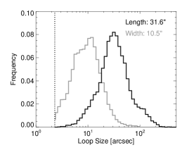
Figure 4.— (Left) Histogram of the model loop arc length and width for 18,656 RHESSI microflares. The dotted vertical line indicates the instrumental resolution limit of 2.3”. (Middle) Histogram of the ratio of 4-8 keV microflare loop length to width. (Right) Histogram of the microflare volume of the 4-8 keV loops, assuming cylindrical geometry from the 2D fitted width and length. The dotted vertical line indicates the minimum measurable model volume.

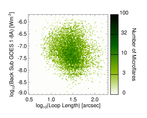
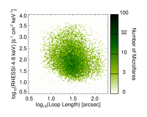
Figure 5.— Correlation plots of the model loop arc length against the background subtracted GOES 1-8 Å soft X-ray flux (top) and the RHESSI image model’s 4-8 keV flux (bottom).

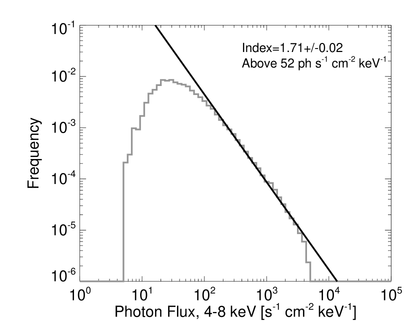
Figure 6.— Frequency distribution of the total photon flux measured from the VFF 4-8 keV loops. The power-law fit is performed using a maximum likelihood method of Parnell & Jupp (2000) and is not a graphical fit to the histogram shown.

We obtain other useful parameters from VFF, in particular a measure of the total 4-8 keV photon flux from the loop. Since unmodulated background does not affect the visibilities this flux measure is intrinsically background-subtracted as it is the emission from only the loop. In Figure 6 we have the differential frequency distribution of this 4-8 keV photon flux. This distribution covers a range of 5 to 5000 photons s^-1 cm^-2 keV^-1 and power-law parameters were found using a maximum likelihood method (Parnell & Jupp, 2000). This technique uses the standard statistical procedure of the maximum likelihood estimation to fit a skew-Laplace distribution to the data. This distribution consists of a broken power-law; the index above the break is the true distribution, whereas below it the power-law fits the flattening/turning-over of the distribution from under-sampling the smallest events. So from a simple calculation on the sample (in this case 4-8 keV fluxes) an objective measure is obtained of the power-law index above a break (with errors found from the 95% sample confidence) instead of subjectively choosing bin sizes before line fitting a histogram. For simplicity the resulting fit is shown overplotted to a standard histogram in Figure 6. Over two orders of magnitude the power-law index is $1.71\pm 0.02$. This is steeper than the index of $1.59$ found for hard X-rays $>25$ keV (Crosby et al., 1993) but flatter than the that found for soft X-rays, 1.7 – 2.1 (Drake, 1971; Lee et al., 1995; Feldman et al., 1997; Veronig et al., 2002). The distribution in Figure 6 deviates from a power-law at both low and high fluxes due to instrumental selection effects. The events with the smallest and largest fluxes are missing as we are unable to successfully analyze these events: the smallest are hard to observe above background and the largest have excessive counts causing high detector deadtime or are excluded from our microflare list as RHESSI’s attenuating shutters were deployed.

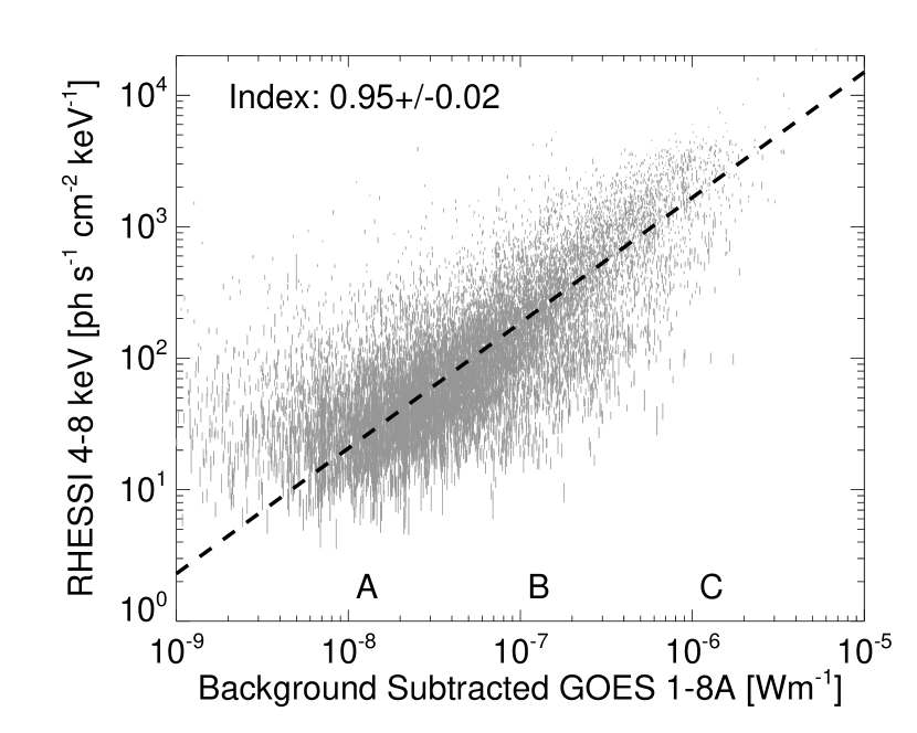
Figure 7.— Background-subtracted GOES 1-8 Å soft X-ray flux against the RHESSI image model’s 4-8 keV flux.

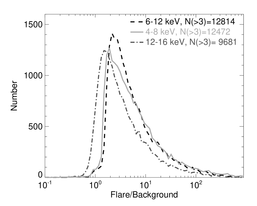
Figure 8.— Histogram of the ratio of flare signal to pre-flare background in 6-12 keV (dashed black), 4-8 keV (solid light grey) and 12-16 keV (dashed-dotted grey) at the time of peak emission in 6-12 keV.

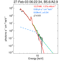
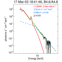
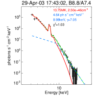
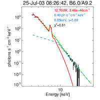
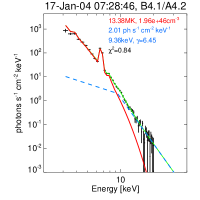
Figure 9.— Example microflare spectra. Shown are the background subtracted data (black crosses), thermal model (solid line, red in electronic edition), non-thermal model (dashed line, blue in electronic edition) and total model (solid line, green in electronic edition). The title shows the GOES class and the background-subtracted equivalent.

Another way in which we can use this RHESSI 4-8 keV thermal flux is by comparing it to the emission observed by GOES in its 1-8Å  band (Figure 7). Here we see that there is a power-law correlation, with index close to one, although there is some spread about the fitted line. This suggests that RHESSI and GOES are observing the emission from the same thermal plasma with the different temperature distribution from event to event accounting for the spread in the correlation. In comparison to RHESSI quiet Sun observations (Hannah et al., 2007), the smallest microflare flux measured here is over 2 orders of magnitude larger than the limit found from an active-region-free quiet Sun. The quiet Sun RHESSI flux also correlates with the GOES flux with a slightly steeper slope ($1.08\pm 0.13$) than the microflares shown here.

3. Spectrum Fitting

The spectrum of each microflare is determined over the same time period as the visibilities in §2, 16 seconds around the time of peak emission in 6-12 keV. These spectra are made with $1/3$ keV energy bins between 3 keV to 30 keV using detectors 1,3,4,5,8 and 9. For each microflare, a background interval before and after the event were determined automatically with the selection of these background times described in Part I of this paper (Christe et al., 2008). Only the pre-flare background is used in the subtraction from the spectrum, as it is sharply defined by the microflare’s impulsive phase. This was possible for 19,441 microflares. The histogram of the flare signal to background ratio is shown in Figure 8, for the 6-12 keV, 4-8 keV and 12-16 keV energy bands. Requiring the flare signal to be at least 3 times the pre-flare background, we find 12,814 events suitable in 6-12 keV (the energy range the events were found in) 12,472 in 4-8 keV from predominantly thermal emission and 9,681 in 12-16 keV from mostly non-thermal emission. This indicates that the thermal component for more microflares can be obtained than the non-thermal component. This does not mean that many microflares do not have a non-thermal component, just that we cannot distinguish it from the background in these cases.

These background-subtracted observed count spectra are forward-fitted with a model in photon space converted back to count space using the full RHESSI detector response matrix (Smith et al., 2002) in the OSPEX software package, an updated version of the SPEX code (Schwartz, 1996). The model has both a thermal and non-thermal component so that we can recover the respective parameters to calculate the energy in both the heated and accelerated electrons. The thermal component contains the isothermal bremsstrahlung emission (free-free and free-bound) as well as line emission from the CHIANTI database (Dere et al., 1997; Landi et al., 2006). This emission depends on the temperature $T$ and emission measure $EM=n_{\mathrm{e}}^{2}V$. The non-thermal component is assumed to be thick-target emission of a power-law distribution of electrons above a low energy cut-off $E_{\mathrm{C}}$, with the photon spectrum found through numerical integration (Holman, 2003). Although this numerical integration provides an accurate representation of the non-thermal emission it is too slow to compute in this fitting procedure, requiring multiple iterations per microflare, with tens of thousands of microflares to fit. Instead the non-thermal component is fitted with a broken power-law, which has an index of $-\gamma$ above the break energy of $\epsilon_{\mathrm{B}}$ and a fixed index of $-1.5$ below the break. An example of this approximation to the numerical integration is shown in the left panel of Figure 20 and the relationship between these two models is detailed further in §4.2, as it is important for calculating the power in the non-thermal electrons via equation (4).

The fit to each microflare spectrum is conducted using the following strategy. First the thermal parameters are varied to fit the spectrum over 4-8 keV, where the thermal emission normally dominates. Then the fit is repeated but the non-thermal parameters are allowed to vary, while keeping the previously found thermal parameters fixed, to fit the spectrum from 10 keV up to either 30 keV or to where the background dominates over the flare signal. The fit is repeated a final time allowing all the fit parameters to vary to fit the spectrum from 3 keV up to either 30 keV or to where the background dominates over the flare signal. Examples of typical microflare spectra and the fits are shown in Figure 9. The microflares here illustrate similar characteristics as seen in previous RHESSI microflare studies, for example Krucker et al. (2002). At low energies ($\leq 10$ keV) the thermal component dominates with the expected spectral lines, Fe K-shell feature (about 6.7 keV) and the Fe/Ni lines (about 8 keV), for this temperature range (Phillips, 2004). At higher energies ($\geq 10$ keV) there is a power-law component that dominates over the thermal model which is normally assumed to be the non-thermal emission. Although this could be an additional hotter thermal component several other arguments imply non-thermality: the presence of the Neupert effect (Benz & Grigis, 2002) in some cases, imaged hard X-ray footpoints (Krucker et al., 2002), and complementary radio and microwave observations (Liu et al., 2004; Qiu et al., 2004; Kundu et al., 2005, 2006).

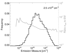
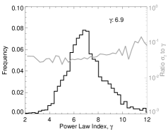
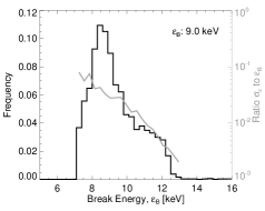
Figure 10.— (Top) Histogram of the microflare temperature (left) and emission measure (right) from the spectral fits of 9,161 RHESSI microflares. (Bottom) Histogram of the photon power-law index $\gamma$ (left) and break energy $\epsilon_{\mathrm{B}}$ (right) for 4,236 RHESSI microflares. The grey lines in each panel refer to the righthand axis and show the average ratio of the error in the fit to the fitted parameter, as a function of the parameter.

As with the imaging, the spectral fitting returns parameters that objectively measure the quality of the fit, such as the fit $\chi^{2}$ or whether the fit parameters have large errors or reach the limit of their chosen fitting range. We obtain 9,161 events for which we trust the fit to the thermal component of the spectrum and the forward fit model loop. This is out of a possible 9,693 microflares with good background subtraction, flare signal-to-background over 4-8 keV and a successful model fit. For the thermal and non-thermal fit as well as the VFF model loop fit to the visibilities we obtain 4,236 trustworthy events. This is out of a possible 8,046 microflares with good background subtraction, flare signal-to-background over 10-12 keV and successful model fit. The histograms of these fitted parameters are shown in Figure 10 and discussed in §3.1 and §3.2.

3.1. Thermal Parameters

The histograms of the fitted temperature and emission measure for the events with good background subtractions and thermal fits, 9,161 microflares, are shown in the top row of Figure 10. This is about a third of the total sample but shows nearly all of the events with good background subtraction, flare signal-to-background and visibility forward fits (9,693 microflares). The majority of the temperatures found lie within a tight range of about 10 to 15 MK, with the median temperature of around 13MK. The emission measures vary considerably more than the temperatures, having a range covering over two orders of magnitude between $10^{45}$ to $10^{47}$ cm^-3. The median emission measure is $3\times 10^{46}$ cm^-3. Also shown in Figure 10 are the average ratio of the error in the fit to the fitted parameter. For the temperatures this statistical error in the fit is $<1\%$ and is approximately constant for the temperatures found. The error in the emission measure is $\approx 10\%$ at $10^{45}$ cm^-3 but drops to $\approx 1\%$ at $10^{47}$ cm^-3. The larger relative error in the events with smallest emission measure is due to the emission measure being directly proportional to the thermal emission model, and so are events with small noisy spectrum. The range of these parameters is discussed further in §3.3. With these emission measures and the volumes of the emitting plasma (see §2) an estimate of the electron density can be made. The histogram of these densities is shown in Figure 11 and range from $6\times 10^{8}$ to $6\times 10^{10}$ cm^-3 with median value of $6\times 10^{9}$ cm^-3. This is larger than typical coronal conditions but reasonable for a flaring loop (Phillips et al., 1996; Gallagher et al., 1999).

Figure 11.— Histograms of the density of the 4-8 keV loops, found from the emission measure and thermal volume for 9,161 RHESSI microflares.

Figure 12.— Histogram of the ratio of the 4-8  keV flux found from the fitted spectrum model and the image model loop.

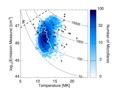
Figure 13.— Microflare temperature against emission measure. The correlation plot is the microflares in this study with black crosses representing the results of a previous RHESSI study (Battaglia et al., 2005). The dashed straight line represents the correlation found by Feldman et al. (1996b) from GOES and Yohkoh/BCS. The numbered curved lines are of constant count rate per detector in 4-8 keV for the thermal model, as a function of temperature and emission measure. The white contour show the events that have a GOES temperature $<10$ MK in Figure 14.

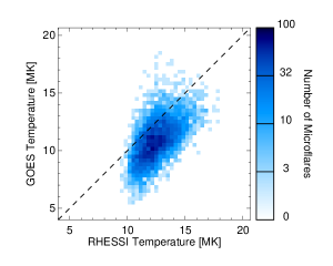
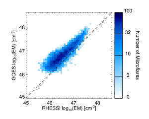
Figure 14.— Correlation plots of temperature (top) and emission measure (bottom) from RHESSI and GOES for the same peak time in RHESSI 6-12 keV for 6,740 microflares. The dashed lines indicate a one-to-one correlation.

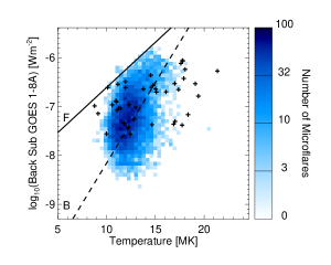
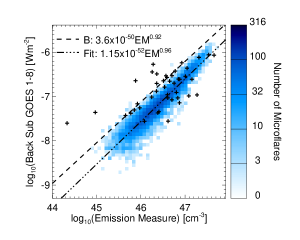
Figure 15.— Microflare temperature (top) and emission measure (bottom) against the background subtracted GOES 1-8Å flux. The correlation plots are the microflares in this study, with the dot-dashed line (bottom panel) the fit to this data. The black crosses and dashed line were found from a previous RHESSI study (Battaglia et al., 2005). The solid line (top panel) represents the correlation found by Feldman et al. (1996b).

With these fitted thermal components we can estimate the 4-8 keV flux from these spectrum fits and compare it to the flux derived from the imaging in §2. This provides a consistency check to verify that these two vastly different analysis techniques recover similar fluxes. The histogram of the ratio of the flux found from the spectrum model to the image value is shown in Figure 12. The median of these is $1.0$ with some spread about this value. This is expected as different detectors were used for imaging and spectral analysis (additional use of detector 5 in imaging) and the imaging calculation uses only the diagonal elements of RHESSI’s detector response matrix, (Smith et al., 2002), whereas the spectrum fitting uses the full response matrix.

3.2. Non-thermal Parameters

Histograms of the index $\gamma$ and break energy $\epsilon_{\mathrm{B}}$ of the non-thermal broken power-law are shown in the bottom row of Figure 10. The power-law index $\gamma$ has values mostly ranging over 4 to 10 with the median about 7. This is considerably steeper than large flares observed by RHESSI, as discussed in previous RHESSI microflare work (Krucker et al., 2002; Benz & Grigis, 2002). The break energy $\epsilon_{\mathrm{B}}$ ranges over 7 keV to 12 keV with the median being about 9 keV, which is smaller than is found for larger flares (Saint-Hilaire & Benz, 2005). In larger flares, the lower energy non-thermal emission would be masked by the thermal emission to tens of keV. The steep power laws starting at low energies leads to a strong selection effect. This is because such steep power-laws, extending down to energies where there are spectral lines (Phillips, 2004), are difficult to distinguish from a thermal component. A conservative approach has been taken here to remove any events where there is an ambiguity between the thermal and non-thermal components, so we discount any events any events with $\epsilon_{\mathrm{B}}\leq 7$ keV. The result is that we have only 4,236 microflares, about a fifth of the total sample.

Also shown in Figure 10 are the average ratios of the error in the fit to the fitted parameter. For the power-law index $\gamma$ this statistical error in the fit is $\approx 4\%$ for $\gamma<8$ and increases to $\approx 10\%$ for $\gamma>8$. This increase in the error shows the greater uncertainty in trying to fit steep spectrum. The error in the break energy is $\approx 10\%$ at about $\epsilon_{\mathrm{B}}=7$ keV and decreases to $>1\%$ by $\epsilon_{\mathrm{B}}=12$ keV. The large errors at low break energies shows the greater uncertainty in trying to separate the thermal and non-thermal components below 10 keV. These non-thermal parameters are discussed further in §4.2.

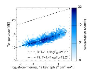
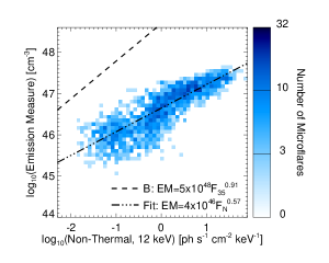
Figure 16.— RHESSI non-thermal photon flux at 12 keV, from the fitted broken power-law, against fitted temperature (top) and emission measure (bottom). The correlation plots are the microflares in this study, the fit to this data is the dot-dashed line. The dashed line is from a previous RHESSI study using the non-thermal flux at 35 keV (Battaglia et al., 2005).

3.3. Correlation Between Parameters

Figure 13 plots the temperature against emission measure for the RHESSI microflares. There is no clear correlation between these parameters. Also shown are numbered contours indicating constant count rate per detector over 4-8 keV for the thermal model as a function of temperature and emission measure. All of the microflares lie between the 10 and 10⁴ counts s^-1 contours, consistent with the non-background subtracted count rates for good fits shown in Figure 3. Although any temperature and emission measure between these contours could be expected, the temperatures lie in a tight range, mostly between 10 MK and 15 MK, with almost all possible emission measures, from $10^{45}~{}\mathrm{cm}^{-3}$ to $10^{47}~{}\mathrm{cm}^{-3}$, for this temperature range found. The model of the thermal emission is directly proportional to $EM$ and increases with larger $T$, though not directly, with the continuum rising and flattening and the line features becoming more prominent (Tandberg-Hanssen & Emslie, 1988). This results in the errors in the temperature and emission measure being anti-correlated. The thermal model also includes spectral features and they provide additional emission, particularly from the Fe K-shell over 4-8  keV, for temperatures above $8$ MK (Phillips, 2004). The fact that only temperatures above $8$ MK have been found is more suggestive of a selection effect primarily affecting the temperatures and not a physically significant discovery of microflares with a lack of low temperatures and high emission measures. This selection effect is consistent with RHESSI’s sensitivity being temperature-dependent. The combination of this greater sensitivity to hotter plasma and the differential emission measure DEM decreasing as the temperature increases could explain the tight range of temperatures found with the peak of this sensitivity for RHESSI shutter-out mode occurring in this temperature range. Note that this selection effect essentially does not reject any event detectable by GOES.

Microflares analyzed in a previous RHESSI spectral study of flares of all scales, 42 microflares out of a sample of 85 flares, (Battaglia et al., 2005) are shown as the crosses in Figure 13 and also showed no correlation. These events specially chosen to cover a wide range of RHESSI flare magnitudes were analyzed during the peak in 12-25 keV. This is earlier in the flare phase than for our survey. Thus they have correspondingly higher temperatures and lower emission measures. Another recent study of 18 microflares from a single active region (Stoiser et al., 2007) found similar results to the Battaglia et al. (2005) study.

The dashed line in Figure 13 is the correlation found using soft X-ray observations with GOES and Yohkoh/BCS (Feldman et al., 1996b), for all size of flares from A through to X class, not just microflares. This correlation has a order of magnitude spread in emission measure and only becomes apparent when a large range of flare magnitudes are included; for only small A-class events the correlation was in the opposite direction (Feldman et al., 1996a) with the emission measure decreasing with increasing temperature. In comparison the RHESSI data, which is observed at higher energies than Feldman et al. (1996b), show higher temperature and/or lower emission measures. This is consistent with the DEM peaking at temperatures lower than those observed with RHESSI and closer to those lower temperatures observed by GOES and Yohkoh/BCS. This was found to be case for the DEM of a large flare observed in soft X-rays with GOES and Yohkoh/SXT and in hard X-rays with Yohkoh/HXT (Aschwanden & Alexander, 2001). For RHESSI emission measures above $8\times 10^{46}~{}\mathrm{cm}^{-3}$ there is the hint of a similar correlation with temperature but it is obscured by the temperature selection effect at lower emission measures. Further studies of solar flare temperature and emission measure suggested that the emission measure of EUV nanoflares approximately scales as $T^{5}$ (Aschwanden et al., 2000), but using various studies over larger scales suggested the emission measure may scale as $T^{4}$ (Aschwanden, 2007). These scalings are only approximate as there is large scatter about the correlation line. Looking over larger ranges with different instruments helps to reduce the overall influence of the selection effects but there is still ambiguity as to how these parameters scale.

To gain a better understanding of the RHESSI temperature and emission measure, we have also calculated the GOES temperatures and emission measures for each of these microflares. This was done using the same pre-flare time for background and peak time of emission in 6-12 keV as was used in the RHESSI analysis. This was possible for 6,740 microflares, removing those events for which a GOES temperature and emission measure were not reliably calculable. The resulting correlation plots are shown in Figure 14. The bottom right hand of this correlation plot (the lowest GOES temperature for each RHESSI temperatures) does seem to be directly proportional, except the RHESSI temperatures are about 5 MK higher. The rest of the plot is again dominated by the selection effect in the RHESSI temperatures. The events with GOES temperature $<10$ MK have been highlighted by the white contour in Figure 13. If the assumption is that the RHESSI temperate estimate is too high in these events, and the emission measures is consequently too small, then this set of highlighted events should be moved upwards and to the left in Figure 13. This shift produces a clearer hint of the previously found correlation between temperature and emission measure.

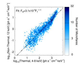
Figure 17.— RHESSI non-thermal flux at 12 keV, from the fitted broken power law, against the the thermal flux over 4-8 keV, from the thermal model. The dot-dashed line is the fitted correlation line.

The emission measures in Figure 14 do not show any such temperature selection effect and are nearly directly proportional, with the GOES emission about twice that observed in RHESSI. Again this will be due to RHESSI observing in a temperature range which is higher than the peak temperature in the DEM. The proportionality between the RHESSI and GOES emission measures on face value suggests a similarly steep DEM in all the microflares but this might be arising from the relative instrumental sensitives. It is important to remove these instrumental effects to recover the underlying DEM but this is a complicated process and has only been successful for individual large flares, (c.f. Aschwanden & Alexander, 2001).

Other studies (Feldman et al., 1996b; Battaglia et al., 2005) have also investigated how the temperature and emission measure relate to the GOES flux of the events. The RHESSI microflare temperature and emission measure plotted against each event’s corresponding background-subtracted GOES 1-8Å is shown in Figure 15. Again there is a hint of a correlation between the RHESSI temperature and GOES flux for the events above B-class ($10^{-7}~{}\mathrm{Wm}^{-1}$), but it is obscured in smaller events again due to the temperature selection effect. The previous study of RHESSI flares (Battaglia et al., 2005) found a correlation when using large flares in addition to microflares. This correlation and the microflares in their sample are shown in Figure 15, by the dashed line and crosses, and is steeper than found using GOES and Yohkoh/BCS (Feldman et al., 1996b). The hint of a correlation in our microflare study scales in a manner closer to Feldman et al. (1996b) than Battaglia et al. (2005), although the temperatures found are consistently higher.

There is a clear correlation between the emission measure and GOES flux, which can be fitted as $F_{\mathrm{G}}=1.15\times 10^{-52}EM^{0.96}$, with $F_{\mathrm{G}}$ in Wm^-2 and $EM$ in cm^-3. A similar result was also found in the Battaglia et al. (2005) study, fitted over a large flare to microflare range finding $F_{\mathrm{G}}=3.6\times 10^{-50}EM^{0.92}$. The consistently lower emission measures in this study are again due to this analysis occurring earlier in the microflare than in our study.

We can also investigate how the non-thermal emission relates to the thermal parameters, which is shown in Figure 16. Here the non-thermal flux $F_{\mathrm{N}}$, in units of photon flux at Earth $\mathrm{s}^{-1}\mathrm{cm}^{-2}\mathrm{keV}^{-1}$, is taken from the fitted broken power-law parameters at 12 keV. This energy is used as it is above the break energy $\epsilon_{\mathrm{B}}$ in all events but is still at an energy for which we observe non-thermal emission. Both the temperature and emission measure scale with the non-thermal emission. The correlation with the temperature is fitted as $T=1.41\log{F_{\mathrm{N}}}+13.2$, with $T$ in MK. A similar correlation was found in the Battaglia et al. (2005) study using the flux at 35 keV for the non-thermal flux, since larger flares were also analyzed, finding $T=1.46\log{F_{\mathrm{35}}}+21.57$. We find that the scaling of the emission measure is flatter, $EM=4\times 10^{46}F_{\mathrm{N}}^{0.57}$, compared to the previous study $EM=5\times 10^{48}F_{\mathrm{35}}^{0.91}$ (Battaglia et al., 2005), again $EM$ in units of cm^-3.

In Figure 17 this non-thermal photon flux at 12 keV $F_{\mathrm{N}}$ is plotted against the model thermal flux over 4-8 keV, $F_{\mathrm{T}}$. The thermal and non-thermal emission correlate, with the fit being $F_{\mathrm{N}}=3.4\times 10^{-3}F_{\mathrm{T}}^{1.09}$, but with a greater scatter in the smaller events. At higher fluxes the correlation steepens, suggesting that there might a greater proportion of non-thermal emission relative to thermal emission in larger flares. However, this may just be an instrumental effect, arising from detector pileup and livetime issues in these larger events prior to the shutters deploying.

4. Energy Distributions

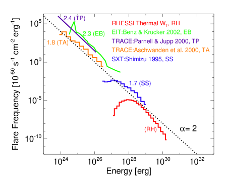
Figure 18.— Frequency distribution of the thermal energy, of 9,161 RHESSI microflares (RH) in context of thermal energy distributions of nanoflares (TA, TP and EB) and active region transient brightenings (SS). The dotted line indicated a power-law index of $\alpha=2$.

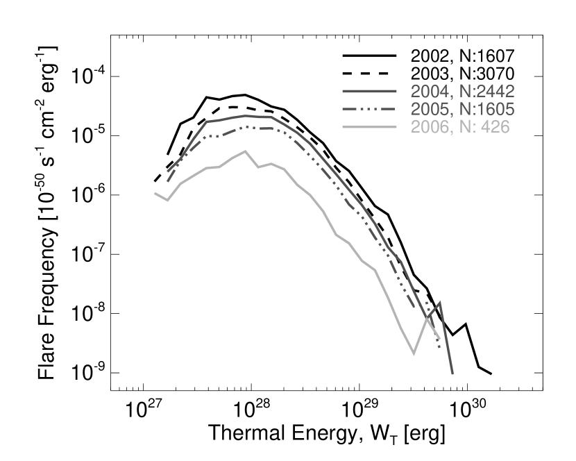
Figure 19.— Frequency distribution of the microflare thermal energy, each line indicating a different year. The number quoted next to the year is the number of events from each year used in the distribution.

4.1. Thermal Energy Frequency Distributions

Using the volumes found in §2 and temperature and emission measure found in §3 the thermal energy $W_{\mathrm{T}}$, over the time of peak emission in 6-12 keV, can be calculated via equation (3). The energies range from $10^{26}$ erg to $10^{30}$ erg with the median being about $10^{28}$ erg. The frequency distribution (number of events per energy bin range, area of solar disk and duration of observation period) of this energy for 9,161 microflares is shown in Figure 18. The resulting RHESSI thermal energy distribution is not a clear power-law; it has a turn-over at low energies and steepens at higher energies. These features are instrumental effects due to missing the smallest events, with insufficient counts to either find the events or successfully analyze them, and the largest events, due to detector livetime issues before the attenuating shutters come in. Considerably more small events are missing than large, since the discrepancy from a power-law is greater at lower energies than high. As this distribution deviates from a power-law it will not be fitted to obtain the power-law index $\alpha$. Instead, Figure 18, shows an $\alpha=2$ line, indicating the parts of the RHESSI thermal distribution can be steeper and flatter, or larger and smaller, than $\alpha=2$.

Compared to the previous distributions found for EUV nanoflares (Krucker & Benz, 1998; Aschwanden et al., 2000; Parnell & Jupp, 2000; Benz & Krucker, 2002) and soft X-ray active-region transient brightenings (Shimizu, 1995), the RHESSI energy distribution appears as an extension to these at higher energies. This is both remarkable and deceptive since these distributions were found for very different types of events, using various instruments and for different periods during the solar cycle. For instance the SXT energies (Shimizu, 1995) are from 291 brightenings in one active region over 5 days in August 1992, whereas the EIT (Krucker & Benz, 1998; Benz & Krucker, 2002) and TRACE EUV quiet sun observation (Aschwanden et al., 2000; Parnell & Jupp, 2000) were found over about an hour each on 12 July 1996, 17 February 1998 and 16 June 1998 respectively. So there are two key issues that have to be taken into account when looking at the energy distributions in Figure 18. First, various instruments were used, so different components of the thermal energy will be observed and with distinctive instrumental selection effects will influence each distribution. This makes it difficult to determine whether these are similar events or completely distinctive physical processes. Second, the distributions cover different phases of the solar cycle. The previous studies show a snapshot of the energy distribution of different small energy release features in the solar corona whereas the RHESSI microflare energy distribution represents 5 years of observations of the declining phase of the solar cycle. The difficulty here lies in determining whether these snapshot surveys demonstrate typical or unusual behavior. Using the RHESSI thermal energies we can investigate how the energy distribution changes with time by plotting the distributions for each year separately, as shown in Figure 19. These distributions have similar shapes except that the normalization decreases by over an order of magnitude between 2002 and 2006. So the non-RHESSI distributions in Figure 18 could be shifted vertically by a considerable amount if they were found during a different part of the solar cycle. This invariance in the shape of the distribution during the solar cycle has been found previously in both soft (Feldman et al., 1997; Veronig et al., 2002) and hard (Crosby et al., 1993; Lu et al., 1993) X-rays, and also illustrates that the selection effects on the RHESSI data do not vary with time.

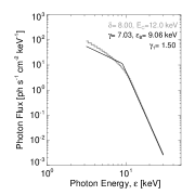
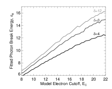
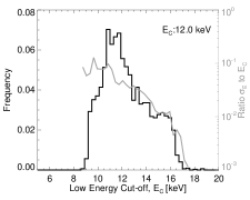
Figure 20.— (Left) Broken power-law fit to photon spectrum from a thick target model of a power-law electron distribution, using the code of Holman (2003). (Middle) Fitted break energy $\epsilon_{\mathrm{B}}$ of photon broken power-law against low energy cut-off of electron distribution, the different lines indicate the different indices $\delta$ of the electron distributions. (Right) Histogram of $E_{\mathrm{C}}$ for the 4,236 microflares shown in Figure 10. The grey line refers to the righthand axis and shows the average ratio of the error to $E_{\mathrm{C}}$ as a function of $E_{\mathrm{C}}$.

4.2. Non-Thermal Power Frequency Distributions

To calculate the power in accelerated electrons from the information about the power-law in the photon spectrum, we use $\gamma$ and $I_{\mathrm{0}}$ (the power-law index and normalization), found in §3, in equation (4). However there is ambiguity as to the low-energy cut-off $E_{\mathrm{C}}$ because the observed photon spectrum depends only weakly on it. In addition the RHESSI microflare spectrum covers both the thermal and non-thermal energy ranges and so there is inherent ambiguity. Previous studies used their X-ray threshold for $E_{\mathrm{C}}$ resulting in large uncertainties in the energy estimates (Crosby et al., 1993; Lin et al., 2001). As RHESSI makes spectral measurements down to the thermal component we can provide a better estimate of the non-thermal energy content. In Part I of these papers a fixed $E_{\mathrm{C}}$ was used to provide a rough estimate of the non-thermal power at peak time (Christe et al., 2008). The full spectrum fitting in §3 provides a better estimate of the parameters required to calculate the non-thermal power via equation (4). However, despite this improvement we only have an estimate of where the photon spectrum begins to flatten $(\epsilon_{\mathrm{B}})$ and not the actual cut-off in the electron distribution $E_{\mathrm{C}}$.

To obtain an estimate of $E_{\mathrm{C}}$ we have therefore investigated how the fitted broken power-law model relates to the expected photon spectrum from the electron distribution using the numerical integration code of Holman (2003). An example of this is shown in the left panel of Figure 20, where the photon spectrum for an electron distribution with $\delta=8$ and $E_{\mathrm{C}}$ was calculated and then fitted with a broken power-law in the same manner as was used for the microflare spectrum. This broken power-law has $\gamma=7.03$, expected as $\delta\equiv\gamma+1$ (Brown, 1971), above a break of $\epsilon_{\mathrm{B}}=6.06$ keV. Repeating this process for various values of the electron distribution parameters $\delta$ and $E_{\mathrm{C}}$, shows how the resulting fitted $\epsilon_{\mathrm{B}}$ scales with these parameters. This is shown in the middle panel in Figure 20, where $\epsilon_{\mathrm{B}}$ is given against $E_{\mathrm{C}}$ for three different values of $\delta$. For a single value of $\delta$, $E_{\mathrm{C}}$ approximately scales linearly with $\epsilon_{\mathrm{B}}$ and this scaling steepens with increasing $\delta$. So we can approximate this relationship to first order by linearly fitting the relationship between $\epsilon_{\mathrm{B}}$ and $E_{\mathrm{C}}$ for various $\delta$ and then linearly fitting how the parameters of the first fit vary with $\delta$. This empirical relationship between the observed parameters of the photon power-law $\gamma,\epsilon_{\mathrm{B}}$ and the low energy cut-off of the electron distribution $E_{\mathrm{C}}$ can be found:

$$E_{\mathrm{C}}\approx 0.15\gamma+(1.86-0.04\gamma)\epsilon_{\mathrm{B}}-3.39.$$ (6)

Using equation (6) the values of $\gamma$ and $\epsilon_{\mathrm{B}}$ for the 4,236 microflares with trustworthy non-thermal spectral fits result in a histogram of $E_{\mathrm{C}}$ for these events, shown in the right panel in Figure 20. The low energy cut-offs range from 9 to 16 keV with the median being about 12 keV, with generally $\epsilon_{\mathrm{B}}\approx 0.75E_{\mathrm{C}}$. The uncertainty in $E_{\mathrm{C}}$ can be seen in the average ratio of the error (found from the fit errors in $\gamma$ and $\epsilon_{\mathrm{B}}$) to $E_{\mathrm{C}}$ also shown in the right panel of Figure 20. For $E_{\mathrm{C}}<12$ keV, where the major of the event lie, the uncertainty is about $10\%$ and drops to about $1\%$ for the few events with larger $E_{\mathrm{C}}$.

These values of $E_{\mathrm{C}}$ can then be used in equation (4) to calculate the power in non-thermal electrons above $E_{\mathrm{C}}$, $P(\geq E_{\mathrm{C}})$, the frequency distribution of which is shown in the left panel in Figure 21. Here the power ranges over $10^{25}$ to $10^{28}$ erg s^-1 with the median being about $10^{26}$ erg s^-1. Also shown is the ratio of the error to the power, as a function of the power. The few microflares which show a power of around $10^{28}$ erg s^-1 have the smallest errors with uncertainties about $10\%$. These powers seem relatively high for small flares, as the RHESSI power estimates in large flares are $10^{27}$ to $10^{30}$ erg s^-1 (Holman, 2003; Emslie et al., 2004; Saint-Hilaire & Benz, 2005; Sui et al., 2005, 2007), though it should be noted that the non-thermal emission in microflares lasts for $\approx 10$ seconds whereas it can last for tens of minutes in large flares. The total non-thermal energy content in large flares is many orders of magnitude larger than in microflares. The majority of the microflares shown in Figure 21 show non-thermal powers considerably smaller than this level, although with increasing uncertainty. The median power of $10^{26}$ erg s^-1 has about a $50\%$ error and the smallest events at $10^{25}$ erg s^-1 have almost $100\%$ error. It is this large uncertainty in the power that results in this distribution deviating from a power-law. Although the selection effects and biases will affect this non-thermal distribution as seen in the thermal distribution, these effects are hidden by the large uncertainties. Since it deviates from a power-law, it has not been fitted using this model.

To allow comparison to the power distribution in electrons above 25 keV $P(\geq 25)$ for 2,878 large flares found over 1980 to 1982 using SMM/HXRBS (Crosby et al., 1993) the same power is estimated in the RHESSI microflares, shown in the right panel in Figure 21. These powers using $E_{\mathrm{C}}=25$ keV for the RHESSI microflare ranges over $10^{22}$ to $10^{27}$ erg s^-1 with the median power being about $10^{24}$ erg s^-1. On this basis the RHESSI microflares cover events down to two orders of magnitude smaller than those in the SMM/HXRBS study. Again the error is smallest in the largest power estimates. This $P(\geq 25)$ RHESSI distribution deviates less from a power-law than the $P(\geq E_{\mathrm{C}})$ distribution. This is because there is less uncertainty in the power estimate in the larger events as the fixed $E_{\mathrm{C}}=25$ keV has no associated error.

5. Discussion & Conclusions

We have analyzed 25,705 microflares, successfully recovering trustworthy spatial information about the thermal emission for 18,656 of them, as well as the thermal spectral fit in 9,161 and the thermal and non-thermal fit in 4,236. The median values and ranges of each of the microflare parameters are summarized in Table 1. As found in Part I (Christe et al., 2008) the microflares occur only in active regions and this immediately suggests that these events are ill-suited to heat the overall corona. It also helps to show that the X-ray emission outside active regions, especially during periods of quiet Sun, is considerably smaller than the smallest active-region flares observed with RHESSI. This is confirmed by the RHESSI quiet Sun study (Hannah et al., 2007) which found a limit on the flux over two orders of magnitude smaller than that of the smallest microflares found here.

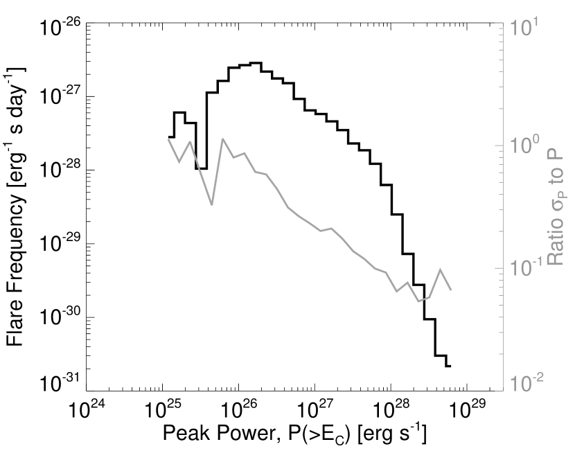
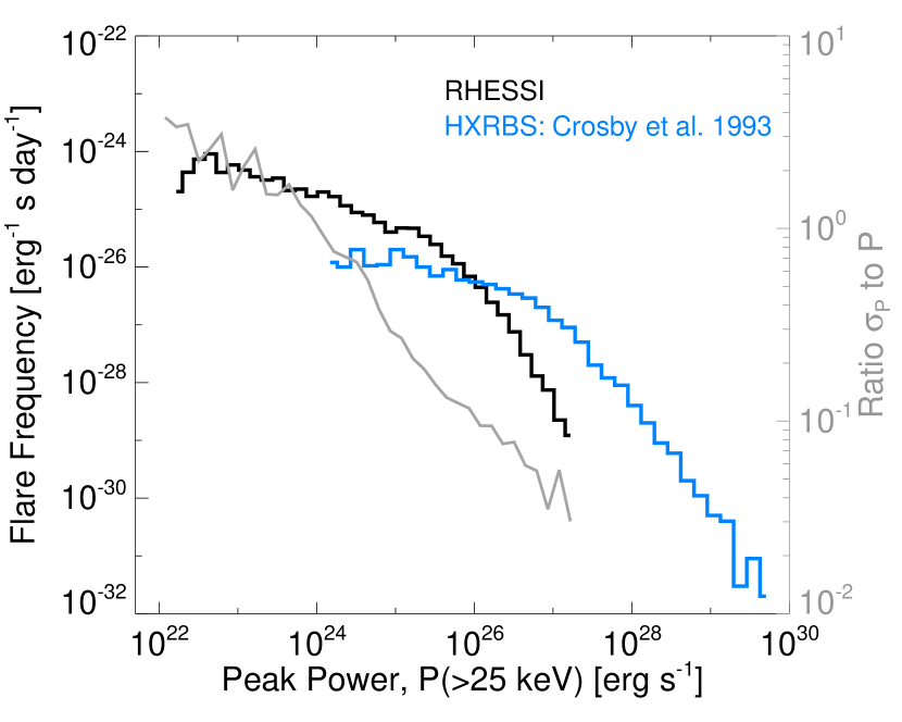
Figure 21.— Frequency distribution of the non-thermal power of 4,236 RHESSI microflares for $P(>E_{\mathrm{C}})$ (left) and $P(>25\mathrm{keV})$, in comparison to the distribution found by (Crosby et al., 1993) for large flares (right). The grey lines refers to the righthand axes and show the average ratio of the error in the power to the power, as a function of the power.

Forwarding-fitting the visibilities of RHESSI data is a fast and efficient way to recover the spatial information (Hurford et al., 2005). We find that the thermal emission (4-8 keV) of the microflares shows predominantly loop-like structures that have a median width of 11^′′ and 32^′′ length. Those events where no spatial information was recoverable were predominantly those with the fewest counts, although some larger events produce poor spatial information as there were other instrumental issues. These spatial scales do not correlate with the magnitude of the microflare, the 4-8 keV flux from the loop nor the GOES class, and so small flares are not necessarily spatially small. This may be due to the prevalence of a typical loop scale size associated with active regions, and it is independent of the amount of energy the flare has deposited into heating the material that evaporates to fill these loops. In the largest flares this energy might be deposited over a larger area, evaporating material into more loops, hence the larger structures and arcades that are observed. The widths of these loops may not be as well resolved as the lengths, with the observed single RHESSI loop possibly being several narrow and long loops beside each other, as observed in microflare with RHESSI and Hinode/XRT (Hannah et al., 2008). The volume of these loops can be estimated, the median value being $1\times 10^{27}~{}\mathrm{cm}^{3}$. This volume estimate assumes a cylindrical geometry and filling factor of unity, meaning that our volumes, and hence thermal energies, are upper limits, as this filling factor can be $<1$ (Cargill & Klimchuk, 1997; Takahashi & Watanabe, 2000).

We find that microflares are hot, with a median temperature of 13 MK. In these microflares the median emission measure is $3\times 10^{46}~{}\mathrm{cm}^{-3}$, which combined with the volume allows a density of $6\times 10^{9}~{}\mathrm{cm}^{-3}$ to be calculated. As the volume may be an overestimate, this means that the density might be underestimated. The presence of the spectral feature due to the Fe K-shell transitions proves that there really is hot plasma present with $\mathrm{T}>8$ MK (Phillips, 2004). Correlations between the temperature and other parameters are difficult to extract from our sample due to the temperature selection effect, resulting in only a relative narrow range of temperatures being sampled. Studying larger flares would aid by extending the range of flare temperatures, but this would be complicated by systematic effects related to RHESSI’s attenuating shutters. An alternative would be to investigate this selection effect by comparing model spectra for known temperatures and emission measures with those found by fitting this spectrum once noise and the instrumental response have been included. This has already been attempted for the TRACE nanoflares study (Aschwanden & Parnell, 2002), and it revealed a difference between the observed parameters and the “intrinsic” ones. Another way of investigating the instrumental response and biases is in comparison to results from other instruments. We have found that the GOES emission measures are typically a factor of 2 larger than those found with RHESSI. This maybe due to the underlying DEM in microflares scaling similarly but might also be due to the instrument’s relative sensitivity. This could be further studied by forward-fit modeling of the instrumental responses to recover the underlying DEM in each event (Aschwanden & Alexander, 2001), instead of assuming a constant emission measure.

The thermal energies for the peak time in these microflares were found to range from $10^{26}$ erg to $10^{30}$ erg with the median energy being $10^{28}$ erg. The thermal energy distribution deviates from a power-law at low and high energies but this can be explained by selection effects and does not suggest that the underlying true distribution is not power-law. The smallest events are missing as they do not have enough counts to be found either above solar or instrumental background, successfully imaged or spectrally analyzed. The larger events are missing from the distribution due to RHESSI’s attenuating shutters, so either they are exclude from our selection or have poor detector livetime. Although it is possible to extend this energy distribution to higher energies by analyzing all large flares observed with RHESSI, there will still be a strong instrumental effect at the shutter transition due to detector livetime effects. The statistical errors in the fitted parameters will affect the thermal energy estimates but these have a relatively small effect compared to the selection effects. The greatest uncertainty is the systematic error that arises from the filling factor used to estimate the thermal volume: taking an extreme filling factor of $f\approx 10^{-4}$ (Cargill & Klimchuk, 1997) would have the effect of reducing the energies by a factor of 100. Therefore the thermal energies quoted here about the time of peak emission in 6-12 keV are upper limits. The comparison of the RHESSI thermal distribution to other the thermal distributions of other transient coronal energy releases is difficult as these events are from a limited sample of events over a very short time period.

With RHESSI we are able to investigate the flattening of the non-thermal photon spectrum and can empirically estimate the low energy cut-off $E_{\mathrm{C}}$ in the electron distribution from the observed photon spectrum. However we are only able to successfully fit the non-thermal spectral component, in addition to the thermal component, in 4,236 events. The difficultly in successfully finding and fitting this non-thermal emission arises from the steep spectra that start close to the thermal spectral features about 7 keV. So, although the non-thermal component was only successfully fitted in a minority of events, it does not mean that there is a lack of accelerated electrons in the others. It does mean however that the relatively large uncertainties in the non-thermal parameters will result in large uncertainties in $E_{\mathrm{C}}$ and the non-thermal power estimates. These large uncertainties and the biases introduced by rejecting many events due to poor spectra fits can be easily seen in the histograms of the non-thermal parameters $\gamma$ and $\epsilon_{\mathrm{B}}$. We find that the microflares typically have non-thermal emission represented by a broken power-law with index $\gamma=7$, break at 9 keV. We can estimate $E_{\mathrm{C}}=12$ keV, for breaks in the photon spectrum above 7 keV.

These non-thermal parameters were used to calculate the power in accelerated electrons above $E_{\mathrm{C}}$, which range over $10^{25}$ to $10^{28}$ erg s^-1 with a median value of $10^{26}$ erg s^-1. This distribution again deviates from a power-law at low and high energies due to the uncertainties in the power estimates and the rejected events due to poor spectra fits rather than the selection effects present in the thermal distribution. The uncertainties in the few events with the largest non-thermal component are only $\sim 10\%$ and so this cannot explain the fact that in some of these small flares the rate of energy release is comparable to larger flares, $10^{27}$ to $10^{30}$ erg s^-1 (Holman, 2003; Emslie et al., 2004; Saint-Hilaire & Benz, 2005; Sui et al., 2005, 2007). However the non-thermal emission in microflares lasts for only $\approx 10$s seconds whereas it can last for tens of minutes in large flares. The non-thermal energy content in large flares is thus many orders of magnitude larger than in microflares. To make a direct comparison of these RHESSI microflare results to the peak non-thermal power distribution found for large flares by Crosby et al. (1993), the same instrumental $E_{\mathrm{C}}=25$ keV has to be used. On this basis the RHESSI microflare peak powers extend to two orders of magnitude smaller than the (Crosby et al., 1993) study. The true non-thermal power in the Crosby et al. (1993) flares cannot be determined as the spectrum was not observed to sufficiently low energies and so that study could have easily under-estimated the non-thermal energy content. We conclude that the instantaneous non-thermal power in a microflare can be surprisingly large.

Table 1 Median and range of RHESSI microflare parameters.

Microflare Parameter		Median Value	Range (5% to 95%)
Duration	$D$	5.4 mins	2.2-15 mins
Temperature	$T$	$12.6$ MK	$10.7-15.5$ MK
Emission Measure	$EM$	$3\times 10^{46}$ cm-3	$4\times 10^{45}-2\times 10^{47}$ cm-3
Thermal Loop Width	$w$	8 Mm ($11^{\prime\prime}$)	3-20 Mm ($4-28^{\prime\prime}$)
Thermal Loop Length	$l$	23 Mm ($32^{\prime\prime}$)	7-77 Mm ($10-107^{\prime\prime}$)
Thermal Loop Volume	$V$	$1\times 10^{27}$ cm3	$5\times 10^{25}-2\times 10^{28}$ cm3
Density	$n_{\mathrm{e}}$	$6\times 10^{9}$ cm-3	$8\times 10^{8}-3\times 10^{10}$ cm-3
Power-law Index	$\gamma$	7	$4-10$
Break Energy	$\epsilon_{\mathrm{B}}$	9 keV	$7-12$ keV
Low Energy Cut-off	$E_{\mathrm{C}}$	12 keV	$9-16$ keV
Thermal Energy	$W_{\mathrm{T}}$	$10^{28}$ erg	$10^{26}-10^{30}$ erg
Non-thermal Power	$P_{\mathrm{N}}(\geq E_{\mathrm{C}})$	$10^{26}$ erg s-1	$10^{25}-10^{28}$ erg s-1
Non-thermal Power	$P_{\mathrm{N}}(\geq 25)$	$10^{24}$ erg s-1	$10^{22}-10^{27}$ erg s-1

One further explanation for the unexpectedly large non-thermal power in the microflares might be that the physical model used is less suited for small flares than large. The energy in the accelerated electrons was found using the standard cold thick target model (Brown, 1971). It has been suggested that for the lowest energy electrons the target is warm and not cold, and $5kT$ could be used as an approximate cut-off (Emslie, 2003). Unfortunately for the microflares, this gives an even lower cut-off at around 4–5 keV, which results in a even larger non-thermal power estimate. Nevertheless the idea of the non-thermal electron distribution smoothly transitioning into the thermal distribution seems physically more realistic than a sharp low energy cut-off and may provide a clue to the physics of the energization of the electron distribution function. Another change to the model of the hard X-ray emission would be the inclusion of free-bound emissions (Brown & Mallik, 2007), as our models currently only assume free-free continuum. Microflares might be the ideal type of flares to study this seldom-considered mechanism as the resulting additional spectral features would occur above $10$ keV and would likely have been hidden by the thermal component in large flares. However the temperatures required for such free-bound features to be present, $\geq 20$ MK (Brown & Mallik, 2007), are not typically observed in RHESSI microflares.

The analysis presented here is only performed at the time of peak 6-12 keV emission even though the most desirable results would investigate the full time range of each microflare, producing the total thermal and non-thermal energy estimates. But as this paper has shown, it is a considerable undertaking just analyzing this peak time period. The next steps in this microflare study would be to investigate the biases and instrumental effects using simulations and making improvements to the forward-fit model of the emission. Although RHESSI has for the first time allowed the thermal energy and non-thermal power distributions to be studied systematically in microflares, the uncertainty in the transition between thermal and non-thermal components highlights the instrumental effects and biases. We also have suggested the possibility that the standard hard X-ray model used is wrong. The model and instrumental effects could be studied by investigating the microflares not only with RHESSI but other instruments as well. It may however, require an instrument with better energy resolution and lower instrumental background than RHESSI before we can unambiguously determine the energy component of microflares and decide whether there is an issue with the hard X-ray model used.

6. Acknowledgements

NASA supported this work under grant NAS5-98033 and NNG05GG16G. I. Hannah would like to thank L. Fletcher and C. Parnell, as well as the rest of the RHESSI team, for helpful discussions and M. Battaglia for providing flare data for comparison.

References

- Aschwanden (2007) Aschwanden, M. J. 2007, Advances in Space Research, 39, 1867
- Aschwanden & Alexander (2001) Aschwanden, M. J., & Alexander, D. 2001, Sol. Phys., 204, 91
- Aschwanden & Parnell (2002) Aschwanden, M. J., & Parnell, C. E. 2002, ApJ, 572, 1048
- Aschwanden et al. (2000) Aschwanden, M. J., et al. 2000, ApJ, 535, 1047
- Battaglia et al. (2005) Battaglia, M., Grigis, P. C., & Benz, A. O. 2005, A&A, 439, 737
- Benz & Grigis (2002) Benz, A. O., & Grigis, P. C. 2002, Sol. Phys., 210, 431
- Benz & Grigis (2003) —. 2003, Advances in Space Research, 32, 1035
- Benz & Krucker (2002) Benz, A. O., & Krucker, S. 2002, ApJ, 568, 413
- Brown (1971) Brown, J. C. 1971, Sol. Phys., 18, 489
- Brown & Mallik (2007) Brown, J. C., & Mallik, P. C. V. 2007, A&A, submitted (arXiv: 0706.2823v1)
- Cargill & Klimchuk (1997) Cargill, P. J., & Klimchuk, J. A. 1997, ApJ, 478, 799
- Christe et al. (2008) Christe, S., Hannah, I. G., Krucker, S., McTiernan, J., & Lin, R. P. 2008, ApJ
- Crosby et al. (1993) Crosby, N., Aschwanden, M., & Dennis, B. 1993, Sol. Phys., 143, 275
- Crosby et al. (1998) Crosby, N., Vilmer, N., Lund, N. & Sunyaev, R. 1998, A&A, 334, 299
- Dere et al. (1997) Dere, K. P., Landi, E., Mason, H. E., Monsignori Fossi, B. C., & Young, P. R. 1997, A&AS, 125, 149
- Drake (1971) Drake, J. F. 1971, Sol. Phys., 16, 152
- Emslie (2003) Emslie, A. G. 2003, ApJ, 595, L119
- Emslie et al. (2004) Emslie, A. G., et al. 2004, JGR, 109, 10104
- Feldman et al. (1996a) Feldman, U., Doschek, G. A., & Behring, W. E. 1996a, ApJ, 461, 465
- Feldman et al. (1996b) Feldman, U., Doschek, G. A., Behring, W. E., & Phillips, K. J. H. 1996b, ApJ, 460, 1034
- Feldman et al. (1997) Feldman, U., Doschek, G. A., & Klimchuk, J. A. 1997, ApJ, 474, 511
- Gallagher et al. (1999) Gallagher, P. T., Mathioudakis, M., Keenan, F. P., Phillips, K. J. H., & Tsinganos, K. 1999, ApJ, 524, L133
- Hannah et al. (2007) Hannah, I. G., Hurford, G. J., Hudson, H. S., Lin, R. P., & van Bibber, K. 2007, ApJ, 659, L77
- Hannah et al. (2008) Hannah, I. G., Krucker, S., Hudson, H. S., Christe, S., & Lin, R. P. 2008, A&A, in press
- Holman (2003) Holman, G. D. 2003, ApJ, 586, 606
- Hudson (1991) Hudson, H. S. 1991, Sol. Phys., 133, 357
- Hurford et al. (2005) Hurford, G. J., Schmahl, E. J., & Schwartz, R. A. 2005, AGU Spring Meeting Abstracts, A12+
- Hurford et al. (2002) Hurford, G. J., et al. 2002, Sol. Phys., 210, 61
- Krucker & Benz (1998) Krucker, S., & Benz, A. O. 1998, ApJ, 501, L213+
- Krucker et al. (1997) Krucker, S., Benz, A. O., Bastian, T. S., & Acton, L. W. 1997, ApJ, 488, 499
- Krucker et al. (2002) Krucker, S., Christe, S., Lin, R. P., Hurford, G. J., & Schwartz, R. A. 2002, Sol. Phys., 210, 445
- Kundu et al. (2006) Kundu, M. R., Schmahl, E. J., Grigis, P. C., Garaimov, V. I., & Shibasaki, K. 2006, A&A, 451, 691
- Kundu et al. (2005) Kundu, M. R., Trottet, G., Garaimov, V. I., Grigis, P. C., & Schmahl, E. J. 2005, Advances in Space Research, 35, 1778
- Landi et al. (2006) Landi, E., Del Zanna, G., Young, P. R., Dere, K. P., Mason, H. E., & Landini, M. 2006, ApJS, 162, 261
- Lee et al. (1995) Lee, T. T., Petrosian, V., & McTiernan, J. M. 1995, ApJ, 448, 915
- Lin (1974) Lin, R. P. 1974, Space Science Reviews, 16, 189
- Lin et al. (2002) Lin, R. P., et al. 2002, Sol. Phys., 210, 3
- Lin et al. (2001) Lin, R. P., Feffer, P. T., & Schwartz, R. A. 2001, ApJ, 557, L125
- Liu et al. (2004) Liu, C., Qiu, J., Gary, D. E., Krucker, S., & Wang, H. 2004, ApJ, 604, 442
- Lu et al. (1993) Lu, E. T., Hamilton, R. J., McTiernan, J. M., & Bromund, K. R. 1993, ApJ, 412, 841
- Parker (1988) Parker, E. N. 1988, ApJ, 330, 474
- Parnell (2004) Parnell, C. E. 2004, in ESA Special Publication, Vol. 575, ESA Special Publication, ed. R. W. Walsh, J. Ireland, D. Danesy, & B. Fleck, 227–+
- Parnell & Jupp (2000) Parnell, C. E., & Jupp, P. E. 2000, ApJ, 529, 554
- Phillips (2004) Phillips, K. J. H. 2004, ApJ, 605, 921
- Phillips et al. (1996) Phillips, K. J. H., Bhatia, A. K., Mason, H. E., & Zarro, D. M. 1996, ApJ, 466, 549
- Qiu et al. (2004) Qiu, J., Liu, C., Gary, D. E., Nita, G. M., & Wang, H. 2004, ApJ, 612, 530
- Saint-Hilaire & Benz (2005) Saint-Hilaire, P., & Benz, A. O. 2005, A&A, 435, 743
- Schmahl et al. (2007) Schmahl, E. J., Pernak, R. L., Hurford, G. J., Lee, J., & Bong, S. 2007, Sol. Phys., 33
- Schwartz (1996) Schwartz, R. 1996, NASA STI/Recon Technical Report N, 96, 71448
- Shimizu (1995) Shimizu, T. 1995, PASJ, 47, 251
- Smith et al. (2002) Smith, D. M., et al. 2002, Sol. Phys., 210, 33
- Stoiser et al. (2007) Stoiser, S., Vernoig, A. M., Aurass, H., & Hanslmeier, A. 2007, Sol. Phys., in press
- Sui et al. (2005) Sui, L., Holman, G. D., & Dennis, B. R. 2005, ApJ, 626, 1102
- Sui et al. (2007) —. 2007, ApJ, 670, 862
- Takahashi & Watanabe (2000) Takahashi, M., & Watanabe, T. 2000, Advances in Space Research, 25, 1833
- Tandberg-Hanssen & Emslie (1988) Tandberg-Hanssen, E., & Emslie, A. G. 1988, The physics of solar flares (Cambridge and New York, Cambridge University Press, 1988, 286 p.)
- Veronig et al. (2002) Veronig, A., Temmer, M., Hanslmeier, A., Otruba, W., & Messerotti, M. 2002, A&A, 382, 1070