The Poisson bracket on free null initial data for gravity

Abstract

Free initial data for general relativity on a pair of intersecting null hypersurfaces are well known, but the lack of a Poisson bracket and concerns about caustics have stymied the development of a constraint free canonical theory. Here it is pointed out how caustics and generator crossings can be neatly avoided and a Poisson bracket on free data is given. On sufficiently regular functions of the solution spacetime geometry this bracket matches the Poisson bracket defined on such functions by the Hilbert action via Peierls’ prescription. The symplectic 2-form is also given in terms of free data.

A constraint free canonical formulation of general relativity (GR) is of interest not least because at present the handling of constraints absorbs most of the effort invested in canonical approaches to quantizing gravity. Already in the 1960s free initial data for GR were identified on certain types of piecewise null hypersurfaces Sachs (1962); Penrose (1980); Bondi et al. (1962); Dautcourt (1963), in particular on a “double null sheet”. This is a compact hypersurface ${\cal N}$ consisting of two null branches, ${\cal N}_{L}$ and ${\cal N}_{R}$, swept out by the two future directed normal congruences of null geodesics (called generators) emerging from a spacelike 2-disk $S_{0}$, the branches being truncated on disks $S_{L}$ and $S_{R}$ before the generators form caustics (see Fig. 1).

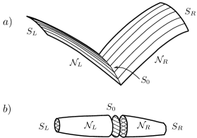
Figure 1: a) A double null sheet in 2+1 dimensional spacetime. b) In 3+1 dimensional spacetime ${\cal N}$ is a 3-manifold consisting of two solid cylinders joined on a disk, here shown without regard to their embedding in spacetime.

Nevertheless a constraint free canonical theory was not constructed, for two reasons: First, the Poisson brackets of the free initial data were unknown. Second, in order that ${\cal N}$ not enter its own future, implying intractable constraints on the otherwise free initial data, the generators must not cross at interior points of ${\cal N}$ Wald. (1984). But excluding such crossings itself seemed to require intractable conditions on the data. Here a Poisson bracket on free data corresponding to the Hilbert action is presented, and a simple way to avoid caustics and generator crossings is pointed out.

The resulting framework seems ideal for attempting a semi-classical proof of the Bousso entropy bound Bekenstein (1981); ’t Hooft (1993); Susskind (1995); Bousso (1999) in the vacuum gravity case, since a branch ${\cal N}_{A}$ ($A=L\ \mbox{or}\ R$) of ${\cal N}$ is a “light sheet” in the terminology of Bousso Bousso (1999) provided the generators are not diverging at $S_{0}$.

Canonical GR using constrained data on double null sheets has been developed by several authors Torre (1986); Goldberg et al. (1992); Goldberg and Soteriou (1995); d’Inverno et al. (2006). Presumably the present Poisson brackets can be interpreted as Dirac brackets in those frameworks. Results on the brackets of part of the free data are given in Refs. Goldberg and Soteriou (1995); Gambini and Restuccia (1978). Reference Gambini and Restuccia (1978) gives perturbation series in Newton’s constant for the brackets of free data living on the bulk of ${\cal N}$ consistent with the present work, but no brackets of the surface data on $S_{0}$. Reference Goldberg and Soteriou (1995) presents distinct free data on the bulk of ${\cal N}$, which are claimed to form a canonically conjugate pair on the basis of a machine calculation of Dirac brackets. It would be interesting to see if they are conjugate according to the bracket obtained here.

A special chart $(v_{A},\theta^{1},\theta^{2})$ will be used on each branch ${\cal N}_{A}$ of ${\cal N}$, with $v_{A}$ a parameter along the generators and $\theta^{a}$ ($a=1,2$) constant along these. Since $\partial_{v_{A}}$ is tangent to the generators it is null and normal to ${\cal N}_{A}$. The line element on ${\cal N}_{A}$ thus takes the form

$$ds^{2}=h_{ab}d\theta^{a}d\theta^{b},$$ (1)

with no $dv$ terms. $v_{A}$ is taken proportional to the square root of $\rho\equiv\sqrt{\det h}$, the area density in $\theta$ coordinates on 2D cross sections of ${\cal N}_{A}$, and normalized to $1$ at $S_{0}$. Thus $\rho=\rho_{0}(\theta^{1},\theta^{2})v_{A}^{2}$, with $\rho_{0}$ the area density on $S_{0}$. Any affine parameter $\eta$ on the generators is related to $v$ by Reisenberger (2007)

$$0=R[\partial_{v},\partial_{v}]=\frac{2}{v}\frac{d}{dv}\ln\Big{|}\frac{d\eta}{dv}\Big{|}+\frac{1}{4}\partial_{v}e_{ab}\partial_{v}e^{ab},$$ (2)

a vacuum Einstein equation equivalent to the “focusing equation” (9.2.32 in Wald. (1984)). Here $e_{ab}=h_{ab}/\rho$, a unit determinant, symmetric $2\times 2$ matrix.

At caustic points $v^{2}\equiv\rho/\rho_{0}$ vanishes, so the caustic free ${\cal N}$ are represented by initial data on coordinate domains in which $v>0$. In the absence of caustics generators can still cross on ${\cal N}$ but the crossing points can be “unidentified”: A spacetime which is locally isometric to a neighborhood of ${\cal N}$, but in which the generators do not cross, may be constructed by pulling the metric of the original spacetime back to the normal bundle of $S_{0}$ using the exponential map (Ref. Reisenberger (2007), Appendix B). The exclusion of caustics and crossings thus requiers no restriction on the data at $v>0$. In particular it does not restrict the scope of the present work to weak fields.

Since ${\cal N}_{A}$ is caustic free $d\theta^{1}\wedge d\theta^{2}$ is degenerate only along generators. $(v_{A},\theta^{1},\theta^{2})$ is thus a good chart provided $dv_{A}\neq 0$ on the generators. For smooth $S_{0}$, in a smooth vacuum solution, this is so if the generators are converging everywhere on $S_{0}$ ($v$ decreasing away from $S_{0}$), since by the focusing equation (2) $v$ continues to decrease until a caustic is reached, and also if the generators are diverging everywhere on $S_{0}$ but are truncated before they begin to reconverge. In these cases $e_{ab}$ induced by the spacetime geometry is smooth in $v$ and $\theta^{a}$. Conversely, if (A) $v$ is not strictly constant on a generator, and (B) $e_{ab}$ is smooth in $v$, then by (2) $dv\neq 0$ along the generator. The initial data will satisfy conditions A and B on all generators, ensuring that $(v,\theta^{1},\theta^{2})$ is a good chart.

Sachs Sachs (1962) showed (modulo convergence issues) that $e_{ab}$, specified on ${\cal N}$ as a function of an affine parameter on the generators, together with additional data on $S_{0}$, is free initial data determining the geometry of a spacetime region to the future of ${\cal N}$. Here we assume that any Sachs data without caustics determines a unique maximal Cauchy development $D[{\cal N}]$ of all of ${\cal N}$, and that if the data depend smoothly on a parameter the solution does as well. Existence, uniqueness, and smooth dependence on parameters have been proved rigorously in a neighborhood of $S_{0}$ Rendall (1990).

We will use similar data, including $e_{ab}$, given on ${\cal N}$ as a smooth function of $v$; and $\rho_{0}$, $\lambda=-\ln|n_{L}\cdot n_{R}|$, and

$$\tau_{a}=\frac{n_{L}\cdot\nabla_{a}n_{R}-n_{R}\cdot\nabla_{a}n_{L}}{n_{L}\cdot n_{R}}$$ (3)

specified on $S_{0}$. [Here $n_{A}=\partial_{v_{A}}$ is the tangent to the generators of ${\cal N}_{A}$, and inner products ($\cdot$) are evaluated using the spacetime metric.] $v_{A}$ ranges from $1$ on $S_{0}$ to $\bar{v}_{A}(\theta)$ on $S_{A}$. $\bar{v}_{A}(\theta)$, which is another datum, is required to be $>0$ and $\neq 1$. The data are smooth functions of the $\theta^{a}$, which range over the unit disk $(\theta^{1})^{2}+(\theta^{2})^{2}\leq 1$. Any valuation of these data determine, via (2), Sachs data free of caustics and thus, according to our asumptions, a solution to GR unique up to diffeomorphisms Reisenberger (2007).

However, because ${\cal N}$ has a boundary, not all infinitesimal diffeomorphisms are degeneracy vectors of the symplectic 2-form on ${\cal N}$ Reisenberger (2007). Two further data on $S_{0}$, $s^{m}_{L}$ and $s^{i}_{R}$, measure diffeomorphisms which are non-gauge in this sense. $y_{A}^{k}=s_{A}^{k}(\theta)$ is the position of the endpoint on $S_{A}\subset\partial{\cal N}$ of the generator $(\theta^{1},\theta^{2})$, in a fixed chart $y_{A}$ on $S_{A}$. Since $s_{A}$ may be varied independently of the other data by diffeomorphisms the complete data set is still free. We shall return to the question of the significance of the $s_{A}$.

In sum, the data consist of 10 real $C^{\infty}$ functions, $\rho_{0}$, $\lambda$, $\tau_{a}$, $\bar{v}_{A}$, and $s_{A}^{k}$, on the unit 2-disk with $\bar{v}_{A}>0$ and $\neq 1$, and two $C^{\infty}$, real, symmetric, unimodular $2\times 2$ matrix valued functions ($e_{ab}$ on ${\cal N}_{L}$ and ${\cal N}_{R}$) on the domains $\{(\theta^{1})^{2}+(\theta^{2})^{2}\leq 1,\min(1,\bar{v}_{A}(\theta))\leq v_{A}\leq\max(1,\bar{v}_{A}(\theta))\}$, $A=L,R$ which match at $v_{L}=v_{R}=1$ (i.e. on $S_{0}$). Our phase space is the space of valuations of these data.

An alternative representation of $e_{ab}$ can be obtained by expressing the degenerate line element (1) on ${\cal N}$ in terms of the complex coordinate $z=\theta^{1}+i\theta^{2}$:

$$ds^{2} = h_{ab}d\theta^{a}d\theta^{b}$$ (4)

$$= \rho(1-\mu\bar{\mu})^{-1}[dz+\mu d\bar{z}][d\bar{z}+\bar{\mu}dz],$$

with $\mu$ a complex number valued field of modulus less than 1 (sometimes called the Beltrami differential). $\mu$ encodes the two real degrees of freedom of $e_{ab}=h_{ab}/\rho$. This parametrization of $e_{ab}$ also works when $e_{ab}$ is not real, but then $\mu$ and $\bar{\mu}$ are no longer complex conjugates.

Finding the Poisson bracket on initial data by inverting the (gauge fixed) symplectic 2-form, or other conventional approaches, turns out to be difficult. But what is ultimately required of the bracket is that it gives the correct Poisson brackets for observables. We shall content ourselves with finding a bracket that satisfies this criterion. Observables will be defined as diffeomorphism invariant functionals of the metric $F[g]$ with $C^{\infty}$ functional derivatives $\delta F/\delta g_{\mu\nu}$ of compact support contained in the interior of the Cauchy development $D[{\cal N}]$. The Poisson brackets of these observables may be defined via Peierls’ Peierls (1952) covariant formula in terms of the action and Green’s functions Reisenberger (2007).

To match the Peierls bracket on observables $\{\cdot,\cdot\}_{\bullet}$ need only be almost inverse to the symplectic 2-form $\omega_{\cal N}$ on ${\cal N}$. Specifically, let $g$ be a metric satisfying the field equations and let $L^{0}_{g}$ be the space of perturbations of the metric that satisfy the field equations linearized about $g$ and vanish in a neighborhood of $\partial{\cal N}$. Then $\{\cdot,\cdot\}_{\bullet}$ matches the Peierls bracket on observables (at $g$) if

$$\delta\varphi=\omega_{\cal N}[\{\varphi,\cdot\}_{\bullet},\delta]\ \ \ \forall\>\delta\in L_{g}^{0}.$$ (5)

for all integrals, $\varphi$, of initial data against smooth test functions on ${\cal N}$ that vanish in a neighborhood of $\partial{\cal N}$ Reisenberger (2007).

We will use the symplectic 2-form of the Hilbert action, and we will require $\{\cdot,\cdot\}_{\bullet}$ to be causal: data at $p\in{\cal N}$ must commute with data outside the causal domain of influence of $p$, domain which on ${\cal N}$ reduces to just the generator(s) through $p$ Reisenberger (2007). Then $\omega_{\cal N}[\{\varphi,\cdot\}_{\bullet},\delta]$ in (5) can be expressed in terms of the initial data as $\Omega_{\cal N}[\{\varphi,\cdot\}_{\bullet},\delta]$ where $\Omega_{\cal N}=\Omega_{L}+\Omega_{R}$ with Reisenberger (2007)

$$16\pi G\Omega_{A}[\delta_{1},\delta_{2}] = \int_{S_{0}}d^{2}\theta\Big{\{}\delta_{1}\lambda\delta_{2}\rho_{0}+\delta_{1}\tilde{\tau}_{A\,k}\delta_{2}s_{A}^{k}$$ (6)

$$+\frac{1}{4}\delta_{1}^{y}\rho_{0}\partial_{v}e_{ab}\delta^{y}_{2}e^{ab}$$

$$+\frac{1}{2}\rho_{0}\int_{1}^{\bar{v}}v^{2}\delta^{\circ}_{1}e^{ab}\partial_{v}\delta^{\circ}_{2}e_{ab}dv\>\Big{\}}$$

$$-(1\leftrightarrow 2).$$

Here $\tilde{\tau}_{R\,i}dy_{R}^{i}=\rho_{0}[d\lambda-\tau]$ and $\tilde{\tau}_{L\,m}dy_{L}^{m}=\rho_{0}[d\lambda+\tau]$; $\delta^{y}=\delta-{\pounds}_{\xi_{\perp}}$, where $\xi_{\perp}=\delta s_{A}^{k}\partial_{y_{A}^{k}}$ and the partial derivative $\partial_{y_{A}^{k}}$ is taken at constant $v$; and $\delta^{\circ}=\delta^{y}-\frac{1}{2}\delta^{y}\ln\rho_{0}\,v\partial_{v}$. In calculating (6) no boundary terms were added to the Hilbert action because the Peierls bracket, which determines the brackets of observables, is unaffected by such terms. Equation (6) is consistent with Epp (1995).

Equation (5) does not determine the bracket uniquely, nor does it guarantee that it satisfies the Jacobi relations. Here a unique Poisson bracket is obtained by defining a set $C$ of variations of the data containing those corresponding to spacetime metric variations in $L_{g}^{0}$ and imposing

$$\delta\varphi=\Omega_{\cal N}[\{\varphi,\cdot\}_{\bullet},\delta]\ \ \ \forall\>\delta\in C\ \ \ \mbox{and}\ \ \ \{\varphi,\cdot\}_{\bullet}\in C,$$

(7)

for all $\varphi$ obtained by smearing data with any $C^{\infty}$ test function on ${\cal N}$ or $S_{0}$. The first condition ensures agreement with the Peierls bracket; the second that the Jacobi relations hold.

$C$ consists of all complex variations $\delta$ of the data such that (A) $\delta\bar{\mu}$ is smooth on ${\cal N}$ while $\delta\mu$ is smooth on ${\cal N}_{L}-S_{0}$, ${\cal N}_{R}-S_{0}$, and $S_{0}$, with possible jump dicontinuities between them, and (B) $\delta$ leaves invariant on $S_{A}$ both $\rho_{A}$, the area density in the $y_{A}$ chart, and $\mu_{A}$, the Beltrami differential in the complex chart $y^{1}_{A}+iy^{2}_{A}$. ($\delta\bar{\mu}_{A}$ need not vanish on $S_{A}$.)

The use of the space $C$ of complex perturbations on the real phase space is strange but seems difficult to avoid. Note however that all hamiltonian vectors defined by the $\bullet$ bracket satisfying (7) preserve the reality of observables, and of the metric on the interior of $D[{\cal N}]$.

Because of the identity

$$\tilde{\tau}_{R\,i}\partial_{a}s_{R}^{i}+\tilde{\tau}_{L\,m}\partial_{a}s_{L}^{m}=2\rho_{0}\partial_{a}\lambda$$ (8)

$\Omega_{\cal N}$ is degenerate with respect to variations of the data due to diffeomorphisms of the $\theta$ chart on $S_{0}$. This degeneracy can be removed by extending the phase space by making $\tilde{\tau}_{R}$ and $\tilde{\tau}_{L}$ independent, and treating (8) as a constraint (which generates diffeomorphisms of $\theta$ Reisenberger (2007)). Then (7) defines the $\bullet$ brackets of the data uniquely as two point distributions on $S_{0}$ and ${\cal N}$.

[A description without any constraint may be obtained by eliminating $\tilde{\tau}_{L}$ via (8), and $s_{L}$ via the gauge fixing $\theta=y_{L}$. The Dirac brackets of the remaining data are then identical to their extended phase space $\bullet$ brackets Reisenberger (2007).]

Solving (7) by a procedure like that of Reisenberger (2007) yields:

$$\{\rho_{0}(\bm{\theta}_{1}),\lambda(\bm{\theta}_{2})\}_{\bullet}=8\pi G\delta^{2}(\bm{\theta}_{2}-\bm{\theta}_{1}),$$ (9)

$$\{s_{A}^{i}(\bm{\theta}_{1}),\tilde{\tau}_{B\,j}(\bm{\theta}_{2})\}_{\bullet}=16\pi G\delta_{AB}\delta_{j}^{i}\delta^{2}(\bm{\theta}_{2}-\bm{\theta}_{1}),$$ (10)

and $s_{A}$ and $\rho_{0}$ commute with all other data.

The brackets between $\tilde{\tau}_{R}$, $\tilde{\tau}_{L}$, and $\lambda$ are

$$\{\lambda(\bm{\theta}_{1}),\lambda(\bm{\theta}_{2})\}_{\bullet}=0,$$ (11)

$$\{\lambda(\bm{\theta}),\tau_{R}[f]\}_{\bullet} = 8\pi G\Big{[}\frac{{\pounds}_{f}\mu}{(1-\mu\bar{\mu})^{2}}(\partial_{v_{R}}\bar{\mu}-\partial_{v_{L}}\bar{\mu})\Big{]}_{\bm{\theta}},\qquad$$

$$\{\tau_{R}[f_{1}],\tau_{R}[f_{2}]\}_{\bullet} = -16\pi G\int_{S_{0}}\frac{1}{(1-\mu\bar{\mu})^{2}}{\pounds}_{f_{1}}\mu(\epsilon{\pounds}_{f_{2}}\bar{\mu}$$ (13)

$$-{\pounds}_{f_{2}}\epsilon\partial_{v_{R}}\bar{\mu})-(1\leftrightarrow 2),$$

$$\{\tau_{R}[f],\tau_{L}[g]\}_{\bullet} = 16\pi G\int_{S_{0}}\frac{1}{(1-\mu\bar{\mu})^{2}}{\pounds}_{f}\mu(\epsilon{\pounds}_{g}\bar{\mu}$$ (14)

$$-{\pounds}_{g}\epsilon\partial_{v_{L}}\bar{\mu})-(f,R\leftrightarrow g,L),$$

the rest being obtainable from these by exchanging $L$ and $R$. $\epsilon$ is the area form $\rho_{0}d\theta^{1}\wedge d\theta^{2}$, $\tau_{R}[f]=\int_{S_{0}}\tilde{\tau}_{R\,i}f^{i}d^{2}\theta$ with $f^{i}(\theta)$ test functions independent of the data, and $\tau_{L}[g]$ is defined similarly in terms of test functions $g^{m}$. $f^{i}$ and $g^{m}$ define vector fields $f=f^{i}\partial_{y_{R}^{i}}$ and $g=g^{m}\partial_{y_{L}^{m}}$, and thus Lie derivatives. The only unusual one is

$${\pounds}_{f}\mu=f^{z}\partial_{z}\mu+f^{\bar{z}}\partial_{\bar{z}}\mu-\mu[\partial_{z}f^{z}-\partial_{\bar{z}}f^{\bar{z}}]-\mu^{2}\partial_{z}f^{\bar{z}}+\partial_{\bar{z}}f^{z}$$

The brackets between $\mu$ and $\bar{\mu}$ are as follows: If ${\mathbf{1}},{\mathbf{2}}$ denote the $(v,\theta)$ coordinates of any pair of points on ${\cal N}$

$$0=\{\mu({\mathbf{1}}),\mu({\mathbf{2}})\}_{\bullet}=\{\bar{\mu}({\mathbf{1}}),\bar{\mu}({\mathbf{2}})\}_{\bullet}.$$ (15)

When ${\mathbf{1}}$ and ${\mathbf{2}}$ do not lie on the same branch also $\{\mu({\mathbf{1}}),\bar{\mu}({\mathbf{2}})\}_{\bullet}=0$, but if ${\mathbf{1}}$ and ${\mathbf{2}}$ do lie on the same branch, ${\cal N}_{A}$, then

$$\{\mu({\mathbf{1}}),\bar{\mu}({\mathbf{2}})\}_{\bullet} = 4\pi G\,\frac{1}{\rho_{0}}\delta^{2}(\bm{\theta}_{2}-\bm{\theta}_{1})\,H({\mathbf{1}},{\mathbf{2}})\Big{[}\frac{1-\mu\bar{\mu}}{v_{A}}\Big{]}_{\mathbf{1}}$$

$$\times\Big{[}\frac{1-\mu\bar{\mu}}{v_{A}}\Big{]}_{\mathbf{2}}\>e^{\int_{\mathbf{1}}^{\mathbf{2}}(\bar{\mu}d\mu-\mu d\bar{\mu})/(1-\mu\bar{\mu})},$$

where if ${\mathbf{1}}$ and ${\mathbf{2}}$ lie on the same generator the integral runs along the generator segment from ${\mathbf{1}}$ to ${\mathbf{2}}$, and $H$ is a step function equal to $1$ if ${\mathbf{1}}$ lies on or between $S_{0}$ and ${\mathbf{2}}$, and $0$ otherwise. Here and elsewhere the coefficient of $\delta^{2}(\bm{\theta}_{2}-\bm{\theta}_{1})$ is extended continuously to $\bm{\theta}_{2}\neq\bm{\theta}_{1}$.

There remain the brackets of $\mu$ and $\bar{\mu}$ with the $S_{0}$ data $\lambda$, $\tilde{\tau}_{R}$, and $\tilde{\tau}_{L}$. For ${\mathbf{1}}$ on ${\cal N}_{R}-S_{0}$ (i.e. $v_{R\,1}\neq 1$)

$$\{\mu({\mathbf{1}}),\lambda({\bm{\theta}_{2}})\}_{\bullet}=4\pi G\frac{1}{\rho_{0}}\delta^{2}(\bm{\theta}_{2}-\bm{\theta}_{1})[v_{R}\partial_{v_{R}}\mu]_{\mathbf{1}},$$ (17)

$$\{\mu({\mathbf{1}}),\tau_{R}[f]\}_{\bullet}=8\pi G\Big{[}2{\pounds}_{f}\mu-\frac{{\pounds}_{f}\rho_{0}}{\rho_{0}}v_{R}\partial_{v_{R}}\mu\Big{]}_{\mathbf{1}},$$ (18)

$$\{\mu({\mathbf{1}}),\tau_{L}[g]\}_{\bullet}=0,$$ (19)

while for ${\mathbf{1}}$ on $S_{0}$

$$\{\mu({\mathbf{1}}),\lambda({\mathbf{2}})\}_{\bullet}=0,$$ (20)

$$\{\mu({\mathbf{1}}),\tau_{R}[f]\}_{\bullet}=8\pi G[{\pounds}_{f}\mu]_{\mathbf{1}},$$ (21)

$$\{\mu({\mathbf{1}}),\tau_{L}[g]\}_{\bullet}=8\pi G[{\pounds}_{g}\mu]_{\mathbf{1}}.$$ (22)

On the other hand, for all ${\mathbf{1}}\in{\cal N}_{R}$ (including ${\mathbf{1}}\in S_{0}$)

$$\{\bar{\mu}({\mathbf{1}}),\lambda(\bm{\theta}_{2})\}_{\bullet} = 4\pi G\frac{1}{\rho_{0}}\delta^{2}(\bm{\theta}_{2}-\bm{\theta}_{1})\Big{[}(v_{R}\partial_{v_{R}}\bar{\mu})_{\mathbf{1}}$$

$$+\Big{(}\frac{1}{v_{R}}\Big{)}_{\mathbf{1}}e^{2\int_{\mathbf{1}}^{\mathbf{2}}(\mu d\bar{\mu})/(1-\mu\bar{\mu})}(\partial_{v_{L}}\bar{\mu})_{\mathbf{2}}\Big{]},$$

$$\{\bar{\mu}({\mathbf{1}}),\tau_{R}[f]\}_{\bullet} = 8\pi G\Big{[}\Big{(}2{\pounds}_{f}\bar{\mu}-\frac{{\pounds}_{f}\rho_{0}}{\rho_{0}}v_{R}\partial_{v_{R}}\bar{\mu}\Big{)}_{\mathbf{1}}$$

$$-({\pounds}_{f}\bar{\mu})_{{\mathbf{1}}_{0}}\Big{(}\frac{1}{v_{R}}\Big{)}_{\mathbf{1}}e^{-2\int_{{\mathbf{1}}_{0}}^{\mathbf{1}}(\mu d\bar{\mu})/(1-\mu\bar{\mu})}\Big{]},$$

$$\{\bar{\mu}({\mathbf{1}}),\tau_{L}[g]\}_{\bullet} = 8\pi G\Big{[}{\pounds}_{g}\bar{\mu}-\frac{{\pounds}_{g}\rho_{0}}{\rho_{0}}\partial_{v_{L}}\bar{\mu}\Big{]}_{{\mathbf{1}}_{0}}$$ (25)

$$\times\Big{(}\frac{1}{v_{R}}\Big{)}_{\mathbf{1}}e^{-2\int_{{\mathbf{1}}_{0}}^{\mathbf{1}}(\mu d\bar{\mu})/(1-\mu\bar{\mu})},$$

where ${\mathbf{1}}_{0}\in S_{0}$ is the base point of the generator through ${\mathbf{1}}$. Exchanging $L$ and $R$ in (17)–(25) gives the corresponding brackets for ${\mathbf{1}}$ on ${\cal N}_{L}$.

Finally, the brackets of $\bar{v}_{A}$ follow from the preceeding brackets and the fact that, by (7), $\rho_{A}=\rho_{0}\bar{v}_{A}^{2}|\det\partial_{a}s_{A}^{k}|^{-1}$ at given $y_{A}$ commutes with everything. Alternatively, $\bar{v}_{A}(\theta)$ may be replaced as a phase coordinate by $\rho_{A}(y_{A})$.

Direct calculations confirm that these expressions for the brackets satisfy the Jacobi relations, that they are invariant under diffeomorphisms of the (arbitrarily chosen) coordinates $y_{R}^{i}$, $y_{L}^{m}$ and $\theta^{a}$ Reisenberger (2007), and that the constraint (8) generates diffeomorphisms of the $\theta^{a}$ Reisenberger (2007).

Strangely, the brackets do not preserve the reality of $e_{ab}$, i.e. the complex conjugacy of $\mu$ and $\bar{\mu}$. An analytic functional $F$ of the data is real on real data iff it equals $\bar{F}$, its formal complex conjugate, obtained by exchanging $\mu$ and $\bar{\mu}$, leaving the $S_{0}$ data untouched, and replacing numerical coefficients by their complex conjugates. $\{F,\cdot\}_{\bullet}$ preserves the reality of the data for all formally real $F$ iff the bracket itself is real in the sense that it equals the formal complex conjugate bracket $\{\varphi,\chi\}_{\bullet c.c.}\equiv\overline{\{\bar{\varphi},\bar{\chi}\}}_{\bullet}$. But this is not so: $\overline{\{\mu({\mathbf{1}}),\bar{\mu}({\mathbf{2}})\}_{\bullet}}\neq\{\bar{\mu}({\mathbf{1}}),\mu({\mathbf{2}})\}_{\bullet}$. Nevertheless, on observables the bracket is real, as it reproduces the real Peierls bracket. In fact, one may resolve the $\bullet$ bracket into (formal) real and imaginary parts, $\{\cdot,\cdot\}_{\bullet}=\{\cdot,\cdot\}_{R}+i\{\cdot,\cdot\}_{I}$, and one finds that

$$\{\cdot,\cdot\}_{I} = \frac{i}{8\pi G}\sum_{A=L,R}\int_{S_{A}}\epsilon\frac{1}{(1-\mu_{A}\bar{\mu}_{A})^{2}}[\{\cdot,\bar{\mu}_{A}\}_{\bullet}\overline{\{\bar{\mu}_{A},\bar{\cdot}\}}_{\bullet}$$ (26)

$$-\overline{\{\bar{\cdot},\bar{\mu}_{A}\}}_{\bullet}\{\bar{\mu}_{A},\cdot\}_{\bullet}].$$

In agreement with causality, $\{\bar{\mu}_{A}(q),\cdot\}_{\bullet}$ for $q\in S_{A}$ is a gravitational wave pulse that skims along ${\cal N}_{A}$ without entering the interior of $D[{\cal N}]$. It does not affect the metric there (Ref. Reisenberger (2007), Appendix C), so neither does $\{\phi,\cdot\}_{I}$ for any datum $\phi$.

$\{\cdot,\cdot\}_{R}$ is the pre-Poisson bracket $\{\cdot,\cdot\}_{\circ}$ of Reisenberger (2007), which does not satisfy the Jacobi relations, so the imaginary part (26) is necessary. One may reverse its sign, but given the action there seems to be little, if any, further freedom in the bracket. Adding boundary terms to the action, which does not affect the Peierls bracket, might alter $\{\cdot,\cdot\}_{\bullet}$.

The data $s_{A}$, $A=L,R$ seem unphysical as they do not affect the geometry of the solution, yet they participate in the Poisson bracket. In fact $s_{A}$ may be replaced almost entirely by $\mu_{A}$, which commutes with everything. $\mu$ and $\mu_{A}$ together determine $s_{A}:\theta\mapsto y_{A}$ up to the three parameter group of conformal maps of the unit disk to itself. Moreover $\mu_{A}$ can always be set to zero by a suitable choice of $y_{A}$ chart. The remaing three degrees of freedom in $s_{A}$ are determined by the boundary values of $s_{A}$ on $\partial S_{0}$, which commute with all data on the interior of ${\cal N}$. Of course, were $S_{0}$ a 2-sphere instead of a disk no boundary values would be available to fix the conformal automorphisms.

$\rho_{0}$, $s_{L}$, $s_{R}$ and $\mu$ qualify as “configuration variables” since they form a maximal commuting set among functionals of the data. [We regard $\rho_{L}(y_{L})$ and $\rho_{R}(y_{R})$, which commute with everything, as fixed]. A quantization may thus be attempted in terms of wave functionals depending on $\rho_{0}$, $s_{L}$, $s_{R}$, and $\mu$, but annihilated by $\delta/\delta\bar{\mu}$.

References

• Sachs (1962) R. K. Sachs, J. Math. Phys. (N.Y.) 3, 908 (1962).
• Penrose (1980) R. Penrose, Gen. Relativ. Gravit. 12, 225 (1980), originally published in Aerospace Research Laboratories Report 63-56 edited by P. G. Bergmann, 1963.
• Bondi et al. (1962) H. Bondi, M. van der Burg, and A. Metzner, Proc. R. Soc. A 269, 21 (1962).
• Dautcourt (1963) G. Dautcourt, Ann. Physik. (Leipzig) 467, 302 (1963).
• Wald. (1984) R. M. Wald., General Relativity (University of Chicago Press, Chicago, 1984).
• Bekenstein (1981) J. D. Bekenstein, Phys. Rev. D 23, 287 (1981).
• ’t Hooft (1993) G. ’t Hooft (1993), eprint arXiv:gr-qc/9310026.
• Susskind (1995) L. Susskind, J. Math. Phys.(N.Y.) 36, 6377 (1995).
• Bousso (1999) R. Bousso, J. High Energy Phys. 07, 4 (1999).
• Torre (1986) C. G. Torre, Classical Quantum Gravity 3, 773 (1986).
• Goldberg et al. (1992) J. N. Goldberg, D. C. Robinson, and C. Soteriou, Classical Quantum Gravity 9, 1309 (1992).
• Goldberg and Soteriou (1995) J. N. Goldberg and C. Soteriou, Classical Quantum Gravity 12, 2779 (1995).
• d’Inverno et al. (2006) R. A. d’Inverno, P. Lambert, and J. A. Vickers, Classical Quantum Gravity 23, 4511 (2006).
• Gambini and Restuccia (1978) R. Gambini and A. Restuccia, Phys. Rev. D 17, 3150 (1978).
• Reisenberger (2007) M. P. Reisenberger (2007), eprint arXiv:gr-qc/0703134.
• Rendall (1990) A. D. Rendall, Proc. R. Soc. A 427, 221 (1990).
• Peierls (1952) R. E. Peierls, Proc. R. Soc. A 214, 143 (1952).
• Epp (1995) R. Epp (1995), eprint arXiv:gr-qc/9511060.