The signature of chromospheric heating in Ca II H spectra

Abstract

Context. The heating process that balances the solar chromospheric energy losses has not yet been determined. Conflicting views exist on the source of the energy and the influence of photospheric magnetic fields on chromospheric heating.

Aims. We analyze a 1-hour time series of cospatial Ca II H intensity spectra and photospheric polarimetric spectra around 630 nm to derive the signature of the chromospheric heating process in the spectra and to investigate its relation to photospheric magnetic fields. The data were taken in a quiet Sun area on disc center without strong magnetic activity.

Methods. We have derived several characteristic quantities of Ca II H to define the chromospheric atmosphere properties. We study the power of the Fourier transform at different wavelengths and the phase relations between them. We perform local thermodynamic equilibrium (LTE) inversions of the spectropolarimetric data to obtain the photospheric magnetic field, once including the Ca intensity spectra.

Results. We find that the emission in the Ca II H line core at locations without detectable photospheric polarization signal is due to waves that propagate in around 100 sec from low forming continuum layers in the line wing up to the line core. The phase differences of intensity oscillations at different wavelengths indicate standing waves for $\nu<$ 2 mHz and propagating waves for higher frequencies. The waves steepen into shocks in the chromosphere. On average, shocks are both preceded and followed by intensity reductions. In field-free regions, the profiles show emission about half of the time. The correlation between wavelengths and the decorrelation time is significantly higher in the presence of magnetic fields than for field-free areas. The average Ca II H profile in the presence of magnetic fields contains emission features symmetric to the line core and an asymmetric contribution, where mainly the blue H2V emission peak is increased (shock signature).

Conclusions. We find that acoustic waves steepening into shocks are responsible for the emission in the Ca II H line core for locations without photospheric magnetic fields. We suggest using wavelengths in the line wing of Ca II H, where LTE still applies, to compare theoretical heating models with observations.

1 Introduction

The discovery of the flash spectrum of the sun in the late 19th century led astronomers to call this colorful layer of the solar atmosphere the chromosphere. Since the emission lines in the chromospheric spectra have to form in a hotter medium than the visible photosphere, the chromospheric temperature stratification and its heating process became the first challenge to our understanding of the outer solar atmosphere. The temperature rise in the chromosphere is a direct consequence of the rare (radiative) interactions in a low-density medium, where departure from LTE is significant. Including non-LTE is a key ingredient in all models of the outer solar atmosphere (Fontenla et al. 2006, and references therein).

The dominant heating mechanism in the chromosphere has been a matter of discussion in the last 60 years (Narain & Ulmschneider 1996). Biermann (1948) was one of the first to suggest that mechanical heating prevents the chromosphere from rapidly cooling down to below the photospheric temperature. Although the presence of waves in the solar atmosphere is well established, their importance for the chromospheric energy balance is under debate. Rammacher & Ulmschneider (1992), for instance, modeled wave propagation in the solar atmosphere using a 1-D code with various initial velocity fields. They obtained 3-min like oscillations using a short-period driver with 40 seconds cadence by the process of shock overtaking or shock merging. Their results depended slightly on the exact shape and periodicity of the initial wave field, supposedly present from the interference of the acoustic waves permeating the solar photosphere. Contrary to that, Fossum & Carlsson (2005, 2006) have recently suggested that the acoustic wave power is not sufficient to supply chromospheric energy losses (see also Wedemeyer-Böhm et al. 2007).

The role of magnetic fields for the chromospheric energy balance is also unclear. The strong flux concentrations at the boundaries of (super)granules can be easily identified through their emission in chromospheric lines (“chromospheric network”), but the importance of weaker magnetic fields for the chromosphere is unknown, as well as why there is permanent enhanced emission in the network. Kalkofen (1996) suggest collisions between flux concentrations and granules as the initial driver of the oscillations, which would only be an indirect influence. Rezaei et al. (2007) decomposed average Ca profiles into a non-heated, a non-magnetically, and a magnetically heated component. They conclude that the magnetic heating depends on the photospheric magnetic flux to some extent, but in total is weaker than the non-magnetically heating.

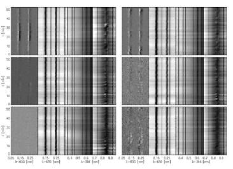
Figure 1: Six examples of the temporal evolution at fixed positions along the slit. Time is increasing from bottom to top for each example. Right to left in each image: Ca spectra; intensity and Stokes V spectra at 630 nm. The Ca spectra are displayed in two separately scaled parts, to enhance the visibility of the line core.

Few strong spectral lines are suited to observe the chromosphere from the ground (Ca II H and K, the Ca II triplet around 850 nm, H$\alpha$, Helium 1083 nm). Most of these lines are very broad and deep, often observed using broad-band filters with very limited spectral resolution. From space, additional low-forming emission lines and continuum windows are accessible (e.g., in the UV at 1600 nm; Fossum & Carlsson 2006; de Wijn et al. 2007). Hence, the analysis of the chromosphere is based on either high-resolution spectra with low temporal cadence and a limited field-of-view (FOV), or on two-dimensional data with large FOVs and poor spectral resolution. Only recently, 2-D observations with high spectral resolution have been carried out on spectral lines in the chromosphere and the upper photosphere (Vecchio et al. 2007, using IBIS).

Several approaches have been taken in simulations to examine the mechanical heating and the shock propagation in the upper solar atmosphere: 1-D dynamical simulations of waves in the solar atmosphere (e.g. Rammacher & Ulmschneider 1992), and 2-D and 3-D simulations of the solar atmosphere without an artificial excitation of waves (e.g. Wedemeyer et al. 2004). Whereas temporally and spatially averaged spectra can be reproduced by static temperature stratifications with a temperature minimum between photosphere and chromosphere (Vernazza et al. 1981, and its variants), the dynamical evolution of the chromosphere leads to various physical states and even more observed profile shapes (due to the integration across different physical states along the line-of-sight in a single profile). All numerical simulations predict cool episodes in the chromosphere which is in contradiction with a full-time hot chromosphere. The discrepancy between spectra with high spatial and temporal resolution from observations or simulations and the classical chromospheric models has been a matter of strong debate (Fontenla et al. 2007).

One of the few examples of a successful combination of observations and theory is the interpretation of the bright points or bright grains seen in the Ca II H and K lines. These grains appear as short-lived small-scale intensity enhancements in the H and K line cores all over the solar surface, in internetwork areas seemingly devoid of magnetic fields, but also on the locations of network fields at the boundaries of supergranules. The grains can repeat a few times with a cadence of around 200 sec (e.g., von Uexküll & Kneer 1995), but the process is stochastic. Rutten & Uitenbroek (1991) concluded that H_2V grains, where the blue emission peak of the Ca II H line is increased, and the less frequent H_2R grains are produced by the collision of p-mode oscillations, an event inside the photospheric wave field. The direct relation of the grains to the photosphere was later proven by Carlsson & Stein (1997). They successfully reproduced the temporal evolution of observed Ca II H spectra in a dynamical 1-D simulation, employing a photospheric “piston” with velocities taken from a line blend in the wing of Ca II H. Their calculations have, however, generally yielded shocks that are too strong and temperatures that are too extreme to seem realistic for the Sun, but this is presumably due to the 1-D ansatz.

In this contribution, we used data from the POLIS instrument (Beck et al. 2005b) to study the signature of the chromospheric heating process in Ca II H spectra. The polarimetric channel of POLIS at 630 nm allowed us to localize photospheric magnetic fields, removing one of the big unknowns when analyzing Ca intensity spectra or filtergrams. Using the cospatial and cotemporal intensity spectra in the Ca II H line and vector-polarimetric spectra at 630 nm (Sect. 2), we analyzed a 1-hr time series on both the statistical properties of the chromospheric emission and its relation to photospheric fields (Sect. 3). We especially investigated the variation of properties with wavelength in the wing of the Ca II H line, which samples the layers from the photosphere to the line core in the chromosphere. We divided the FOV into three subfields: emission with and without strong photospheric magnetic field and very quiet regions. We compared the average profiles of the three regions, assuming them to contain different heating contributions (no heating, purely acoustic, acoustic and magnetic heating) in Sect. 4. We then studied the evolution of individual and spatially averaged profiles connected to shock events (Sect. 5). The findings are summarized and discussed in Sect. 6.

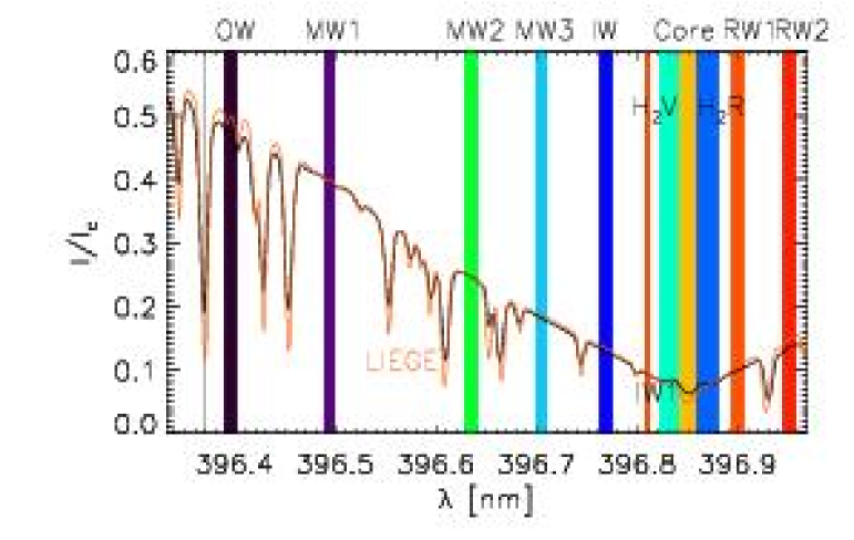
Figure 2: Average Ca spectrum with the wavelength bands for the derived intensities. Black line: average Ca spectrum. Orange line: LIEGE atlas reference profile. The thin vertical line marks the spectral line at 396.38 nm.

Table 1: The wavelength bands defined in the line wing and line core.

name	shortcut	wavelength $\pm$ width [nm]
outer wing	OW	396.397 $\pm$ 0.005
middle wing 1	MW1	396.494 $\pm$ 0.005
middle wing 2	MW2	396.634 $\pm$ 0.005
middle wing 3	MW3	396.702 $\pm$ 0.005
inner wing	IW	396.766 $\pm$ 0.005
inner wing	IW1	396.807 $\pm$ 0.002
H2V		396.832 $\pm$ 0.012
Core		396.847 $\pm$ 0.007
H2R		396.856 $\pm$ 0.012
red wing 1	RW1	396.892 $\pm$ 0.005
red wing 2	RW2	396.950 $\pm$ 0.005
H-index		396.848 $\pm$ 0.050

2 Observations, data reduction, and data alignment

We observed a quiet Sun area on disc center on 24 July 2006, from UT 08:11:50 until 09:06:44, with the POlarimetric LIttrow Spectrograph (POLIS, Beck et al. 2005b) at the German Vacuum Tower Telescope on Tenerife. There was no sign of significant magnetic activity near disc center on that day. The full data set consisted of a scan of 4 steps with 0$\aas@@fstack{\prime\prime}$5 step width that was repeated more than 150 times. The slit width corresponded to 0$\aas@@fstack{\prime\prime}$5, and the integration time per scan step was around 5 seconds. The Kiepenheuer-Institute adaptive optics system (von der Lühe et al. 2003), which was used to improve image quality, lost tracking after around 1 hour. For the present study, we thus selected only the first 150 repetitions of the scan for analysis.

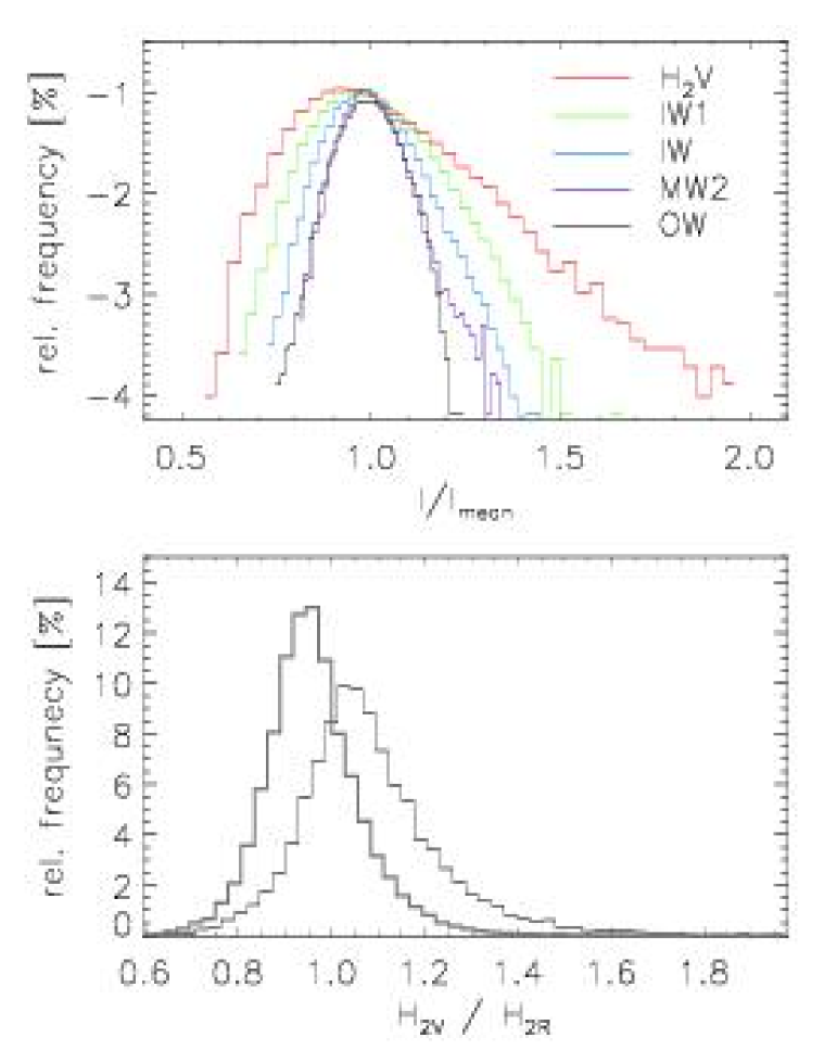
Figure 3: Top: Intensity histograms for some of the wavelength bands. The intensity map in each wavelength has been normalized to its mean value beforehand. Bottom: Ratio H_2V/H_2R using the wavelength bands (thick grey) or the peak intensities (thin black).

The spectra of both POLIS channels (blue, Ca II H 396.8 nm, intensity profiles; red, 630 nm, Stokes $IQUV$) were reduced with the usual flatfield and polarimetric calibration procedures (Beck et al. 2005a, b). The Ca spectra were additionally corrected for the transmission curve of the order-selecting interference filter in front of the camera. The Ca spectra were normalized afterwards to the LIEGE spectral atlas reference profile (Delbouille et al. 1973). For the Ca spectra, the wavelength scale of the LIEGE profile was adopted; for the red channel, the wavelength scale was set to have the line core of 630.15 (630.25) nm in the average profile of the full data set at a convective blueshift of -180 (-240) ms^-1. The intensity increase during the observations due to the rise of the Sun was removed separately in both channels by a fit of a straight line to average intensities along the slit.

Due to the differential refraction in the earth atmosphere (e.g. Reardon 2006), the spectra of the two POLIS channels were not fully cospatial and cotemporal. The spatial displacement of the two wavelengths perpendicular to the slit was of the order of 2^′′, given the date of the observations, the slit orientation, and the location of the first coelostat mirror (cf. Appendix A). Hence, only the first step in the blue channel was cospatial to the last of the four steps in the red channel in each scan. Discarding all steps without cospatial spectra, the data thus finally reduce to a time series of around 52 min duration with fixed slit and with around 21 seconds cadence, but in two wavelengths. The red channel was taken 21 seconds later than the blue. As no alignment in the direction perpendicular to the slit is possible (no data available), the data have been aligned only along the slit by cross-correlation of the tempo-spatial intensity maps. After alignment, a cospatial slit of 209 pixels with a sampling of 0$\aas@@fstack{\prime\prime}$29 per pixel remained.

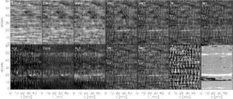
Figure 4: Spatio-temporal maps of continuum intensity in the red channel (top left), in the intensity bands defined in Table 1, LOS velocity of 630.25 nm (dark corresponds to blue shifts), and integrated signed Stokes $V$ signal (bottom right).

3 Data analysis & results

The data consists of the intensity profiles of the blue channel, and the Stokes vector measurements in the red channel. Figure 1 shows six examples of the temporal evolution of spectra at different locations along the slit during the full time series. These examples serve to show the kind of informations that can be extracted from the data set: the temporal evolution of the thermodynamics at several heights in the atmosphere from the blue channel, and the photospheric magnetic and velocity fields from the polarimetric red channel.

3.1 Ca II H spectra

Similar to Rezaei et al. (2007), we defined several wavelength bands in the Ca spectra, going from outermost wing across the line core to the red wing of the Ca spectrum (cf. Fig. 2). Table 1 contains the wavelength bands in detail. The bands were mainly choosen to encompass continuum windows, besides those in the Ca line core (H_2V, core, H_2R). Note that our definition is different from the one used in previous literature. The regions used for H_2V and H_2R in fact touch each other; the wavelength bands for the emission peaks thus include the left and right halves of the absorption core, respectively. As both core and emission peaks can show large spectral displacements (Fig. 1), we think they are covered better by this extended range. We also used the H-index as an emulated 1-Å-filter centered on the line core. In some methods employed to obtain information, e.g. Fourier power or correlation matrices, each wavelength of the Ca spectrum was used individually. For all Ca spectra with two reversals in the intensity profile, we determined the amplitude and location of the H_2V and H_2R emission peaks. We derived the line-core velocity of Fe I at 396.38 nm as a measure of the photospheric flow field. We chose this line because it is isolated, deep, and far separated from the Ca II H line core. As the line is contained in the Ca line wing, it is perfectly cospatial and cotemporal to the rest of the Ca spectrum.

The upper panel of Fig. 3 shows the intensity histograms in some of the wavelength bands. Two trends can be seen going from the wing towards the line core: the histograms become broader, and more and more asymmetric with an extended tail of high intensities. Leenaarts & Wedemeyer-Böhm (2005) obtained the intensity distribution at a wavelength of 396.74 nm from simulations with the Co⁵bold code, corresponding to the IW in the present paper. Comparing to their Fig. 2, we caution that the effects of degrading the (simulations’) spatial resolution is similar to moving in wavelength from, e.g, H_2V to IW1. Intensity histograms of filtergram observations then will be very sensitive to both the spatial resolution and the exact location and width of the filter used.

Rammacher (2005, R05) suggested using the ratio of H_2V/H_2R to determine the shape and amplitude of the acoustic power spectrum presumably heating the chromosphere. The lower panel of Fig. 3 shows the histograms of the ratio using the wavelength bands, or all locations, where a double reversal with two clear emission peaks was observed in the spectra. The two distributions are similar, centered around one, with an extended tail to high H_2V/H_2R ratios. Compared to R05, the distributions are much smoother without isolated peaks, and smaller maximal ratios (below 2). This could be due to the difference between the 1-D calculations employed by R05, which tend to generate strong shocks, and the 3-D solar atmosphere.

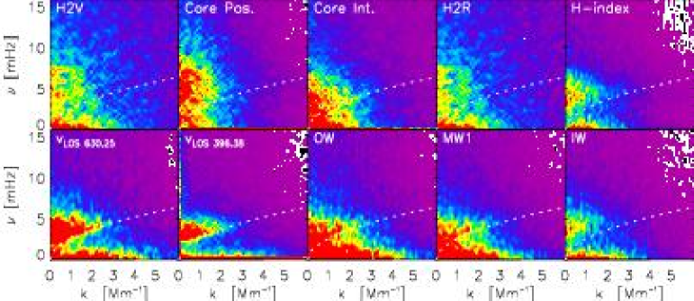
Figure 5: k-$\nu$-diagrams. Bottom row, left to right: line-of-sight velocity of 630.25 nm, same for 396.38 nm, outer, middle, inner wing. Top row: H_2V, position of Ca core derived from the location of minimum intensity, intensity of minimum, H_2R, H-index. The dashed line gives the fundamental mode of the p-mode oscillations ($\nu=\sqrt{g\cdot k}/2\pi$, with the solar surface gravity $g=273$ ms^-2).

3.2 630 nm spectra

The spectropolarimetric spectra of the red channel were inverted with the SIR code (Ruiz Cobo & del Toro Iniesta 1992; Ruiz Cobo 1998). The inversion scheme employed a single field-free component and straylight for profiles without clear polarization signal; otherwise, a two-component model of one magnetic atmosphere, one field-free component, and straylight were adopted. All quantities besides temperature were assumed to be constant with depth. As Fig. 4 shows, actually only few locations along the slit showed stronger polarization signals. This inversion used only the 630 nm spectra, and was performed in the full field of view.

The inversion was repeated for all time steps of 30 pixels along the slit (y$\sim 20^{\prime\prime}$ to 30^′′ in Fig. 4) including the Ca spectra, with identical settings to those before. The aim was to investigate whether an LTE inversion can still capture the propagation of waves and shocks in the lower atmospheric layers. Appendix B shows some examples of the observed and best-fit profiles of this inversion setup. From the satisfactory reproduction of the observed spectra – excluding the actual Ca line core and maybe the IW1 band – we conclude that the continuum bands defined should be accessible by an LTE inversion (cf. Owocki & Auer 1980, for the Ca II K wing). However, we refrain from using these inversion results at present before a rigid investigation of their reliability. The line-core velocities of the Fe I lines at 630.15 nm and 630.25 nm were determined as additional measurements of the photospheric velocity field. The velocity dispersion of the red channel of 0.7 kms^-1 per pixel is about two times smaller than in the blue channel, giving a better velocity resolution.

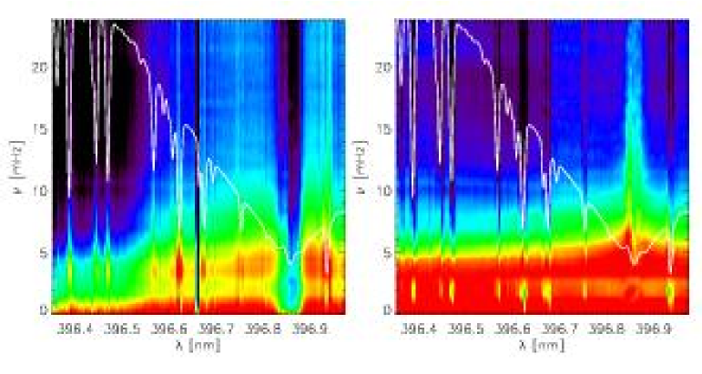
Figure 6: Power as function of wavelength and frequency, averaged along the slit. Left: normalized with P($\lambda,\nu$=0.3 mHz). Right: normalized with the power at 3 mHz, P($\lambda,\nu$=3 mHz).

3.3 Morphology of observed FOV

Figure 4 shows the temporal evolution of the intensity along the slit in the wavelength bands of Table 1. Passing from continuum wavelengths to the Ca line core, the structures visible change drastically. The tempo-spatial maps from continuum to MW1 are dominated by the structure and the temporal evolution of the granulation, leading to a mainly horizontally ($\equiv$temporal axis) oriented pattern of bright and dark stripes. For all other maps, the granulation signature is completely lost and exchanged by a vertically ($\equiv$spatial axis) oriented pattern of isolated (repeated) brightenings. The brightenings in H_2V or core last only shortly (20-60 sec) and extend over 2^′′ to 3^′′ along the slit. Many of the brightenings on locations without strong magnetic fields are repetitive with periods of 150 sec to 250 sec.

Four magnetic elements were intersected by the slit (y$\sim 12^{\prime\prime}$, 15^′′, 20^′′, 50^′′), which are seen all throughout the time series at approximately the same locations. Almost all locations that were inverted with a magnetic atmosphere belong to these four patches; they outline network fields ($B\sim 1.3$ kG, Fig. 25). Other locations only show transient weak polarization signals. Comparing the map of polarization signal (bottom right of Fig. 4) and that of, e.g., H_2V (bottom left), one can discriminate between three different types of locations in the FOV. Cospatial to strong photospheric fields, one finds a quasi-static intensity increase with less signatures of oscillations, and a small halo with higher intensity on the neighboring pixels. Contrary to the field-free locations, the oscillations on the field concentrations only modulate the emission, but do not lead to its disappearance, especially in the H_2R map. Close to fields (y$\sim 22^{\prime\prime}$ to $27^{\prime\prime}$ and $\sim 37^{\prime\prime}$ to $42^{\prime\prime}$), the periodic structure of the brightenings is most prominent (“caterpillar tracks”). In very quiet locations ($\sim 27^{\prime\prime}$ to $37^{\prime\prime}$), fewer and often non-repetitive brightenings can be found (t$\sim 20$ min, y$\sim 32^{\prime\prime}$).

3.4 Fourier analysis of Ca II H spectra

To quantify the properties of the intensity and velocity oscillations, we took the Fourier transform of the tempo-spatial maps. We try to isolate the general properties of the oscillations in the full FOV, and later investigate differences between locations with or without field, or in the very quiet area, by using spatially resolved information.

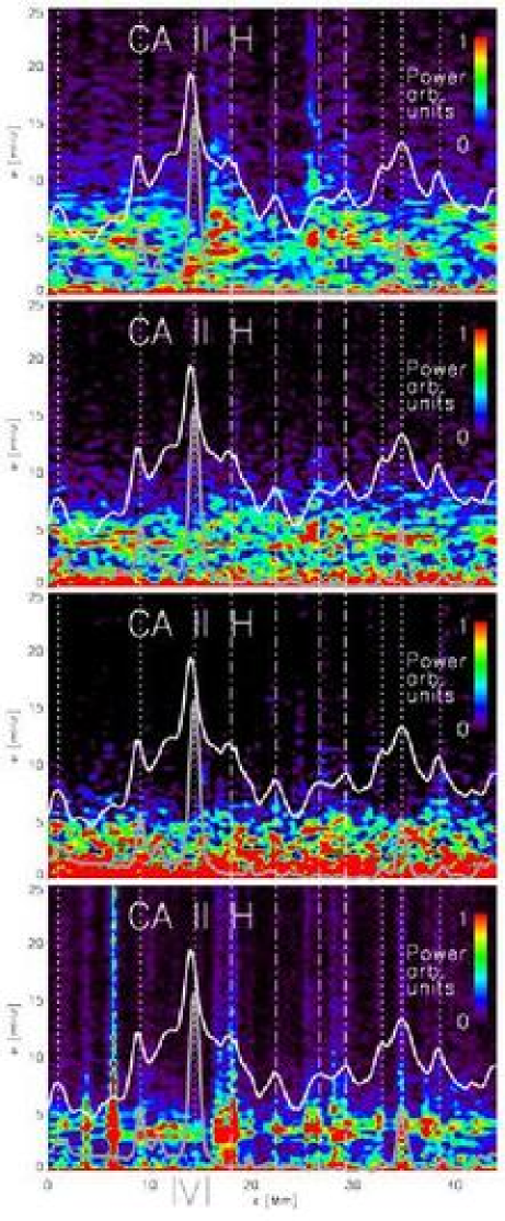
Figure 7: Combination of spatially resolved Fourier power with curves of average H-index (white) and average unsigned Stokes $V$ (grey) along the slit. Top to bottom: power in H_2V, IW,OW, $v_{\rm LOS}$ 630.25 nm. Dotted lines mark enhanced polarization signal, dash-dotted lines enhanced Ca II H emission without strong polarization signal.

k-$\nu$-diagrams

Power spectra of solar oscillations as function of spatial and temporal frequency are a well known tool used in many studies. For the chromospheric Ca II H line few examples using spectroscopy have been published since Cram (1978); in most cases, filtergrams were used (Rutten et al. 2004, or other publications on data from the Dutch Open Telescope). k-$\nu$-diagrams have often been presented for the Ca II K line (Kneer & von Uexküll 1983; Dame et al. 1984; Steffens et al. 1995) or H$\alpha$ (Kneer & von Uexküll 1985). Leenaarts & Wedemeyer-Böhm (2005) show the only k-$\nu$-diagram from a simulation, for a wavelength of 396.74 nm. We will concentrate here mainly on the changes with wavelength in the shape of the k-$\nu$-diagrams. The velocities and intensities up to MW1 show strongest power in the 3-4 mHz range, corresponding to the photospheric 5 min oscillations (Fig. 5). For the inner wing, the frequencies with high power start to increase. For all quantities from the Ca line core, significant power can be found up to frequencies of 10 mHz. The power in the quantities from the line core of calcium is usually spread over a broad frequency range. The power distribution is similar to the one found by Wöger (2006, Figs. 5.11 and 5.12, p. 84ff), who used short-exposed narrow-band Ca II K core images. Only for the broad-band H-index is there a prominent peak near 3 min. This could indicate that, with the increased spatial and spectral resolution and higher S/N ratio in recent observations, more of the fine-structure of the dynamic chromospheric evolution is detected, whereas previous observations using broad-band filtergrams have mainly traced the bright grains with their characteristic 3-min repetition time. Only OW and MW1 do not show reduced power from 1 to 2 mHz, which all other graphs exhibit. The k-$\nu$-diagrams of the line-core velocity oscillations of the Fe I lines (lower left) match more closely to the that of IW1 than that of the outer wing, reflecting the formation of the line cores above the continuum.

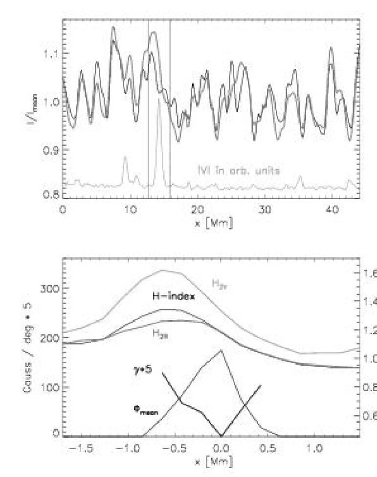
Figure 8: Top: continuum intensity along the slit at 630.4 nm (red channel, black) and in the wing of calcium (blue channel, grey). The Stokes V signal along the slit is overplotted, the strongest concentration is marked by two vertical lines. Bottom: blow-up of the field concentration. Magnetic flux, $\Phi_{\rm mean}$, and field inclination, $\gamma$, are shown at the bottom, intensities in H_2V, H-index, and H_2R at the top.

Average power spectra vs. wavelength

To study the dependence of power on wavelength, $\lambda$, without regard to the spatial extent, we also calculated the k-$\nu$-diagrams for all wavelength points in the Ca spectrum, and averaged over the spatial frequencies. Figure 6 displays the power as function of $\lambda$ for two different normalizations of the Fourier power: using the power at the first non-zero frequency, P($\lambda,\nu$=0.3 mHz), or at 3 mHz, P($\lambda,\nu$=3 mHz). For the first normalization, the power in the Ca line core is strongly reduced compared with the wing; in the second case, the increased power at higher frequencies near the Ca line core shows up prominently. All line cores of photospheric spectral lines also show more medium-frequency power (3-4 mHz$\equiv$ 4-5 min) than their close-by continuum.

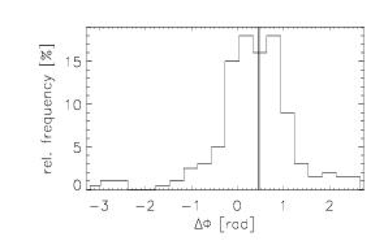
Figure 9: Histogram of phase differences between H_2V and IW1 at $\nu$ = 4.8 mHz. The vertical line marks the center of gravity of the distribution.

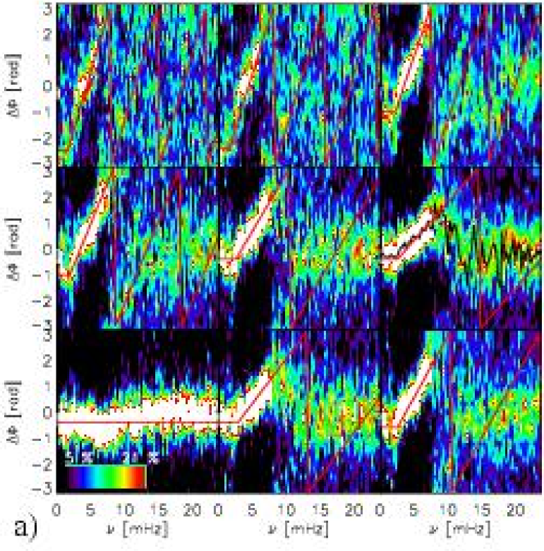
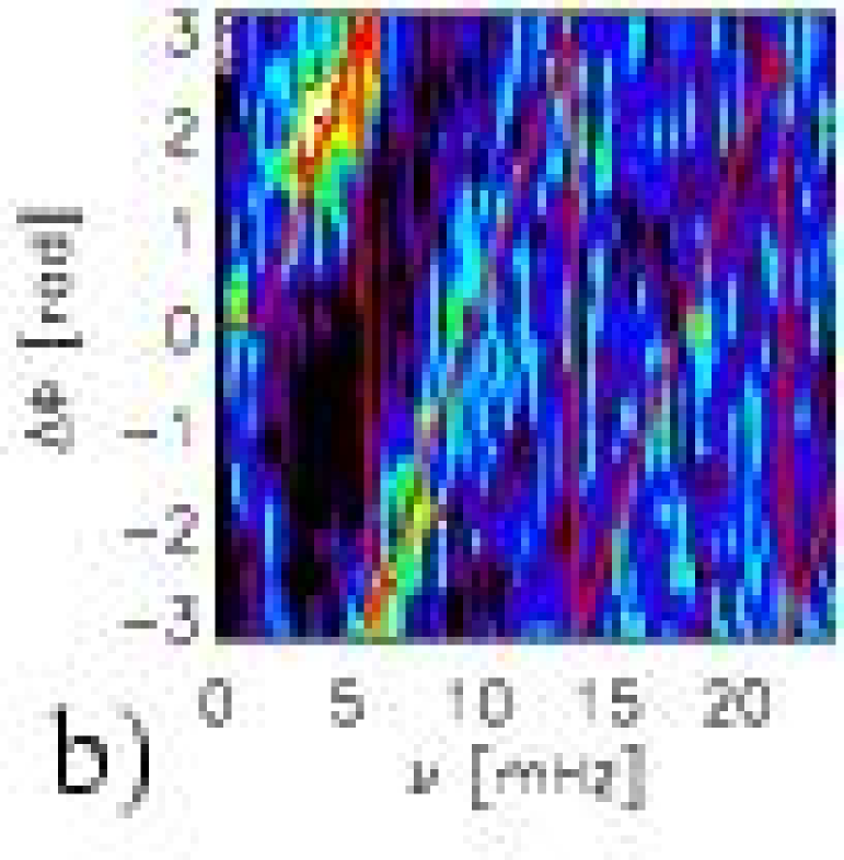
Figure 10: (a) Fourier phase differences between the H_2V emission peak and different wavelengths. For each frequency, the color code (cf. lower left corner) shows the relative occurrence of a given phase shift. Red lines are a manual fit of piecewise defined straight lines to the data. Three parameters were used to construct the curves: a variable offset for $\nu$ = 0 mHz, the minimum frequency of propagating waves ($\sim$ 1-2 mHz), and the slope of the dispersion relation. Top row, left to right: OW, MW1,MW2. Middle row: MW3, IW, IW1. Bottom row: core intensity, RW1, RW2. For IW1, the center of gravity of the phase difference distribution is overplotted in black. (b) Phase difference between H_2V and $v_{\rm LOS}$ 630.15 nm. The phase differences have not been corrected for the 21 sec time difference between the blue and red channel that introduces an additional frequency-dependent phase shift.

                                                                                                               

Spatially resolved power spectra

To investigate the influence of the photospheric fields on the power spectrum, we calculated the power spectrum of each pixel along the slit separately (cf. Lites et al. 1993, their Figs. 4 and 5). Figure 7 shows the spatially resolved power spectrum of the H_2V peak, inner and outer wing, and of the line-of-sight velocity of Fe I at 630.25 nm. For comparison, the unsigned integrated Stokes $V$ signal, $\int|V(\lambda)|d\lambda$ (grey, lower curve) and the H-index (white, upper curve) are overplotted, both averaged over the time series. The enhanced power at high frequencies ($>$ 5 mHz) in the H_2V peak avoids the magnetic fields and is displaced from them by 1 to 3 Mm. This happens at all strong flux patches (dotted lines), but especially at the strongest one at x = 15 Mm. At the location of this field concentration, chromospheric low-frequency power is enhanced. Lites et al. (1993) found the same reduction of high-frequency power and increase of low-frequency power for network fields; enhanced halos of 5 mHz power around network were also found by several authors, for example Krijger et al. (2001). A similar spatial displacement between magnetic fields and high-frequency power can be seen in the inner wing power spectra.

In the outer wing, the power spectrum shows very little spatial dependence at all. The locations of the fields are not significantly different from their surroundings. In contrast, the power in the line-of-sight velocity of the photospheric Fe I line at 630.25 nm shows a strong spatial variation, with several localized sources with high power at all frequencies up to around 6 mHz (x= 6.5,8, 18,35 Mm). Only the last source coincides with strong magnetic fields. We remark that this power spectrum comes from the red channel of POLIS. Enhanced chromospheric intensity is cospatial with either magnetic fields, or increased medium-frequency (2-6 mHz) power. Especially in the power of the photospheric velocity, each local maximum of the H-index not related to magnetic fields is correlated one-to-one with larger than average oscillation power in the photosphere (x=18,22.5,26,28 Mm).

Figure 7 also indicates that the maximum H-index is not cospatial to the field concentration at x=15 Mm. As the curves in Fig. 7 were created from the temporal averages, we decided to use a single scan step for closer investigation of this displacement. To check the alignment of the red and blue channel, the upper panel of Fig. 8 shows the intensity in the (pseudo-)continuum of each channel on scan step 65. The curves clearly show that there is no systematic spatial displacement between the channels. The lower panel shows a blow-up of the strongest field concentration, with the values of field inclination, $\gamma$, and average magnetic flux per pixel, $\Phi_{\rm mean}=B\cdot f\cdot\cos\gamma$, from the inversion. $f$ is the filling fraction of magnetic fields inside the pixel. The largest emission is displaced from the maximum magnetic flux by about 0.65 Mm to the left to a region, where the fields are more inclined ($\sim 25^{\circ}$). The reason for the displacement is not obvious, and the direction seems arbitrary at first. We note however that the flux concentration at x$\sim$10 Mm has the opposite polarity. Field lines connecting these two patches and forming a canopy between them could be the reason that the emission is displaced in that direction.

Phase differences

The phase differences between oscillations at different geometrical heights contain information on the presence and type of waves. Both intensity or velocity oscillations can be related to each other (e.g. Lites & Chipman 1979). As the determination of chromospheric velocities from, e.g., the location of the Ca II H line-core position, is rather unreliable, we only considered intensity oscillations in the following. We have first calculated the phase differences between the oscillations in the H_2V emission peak and the wavelengths bands of Table 1, and later between H_2V and all wavelengths in the blue channel.

We used a method for the creation of phase difference plots similar to that used in previous studies (Lites & Chipman 1979; Kulaczewski 1992; Lites et al. 1993; Leenaarts & Wedemeyer-Böhm 2005). Treating each of the 209 pixels along the slit and each wavelength (band) individually, we derived the phases, and hence, the phase differences as a function of frequency from the Fourier-transform of the intensity variation with time. As there is a 360^∘-ambiguity in the phase differences, i.e. -190${}^{\circ}\equiv+170^{\circ}$, all phase differences have been projected into the range $\pm 180^{\circ}$. We then calculated the histograms of relative occurence of phase differences for each frequency. Figure 9 shows an example for the phase difference between H_2V and IW1 at $\nu$ = 4.8 mHz. The histogram of the phase differences at a given frequency is usually well centered around a single peak. This indicates that there is a preferred phase relation between the different wavelengths, i.e. a (retarded) connection between the oscillations.

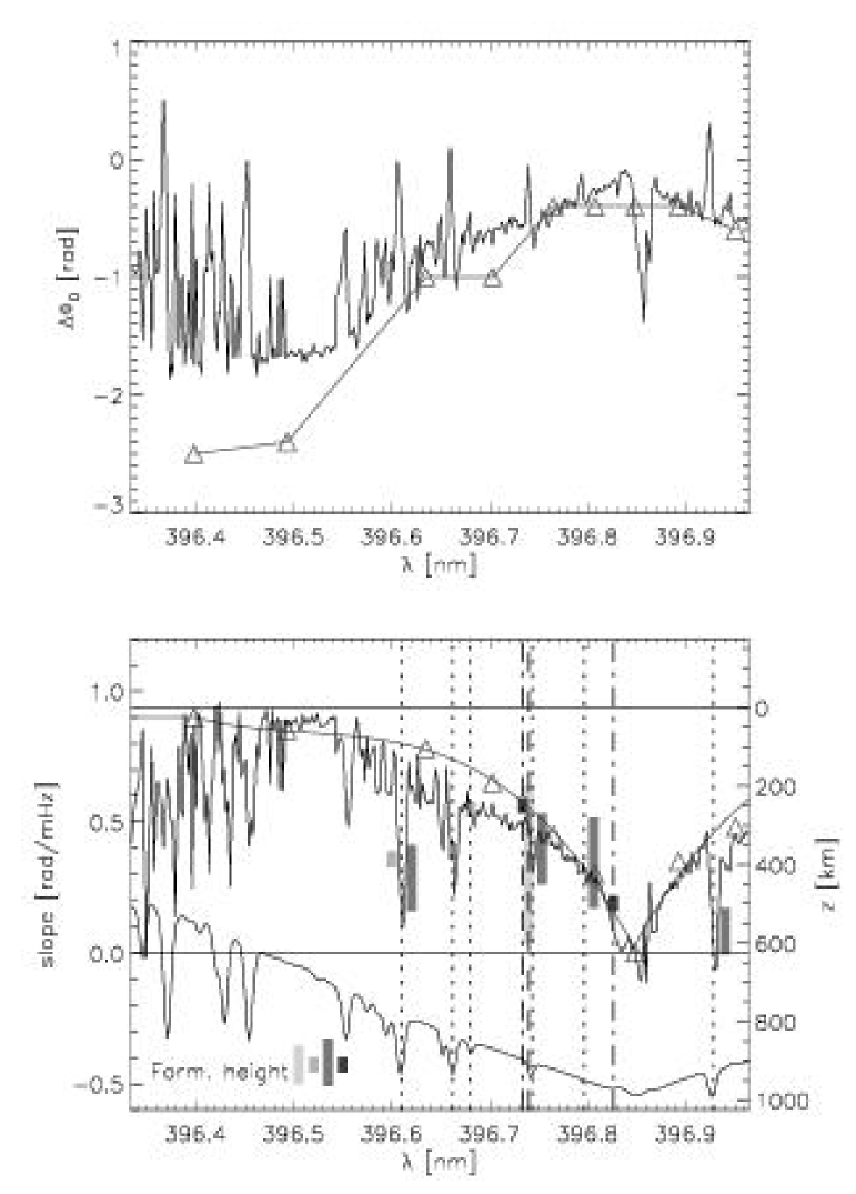
Figure 11: Parameters of straight line fit to phase shifts. Top: phase offset for $\nu<2$ mHz. Bottom: slope of phase shift as function of frequency. Solid black zig-zagging lines: results of automatic fit. $\triangle$: results of manual fit, connected by lines for better visibility. In the bottom panel, the Ca spectrum is overplotted as reference. Dotted vertical lines mark spectral lines. The dashed and dash-dotted vertical lines mark “continuum” wavelengths (396.734 nm, 396.74 nm, 396.826 nm) outside photospheric blends. The grey shaded areas denote formation heights obtained in other studies, plotted according to the scale in km at the right. The horizontal lines mark the zero of the slope and of the geometrical height scale, respectively.

Figure 10 shows the phase differences thus obtained as function of oscillation frequency for wavelength bands going from the outer blue wing of the Ca line through the line core into the red wing. The graph contains several interesting features:

• Reliable phase differences can be determined from 0 up to around 10 mHz.

• Three parameters seem to suffice for the description of the phase difference as a function of frequency: a phase offset for $\nu$ = 0 mHz ($\Delta\Phi_{0}$), a minimum frequency for propagating waves ($\nu_{\rm min}$), and the slope of the dispersion relation ($\delta(\Delta\Phi)/\delta\nu$). Using these three parameters, the observed phase differences can be reproduced by piece-wise straight lines: a constant value of $\Delta\Phi_{0}$ ($\nu<\nu_{\rm min}$), and a straight line with the slope $\delta(\Delta\Phi)/\delta\nu$ ($\nu>\nu_{\rm min}$).

• The phase differences as function of wavelength separation from H_2V, going from wing to the core, then show the following trends: a reduction of $\Delta\Phi_{0}$ from $-\pi$ to 0, a decrease of the slope $\delta(\Delta\Phi)/\delta\nu$, and a small increase of $\nu_{\rm min}$.

• The behavior is symmetrical around the Ca line core, i.e. IW1 (IW) is nearly identical to RW1 (RW2). The phase shift between, e.g., IW1 and RW1 (not shown) was close to zero for all freqencies.

The phase shifts actually show more structure for low frequencies ($<$ 2mHz) in some cases. The behaviour is similar, and can best be seen in the phase shift between H_2V and MW3 (Fig. 10, middle row, at the left). The phase shift starts with zero at zero frequency, decreases with frequency until around 2 mHz, and only then starts to increase with a constant slope. Negtive phases at low frequencies could be indicative of the presence of gravity waves (cf. Krijger et al. 2001).

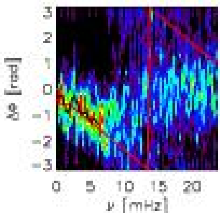
Figure 12: Phase shift between 396.831 nm (H_2V) and 396.853 nm (line core). The straight lines resulted from the automatic fit to the COG values of the phase distributions (black).

As the plot of the phase differences between H_2V and the nine continuum bands showed a “well-behaved” relation, we tried to derive the characteristic values ($\Delta\Phi_{0},\delta(\Delta\Phi)/\delta\nu$) also for all wavelengths $\lambda$ by an automatic method. To this extent, we calculated the phase differences between the intensity oscillations in a single wavelength pixel located in the H_2V emission peak ($\lambda_{0}$ = 396.831 nm) and all other wavelengths in the spectrum of the blue channel in the same way as before. At each frequency, $\nu$, we determined the center of gravity of the phase shift histogram (cf. Fig. 9). To these values of $\Delta\Phi(\nu,\lambda-\lambda_{0})$ (cf. middle row, rightmost panel of Fig. 10 or Fig. 12) we fitted a straight line inside a frequency range from 1.3 mHz to around 5 mHz. This yields values of offset and slope as function of wavelength. From a visual inspection of phase differences and fit result it was seen that the offset value was less well reproduced than the slope. This is due to the fact that a fixed $\nu_{\rm min}$ was used, which affects the derived offset more strongly than the slope. However, the results of the automatic fit were in reasonable agreement with the nine manually derived values, and yield smooth curves for both offset and slope (cf. Fig. 11).

The curve of $\delta(\Delta\Phi)/\delta\nu$ as function of wavelength allows for an interpretation of the smaller slope found for the continuum bands closer to the Ca II line core: the same decrease happens for all wavelengths located in the line cores of spectral lines in the blue or red wing. The reason is that in the most basic formulation of propagating waves in the solar atmosphere the phase difference is given by $\Delta\Phi(\nu)=f(\nu)\cdot\Delta z$, with $\Delta z$ the height difference between two layers, whose phase differences are calculated (e.g. Centeno et al. 2006). $f(\nu)$ should be independent of the wavelengths in the observations related to each other; it reflects the properties of the waves propagating in the solar atmosphere that produce the intensity variations. The change of the slope with $\lambda$ then simply reflects the (non-linear) conversion from wavelength to geometrical height difference, $\Delta z$.

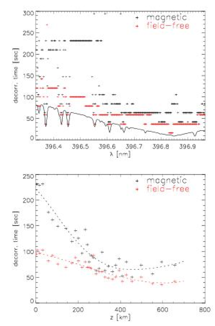
Figure 13: Upper graph: decorrelation time as function of wavelength for magnetic (black) and field-free locations (red, slightly shifted down for better visibility). Lower graph: same as function of geometrical height. The dashed lines are a 3rd order polynomial fit for easier visualization.

The relation between slope and geometrical height can then be used in the opposite direction to determine the formation heights of spectral lines or continuum wavelengths. Deubner (1974) used a similar approach to determine the formation height of some spectral lines. We have added a second axis of geometrical height at the right of the lower panel in Fig. 11, and overplotted some formation height ranges derived from intensity contribution functions for continuum wavelengths (darkest grey, Leenaarts et al. 2006, using the FALC model), from response functions of spectral lines (H. Schleicher, priv. comm., dark grey, published in Beck et al. 2005b), from phase differences (grey, Lites et al. 1993), and from simulations (light grey, Leenaarts & Wedemeyer-Böhm 2005). The formation heights from these other studies are denoted by shaded areas that were drawn slightly displaced in wavelength in some cases for better visibility. We remark that the geometrical scale is determined uniquely by two references height values, z($\lambda_{1}$) and z($\lambda_{2}$), which were simply chosen in the present case. The outermost wing was set to zero height; the formation height of the line at 396.6 nm was used to yield the second value, z($396.6\thinspace{\rm nm})\sim 550$ km. With this caveat, we think the agreement between the formation heights derived from several different methods and the curve of the slope of the phase relation converted to geometrical height to be reasonable, taking into account that the derivation of height from the slope is a rather indirect method. Note that the Ca line core would also be located at only around 700 km according to the height scale. The slope actually turned to values below zero for some wavelengths in the line core (Fig. 12), opposite to the slope in the line wing. This would be required for upwards propagating waves, if the line core forms above the H_2V peak.

3.5 Decorrelation time

To quantify typical time scales, we used the autocorrelation of intensity and the decorrelation time, $\tau$, when the autocorrelation drops below 1/e (e.g., Leenaarts & Wedemeyer-Böhm 2005; Tritschler et al. 2007). We used an automatic method to determine $\tau$ as function of wavelength for field-free and magnetic regions. Figure 13 shows that in the line wing, the decorrelation time inside (outside) fields is around 200 to 250 sec (100 to 150 sec). The decorrelation times get smaller in the chromospheric layers, and are between 21 and 63 sec near the Ca core for both field-free and magnetic regions. Note that due to the temporal sampling of 21 sec this implies a drop of the correlation from 1 to below 1/e in a single time step. Shorter decorrelation times cannot be detected with the cadence of the observations, but cannot be excluded. Directly in the Ca line core (396.86$\pm 0.02$ nm), the decorrelation time reaches again around 100 seconds for the locations with magnetic fields.

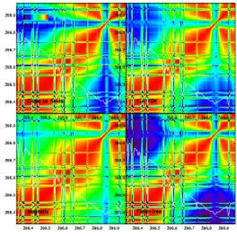
Figure 14: Wavelength correlation matrices. Clockwise, starting top left: area close to magnetic fields, full FOV, field-free region, region with magnetic fields. The scale is $\Delta\lambda$ in nm. All correlations are displayed between -0.3 and 1, a color bar is given in the upper left image.

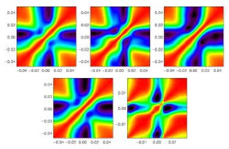
Figure 15: Magnified view of the region around the Ca line core. (Top row, left to right): field-free, close to magnetic fields, magnetic. (Bottom row, left): full FOV, Ca line core. (Bottom row, right): full FOV, Fe I at 396.45 nm.

Using the relation between wavelength and height from Fig. 11, we created a plot of decorrelation time as function of height (Fig. 13). With the caveat that the height scale is not very well determined, the curve may still serve for a fast comparison with simulations, as the decorrelation times of some physcial quantities like temperature, velocity, or opacity in a simulation box at a given height can be derived without spectral synthesis.

3.6 Correlation matrices

Rammacher et al. (2007) suggested investigating the amount of correlation between different wavelengths in chromospheric spectral lines as a fingerprint of the heating process. We thus calculated the correlation matrices for the full wavelength range available in our spectra, and four different spatial areas: the full field of view, field-free regions, regions with photospheric magnetic fields, and an area close to fields, but without photospheric polarization signal (cf. Table 2). The last area has been chosen to be next to the strongest field concentration, where the chromospheric high-frequency power is enhanced (cf. Fig. 7). Figure 14 shows the found 2-D wavelength correlation matrices. The correlation is enhanced over a longer wavelength range, if magnetic fields are present. Without magnetic fields present, anti-correlation is found for wavelengths separated more than around 0.4 nm. The matrix for the full FOV compares well to the one given by Rammacher et al. (2007) for Ca II H (their Fig. 1).

Table 2: Locations of the regions used in Sects. 3.6 and 4 in arcsec along the slit (cf. Fig. 16).

with mag. fields	no magn. fields	close to magn. fields
12-14, 19-22, 48-51	4-11, 24-43	22-25

The correlation matrix is highly structured around the Ca line core and all other spectral lines. This is demonstrated in Figure 15, which shows a magnified view of the Ca line core. The four different spatial areas selected show different correlations, both in the absolute values and the shape of the correlation matrix. Also each spectral line in the Ca line wing produces similar patterns in the correlation matrix (lower right of Fig. 15). If the pattern is produced by the same spectrum of waves in calcium and the other lines, this offers a good opportunity to restrain theoretical heating mechanisms, because the blends in the line wing are better accessible for a detailed modeling than the Ca line core itself, which requires to consider NLTE effects.

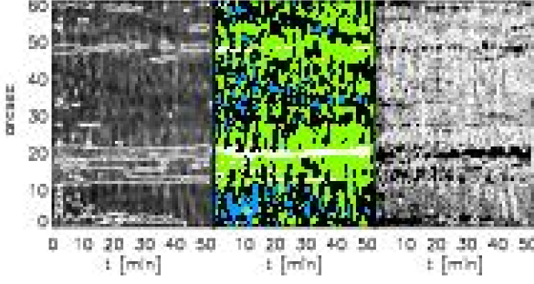
Figure 16: Left: H-index. The upper (lower) diamond at t$\sim$10 min denotes the location of largest (smallest) H-index. Contours outline strong polarization signal. Middle: mask of locations with magnetic fields and strong emission (white), field-free emission (green), and quiet (blue) Ca profiles. Right: integrated Stokes $|V|$ in reversed scaling. Contours outline strong emission.

4 Average Ca profiles: quiet, magnetic, field-free emission

In the previous sections we have concentrated on the global characteristics of the temporal evolution of the Ca profiles. In the following we rather investigate the shape and evolution of individual profiles, in an attempt to identify the process leading to the emission in Ca II H.

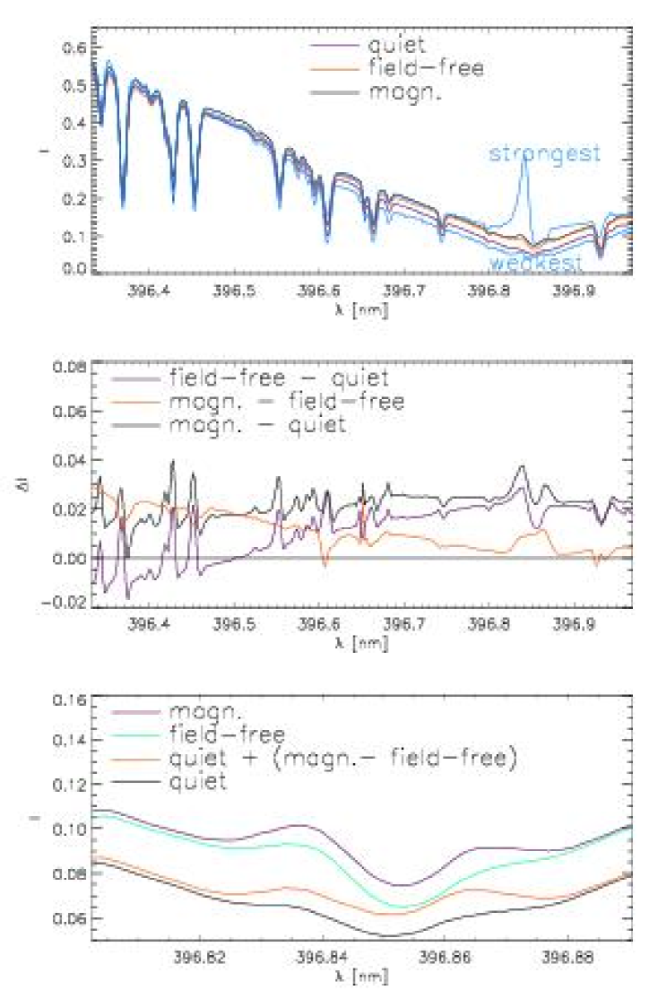
Figure 17: Top: average profiles of locations with magnetic fields, field-free emission, and quiet profiles. Strongest and weakest emission profiles are overplotted. Middle: differences between the average profiles. Bottom: close-up of the line core. The configuration of quiet profile plus the difference of magnetic and field-free profile is no observed profile.

We used the value of the H-index to identify the locations in the field of view, where at a given time some heating process must be (or have been recently) active. We separated all profiles with high emission (H-index $>$ 8 pm) and magnetic fields from those with emission but without fields. As a third sample we selected all locations with strongly reduced H-index ($<$ 7 pm). The resulting mask is shown in Fig. 16. We then averaged the profiles of each sample. The top panel of Fig. 17 shows the resulting average profiles, including the profiles having the largest, respectively, smallest H-index for comparison. To enhance the visibility of the differences between these average profiles, we subtracted them from each other (middle panel). This plot reveals some interesting features. The intensity at locations of photospheric magnetic fields is seen to be higher than the quiet profile at all wavelengths by a roughly constant amount throughout the line wing. In the Ca II H line core, the difference shows two peaks, where the one corresponding to H_2V is more pronounced. In contrast to that, the intensity for locations with field-free emission is higher than the quiet profile only close to the core, whereas the line wing intensity is identical. In the line core, the asymmetry between H_2V and H_2R is increased, the latter is almost invisible. The difference between field-free and magnetic emission shows the opposite slope in the line wing: the intensities close to the core are similar, while in the wing the field-free locations have lower intensity. In the line core, the difference between magnetic and field-free emission only shows a single broad peak, where the H_2R peak is more pronounced.

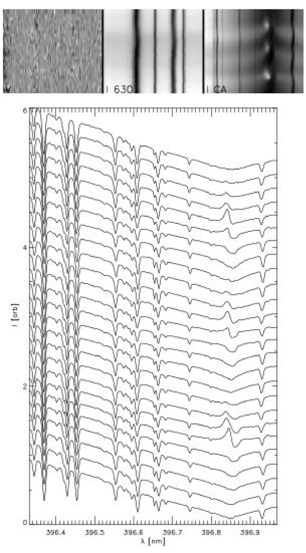
Figure 18: Temporal evolution of spectra at one fixed slit location during 500 sec. Top, left to right: Stokes V, Stokes I 630.4 nm, Ca line core. The individual profiles are displayed at the bottom.

If one assumes that our three samples correspond to a) a non-heated atmosphere (quiet profiles), b) a non-magnetically heated atmosphere (field-free emission), and, finally, c) a magnetically and non-magnetically heated atmosphere (location of fields), one can quantify the characteristic properties of the different heating mechanisms. The non-magnetic heating shows the typical shock signature with an enhanced H_2V peak, while leaving the wing unchanged. The magnetic heating affects the whole spectral range, raises the line wing intensity, and shows a peak symmetric to the line core. This indicates a permanent temperature rise in the upper layers more strongly than the transient emission with the shock signature in the field-free case. The increase in the line wing could be a simple consequence of the shift of the optical depth scale in the presence of the magnetic fields and not related to a heating process at all. It would be interesting to compare the profile resulting from subtracting the field-free emission from the magnetic emission with the difference between synthetic profiles assuming a non-heated chromosphere and a flux concentration embedded in the same atmosphere. Solanki et al. (1991) performed calculations of Ca II K spectra for several flux tube models that could be used for this purpose, if Ca II H spectra were calculated instead.

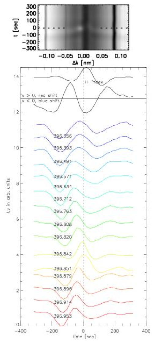
Figure 19: Temporal evolution close to the average shock event at t=0 sec as function of time. Top: average spectra. Bottom: intensity in continuum bands.

5 Shock evolution

The evolution of Ca profiles during the formation and passage of shocks has been extensively studied. The closest reproduction of the patterns observed was achieved by Carlsson & Stein (1997), who employed a photospheric piston that generated upward propagating waves in a 1-D atmosphere. These waves steepened into shocks and led to the appearance of emission in H_2V. The general pattern of the shock signature is also well known (cf. Cram & Dame 1983, or the extensive review of Rutten & Uitenbroek 1991). Figure 18 displays one example of a series of three successive shock waves that are in good agreement with earlier descriptions for the behavior in and close to the Ca line core. With our large wavelength range we can also try to trace down the origin of the shocks leading to the strong emission in H_2V. As can be seen in Fig. 1, both intensity increases and decreases near the Ca line core can be followed down to the outmost wing intensity observed at around 0.5 nm from the core.

To obtain a statistically significant proof of the pattern, we determined the locations of all profiles ($\sim$1000 cases), where the intensity of the H_2V peak exceeded 0.1 of I_c, and averaged them. We did the same with the profiles observed on these locations during the 300 seconds before and after the high emission. This yielded the average evolution of profiles near a shock event (top panel of Fig. 19). From these averaged profiles, we took the intensities in continuum bands as function of time, where the “shock” is at t = 0 sec. The most interesting feature is that the average shock seems to be both preceded and followed by a reduction of intensity, where the reduction is more pronounced before the shock event. The first intensity minimum can be seen to travel smoothly from the wing to the core in around 100 seconds. The maximum following it, culminating in the shock, does not seem to propagate in the same way: in the outer wing ($\lambda<396.571$ nm), the maximum appears later than for, e.g., 396.571 nm. The event classified as the shock also seems on average not to be isolated, but rather to be one of a series of shocks. At around t=-250 sec, an initial intensity increase of H_2V is visible, albeit much weaker than the required intensity of 0.1.

6 Summary & discussion

The chromosphere as a dynamic and transient structure is hard to deal with. Whether it can be described by temporally or spatially averaged quantities or models is a matter of debate (e.g. Kalkofen et al. 1999; Rammacher & Cuntz 2005). Commonly its definition and the proof of its existence are taken to be the temperature rise to values above the photospheric temperature. We use this most basic definition in the following, and use the emission in the Ca II H line as indicator of the temperature rise, and thus the result of some kind of heating process responsible for it. Then two main topics have to be discussed: What are the properties and the evolution of the emission ? To what photospheric structures or events is the emission related ?

Properties of field-free emission

Outside strong photospheric fields, the largest emission in the Ca II H line core appears in the shape of transient brightenings of short temporal (60 sec) and spatial (2-3^′′) extension (“bright grains”). Even if the grains are rather short-lived, the emission takes time to build up to a maximum and relaxes more slowly afterwards (Fig. 18). The grains can repeat some times on the same location with a cadence of around 200 seconds. The chromospheric pattern is markedly different from the evolution of the photospheric granules. The brightenings are mainly due to an increase of intensity of the blue emission peak, H_2V (cf. Figs. 1 or 18). This pattern is well known from the earlier spectroscopic observations of Ca II H or K (e.g. Cram & Dame 1983; Rutten & Uitenbroek 1991, and the references therein) and has been reproduced fairly well by acoustic waves steepening into shocks by Carlsson & Stein (1997).

Temporal coverage of emission

Steffens et al. (1996, S96) estimated that the chromosphere spends only 9 % of the time in a state leading to bright grains. This small amount led Kalkofen et al. (1999) to claim that a reproduction of bright H_2V or K_2V grains does not cover the energy contained in the chromosphere, but rather only a tenth of it. However, we remark that the selection of bright grains in S96 strongly depended on a strict intensity threshold. To quantify the amount of time spent in (strong) emission without imposing a threshold, we took the profiles of the quiet Sun region in the middle of the observed FOV (cf. Table 2, 2nd row), and classified them according to increasing H-index. The average profiles in seven bins in the H-index and their spatio-temporal area fractions are displayed in Fig. 20. For an H-index below around 7.5 pm, the average profiles show only weak emission features. If the H-index exceeds 7.5 pm, a pronounced asymmetry of H_2V and H_2R is seen. Profiles with a strongly enhanced H_2V peak cover around 6% of the area, in agreement with S96. If however the area fractions of all profiles with emission signatures (H-index $>$7.5 pm) are added up, the ratio of profiles in emission to those without is 60:40. Taking the full FOV, the area fraction of profiles with an H-index above 7.5 pm is 64 %. Another estimate can be made from Fig. 18: a shock event affects usually three to four profiles, i.e. it leads to emission for 60 to 80 seconds afterwards. If the next shock happens 180 seconds after the first one, the fraction of time spent in emission is around 70/180$\sim$40 %. This definition of the emission from the appearance of any H_2V peak then suggests in all estimates that the chromosphere, or more precisely, the core of the Ca II H line spends around half of the time in emission instead of 10 %. If this emission can by modeled by a static temperature rise, or reflects a temperature rise at all, is another question.

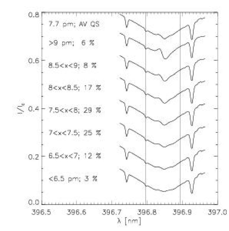
Figure 20: Average profiles corresponding to different levels of the H-index, with their relative occurence in a field-free region. The two vertical lines denote the emulated 1-Å filter that yields the H-index.

Emission in relation to magnetic fields

On locations with detected photospheric fields, a quasi-permanent increase of intensity in both emission peaks is present, in addition to similar repetitive bright grains as happen outside fields. Near to, but still outside strong photospheric magnetic fields, the emission is generally increased (cf. Figs. 4 or 16). Interestingly, the maximum H-index observed in the time series is located outside of magnetic fields, which could fit with the suggestion of Kalkofen (1996) that collisions between flux concentrations and granules are responsible for the creation of bright grains. We note however that in our case it would be the interaction of a strong uni-polar network element with granulation instead of the weaker mixed-polarity fields suggested by Kalkofen (1996).

The areas with least chromospheric emission in our time series are located furthest away ($>10^{\prime\prime}$) from any magnetic fields, in the middle of the observed field of view. The spatial distribution of emission in our 1-D slit observations would comply very well with a cut through the FOV observed by Vecchio et al. (2007, V07), if the slit would be placed across one of the field concentrations visible in their Fig. 2. The halo of enhanced emission close to the fields found in the present paper would correspond to one high-emission fibril seen in the Ca II 854.2 nm line by V07. These fibrils are interpreted to reflect the chromospheric magnetic field topology by V07, and end after around $10^{\prime\prime}$ in low-emission dark regions.

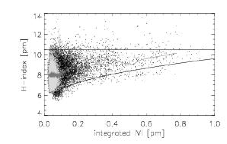
Figure 21: Scatter plot of integrated unsigned Stokes $V$ signal vs the H-index. Black dots: full FOV. Light grey dots: quiet area without network. The grey line gives the average value of H-index as function of $V$. Black lines outline upper and lower limits of the H-index.

Like Lites et al. (1999), we do not see an one-to-one correlation of emission in calcium and photospheric fields or Stokes $V$ signal as claimed by Sivaraman et al. (2000), in none of the Figs. 1, 4, or 16. Lites et al. (1999) employed data very similar to ours, spectro-polarimetry in 630 nm and spectroscopy in Ca II H. There are several occurrences of H_2V brightenings on locations without any polarization signal above our detection limit of 0.15 % of the continuum intensity. The relation in the other direction is however rather tight: if photospheric fields are present, the emission is enhanced and often also affects the H_2R peak as well (Figs. 1 and 4). To quantify the visual impression, we use the scatter plot of integrated unsigned Stokes $V$ signal vs the H-index (Fig. 21). The scatter plot of the full FOV shows the usual behavior (e.g. Skumanich et al. 1975; Schrijver 1987; Schrijver et al. 1989; Rezaei et al. 2007), a general increase of chromospheric emission with polarization signal, i.e., with total magnetic flux. To substantiate the claim that emission can occur without fields, we overplotted the values of the quiet region in the middle of the FOV (cf.Table 2, 2nd row) separately in light grey. It can be clearly seen that the emission in this part of the FOV covers the same range in the H-index as the full FOV, from 6 to around 11 pm, but shows only weak polarization signals. We emphasize also again the conclusion of Rezaei et al. (2007) that the presence of magnetic flux influences the minimum H-index, but that the maximum emission value seems to be independent of the magnetic flux. This gives another indirect argument that photospheric fields increase the chromospheric emission, but do not actually deliver the main contribution to it.

For the strongest concentration of magnetic flux in the field of view observed, a stable long-lasting ($>1$ hr) network element, we find a displacement of 1^′′ between magnetic flux and highest emission, and less pronounced photospheric power. The displacement is only in one direction along the slit, which we ascribe to the field topology in the FOV. The strongest field concentration could be connected to one of opposite polarity nearby in the direction of the displacement.

Properties of intensity oscillations

The chromospheric intensity oscillations show power at all frequencies from 0 to about 10 mHz. We do not find a pronounced peak of power at 3 minutes, but a broad distribution over several frequencies. However, to address the question of heating, the average power spectrum alone is of less interest than the power spectrum of locations with strong chromospheric emission. Comparing the spatially resolved chromospheric intensity with chromospheric and photospheric oscillation power, or with the locations of photospheric fields, it can be seen that strong emission in the chromosphere is always related to one of two things (or both): magnetic fields, or high power in the photospheric velocity oscillations. These photospheric oscillations are due to isolated small-scale power sources in the frequency range up to the acoustic cutoff frequency of around 5 mHz (cf. Fig. 7, lowermost panel). This agrees with the finding of Kamio & Kurokawa (2006) that the large-scale photospheric 3 mHz oscillations are less important for the generation of H_2V bright grains than localized 5 mHz oscillations (see also Hoekzema et al. 2002). The result would also be in agreement with both an impulsive excitation of waves, or a stochastic generation by the (random) superposition of large-scale wave patterns, which again would interfere positively only on some locations.

The analysis of the phase differences between the oscillations of the H_2V peak and the intensities at other wavelengths gives evidence that the acting agent between photosphere and chromosphere are propagating waves with frequencies above 2 mHz. Below 2 mHz, constant phase shifts are found that however depend on the wavelength difference to the H_2V peak. For frequencies above 2 mHz, the phase differences to H_2V allow to determine the slope of the phase difference as function of oscillation frequency, $\delta(\Delta\Phi)/\delta\nu$, for all wavelengths in the observed spectral range around the Ca line core (-0.5 nm,+0.1 nm). This quantity can be used to derive an estimate of the formation height, as the phase difference is in the basic approximation directly proportional to a height difference.

Wöger et al. (2006) used a threshold of 150 sec in the decorrelation time to identify network areas in their narrow-band Ca II K filtergram observations. For their remaining internetwork sample, they obtained a typical time scale of around 50 sec. Figure 13 then suggests that the separation between network and internetwork by a decorrelation time of 150 sec should only work properly, when information from the lower chromosphere is included in the observations. Above 400 km height, the locations of magnetic fields show decorrelation times around 100 sec, whereas on the field-free locations we also find around 50 sec. We suggest using a lower threshold of around 75 sec, as at least the results agree that field-free locations should show decorrelation times below that. Figure 13 also implies that the pattern of inverse granulation, presumably originating at heights between 200 km and 600 km (e.g. Leenaarts & Wedemeyer-Böhm 2005), has a smaller decorrelation time than the photospheric granulation itself. The inverse granulation pattern also does not show up prominently in the intensity maps at different wavelengths (Fig. 4).

Evidences of propagating waves

That the waves responsible for the chromospheric emission are traveling from the photosphere upwards, is shown by an analysis of the temporal evolution of profiles at fixed locations. The brightest grains with strong H_2V emission can all be traced back to intensity variations in the outermost line wing observed. The pattern travels from the wing (396.35 nm) towards the line core (396.85 nm) in around 50-100 seconds, corresponding to phase speeds between 7 and 14 kms^-1 with the height scale derived from the phase differences. Interestingly, both intensity decreases and increases can be seen traveling through the spectrum, where the brightest grains are on average preceded and followed by an intensity decrease (cf. Fig. 19). Cadavid et al. (2003) found a similar phenomenon, where however darkenings of G-band were either preceding or following a brightening in their rather broad-band (3Å) Ca II K filtergrams. In our case, the darkening preceding a shock could appear, because most bright grains are part of a train of successive brightenings with darkenings in between.

Selection sensitivity

We caution that our results may be biased by selection effects. Our spatio-temporal field of view covers 60${}^{\prime\prime}\times$ 1 hr, with a specific configuration of strong photospheric fields inside of it. Several quantities (power spectra, average profiles, wavelength correlation matrices) were found to be sensitive to the locations chosen in their derivation. Even if we tried to select the locations by the commonly used criteria of network fields and internetwork areas devoid of strong fields, we cannot exclude the possibility that we have observed an “atypical” network field, because a single field concentration more or less dominated the signal for the “magnetic” locations. Analysis of more data will be needed to exclude such effects. Fortunately, several other time series were taken with POLIS in 2006 in observation campaigns previous to the one used here, albeit with a worse temporal sampling.

7 Conclusions

We have analyzed a time series of intensity spectra in the chromospheric Ca II H line and Stokes vector polarimetry in the two Fe I lines at 630 nm. We derived the statistical properties of the emission pattern visible in the H_2V and H_2R peaks near the Ca line core. We find that the emission is mainly due to two sources: isolated small-scale sources of strong photospheric oscillations, or magnetic fields. The presence of strong photospheric fields adds only some quasi-static emission to a pattern of transient brightenings as in field-free locations. The emission is generally enhanced near the photospheric fields, and smallest when furthest away from the field. The main driver of the chromospheric emission of Ca II H are seen to be acoustic waves, propagating upwards from the photosphere and steepening into shocks, and not the magnetic fields. We estimate that the temporal fraction of Ca II H profiles in emission is around 50%, whereas bright H_2V grains happen around 6% of the time only. The emission seems to be always related to shock events, either in their increasing or decreasing phase.

We analyzed a spectral range from around 396.33 nm to 396.97 nm on the signature of the chromospheric heating process. We suggest that these wavelengths in the line wing of Ca II H, and the spectral lines located there, may be more helpful for the study of the chromosphere than thought of before (see also the review of Rutten 2007). The propagating waves leave clear traces in the phase differences between core and wing, the wavelength correlation matrices, or simply the wing intensity. Even an inversion of spectra assuming LTE is able to follow a (shock) wave through the wing (cf. Appendix B).

We find that the chromospheric heating as seen in the emission near the Ca II H line core is dominated by propagating acoustic waves coming from the photosphere, in agreement with the “piston model” of Carlsson & Stein (1997). Magnetic fields influence the energy deposit by waves in and near them, which could be related to the “magnetic portal” effect (Jefferies et al. 2006), but they seem to be of minor importance and do not supply the energy of the chromospheric heating (cf. Lites et al. 1999; Rezaei et al. 2007). If the emission in Ca II H represents the chromospheric temperature increase, and thus, the heating process, its origin are acoustic waves.

The still transient emission in Ca II H – even if we estimate around 50% temporal filling fraction – seems to be in contradiction to the permanent emission required to explain the SUMER observations of Carlsson et al. (1997, CS97) in far-UV spectral lines. We suggest a difference in formation height for an explanation of the discrepancy as sketched in Fig. 22. We see a changed behavior of the emission in and close to photospheric magnetic fields, in comparison to locations far from the magnetic fields ($\sim$10^′′) . This implies that in the formation height of Ca II H the magnetic fields have not yet expanded enough to fill the whole volume of the chromosphere. If the emission lines of CS97 originate from higher layers, which are magnetic everywhere and can be affected by magneto-hydrodynamic waves inside the fields, the part-time emission at only some locations of the lower chromospheric layers ($\equiv$ acoustic heating) can be reconciled with a permanent emission in the whole volume above it ($\equiv$ magneto-acoustic heating): the magnetic field lines connect the whole volume to photospheric oscillation sources, whereas in the lower field-free chromosphere the waves can affect only a small volume on their way. The question if and where the magnetic fields form a closed canopy would then be crucial for investigations of the chromospheric heating process.

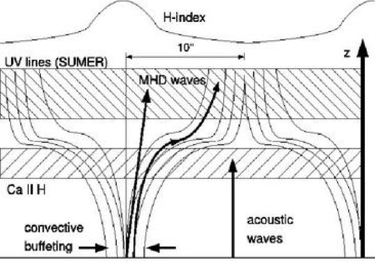
Figure 22: Sketch of the formation height of Ca II H and the emission lines of Carlsson et al. (1997) in relation to a possible magnetic field topology.

Appendix A Differential refraction effects for POLIS

As discussed in Reardon (2006), the differential refraction in the Earths’ atmosphere leads to a wavelength dependent spatial displacement. The relative displacement between two wavelengths, ($\lambda_{1},\lambda_{2}$), can be calculated directly from the refraction index, $n(\lambda_{1},\lambda_{2}$). The refractive index of air has been derived by various groups (e.g. Filippenko 1982; Stone 1996; Livengood et al. 1999, and references therein). For all following calculations, we have used the equations given by Filippenko (1982), which yield the refractive index, $n_{\rm final}(\lambda,P,T,H)$, as function of temperature, humidity, pressure, and wavelength. The displacement in arcseconds between two wavelengths $(\lambda_{1},\lambda_{2})$ is then given by:

$$\Delta R(\lambda_{1},\lambda_{2})=\kappa\cdot\tan\,Z\cdot\left[n_{\rm final}(\lambda_{1})-n_{\rm final}(\lambda_{2})\right],$$ (1)

where $Z$ is the zenith distance of the object under examination, and $\kappa$ is the conversion coefficient from radian to arcsecsonds, $\kappa=180/\pi\cdot 3600=206265$.

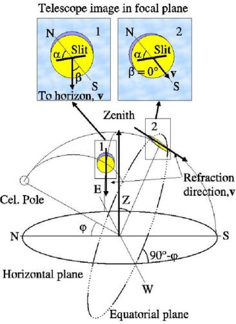
Figure 23: Effects of differential refraction in the Earth’s atmosphere: $\phi$ is the geographical latitude, $Z$ the zenith distance of the Sun. The differential refraction acts along the line connecting Sun center and horizon, v, causing a vertical displacement of the solar image for different wavelengths. To derive the corresponding displacement along and perpendicular to the slit in the focal plane, the angles $\beta$, between CNS and v, and $\alpha$, between CNS and the slit, have to be known. The image in the focal plane of the telescope has been depicted for two cases: 1 Somewhen after sunrise: CNS and v are not parallel, $\beta\neq 0$. 2 Meridian passage of the Sun: CNS and v are parallel, $\beta=0^{\circ}$. $\alpha$ is constant for a coelostat system.

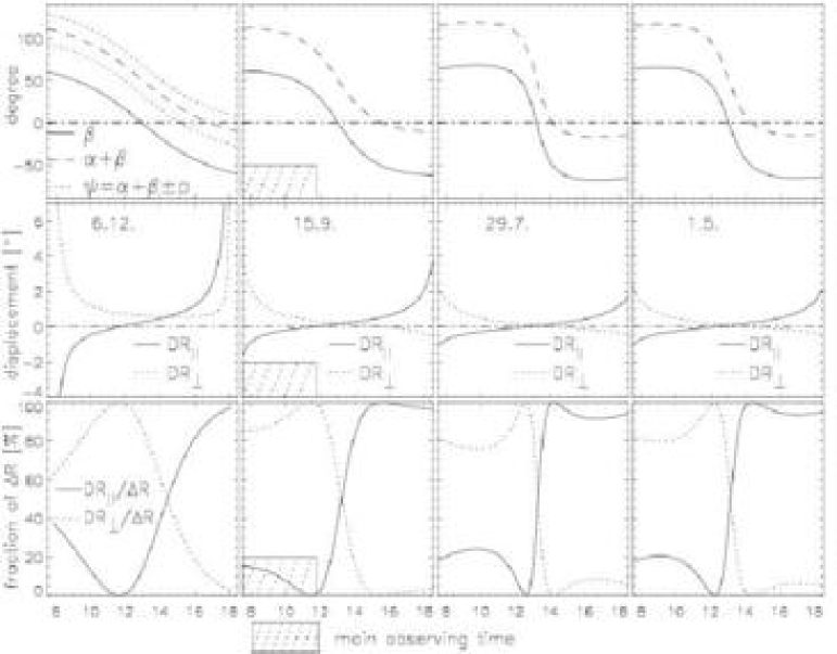
Figure 24: Angles used in the calculation, and the final displacements parallel and perpendicular to the slit for the two POLIS channels on four dates. Top row: The angle $\psi$ determines the relative fraction of $\Delta R_{\perp}$ and $\Delta R_{\parallel}$. $\beta$ denotes the orientation of celestial N-S to the local vertical; it has to pass zero at noon. The fixed slit orientation adds a constant amount $\alpha$ to $\psi$. The additional image rotation by the coelostat, $p$, can either in- or decrease $\psi$, depending on the sign of $\gamma$. Middle row: The displacements due to the differential refraction along the slit, $\rm DR_{\parallel}$ (solid), and perpendicular to the slit, $\rm DR_{\perp}$ (dotted). Bottom row The fraction of $\Delta R_{\parallel}$ and $\Delta R_{\perp}$ of the total displacement $\Delta R$. Left to right: Parameters for 6.12., with $\gamma=\pm 90^{\circ}$, and for 15.9., 29.7. and 1.5., with $\gamma=0^{\circ}$. During the main observing time from 8-12 UT the displacement is mainly perpendicular to the slit.

However, for a dual-channel slit-spectrograph instrument with a fixed slit like POLIS the main concern is not the absolute displacement, but the fraction perpendicular to the slit. Thus, the direction of the displacement between images in different wavelengths, $I(\lambda)$, in the focal plane has to be determined as well. The calculation of the direction of the displacement in the focal plane can be separated into three steps, a) the projection of the dispersion axis of the $I(\lambda)$ into the focal plane, b) effects due to the telescope, and c) effects due to the orientation of the slit.

A.1 Projection of the dispersion axis into the focal plane

If the position of the Sun in equatorial plane coordinates, declination, $\delta_{\odot}$, and hour angle, $t_{\odot}$ is taken from an ephemeris table, the zenith distance, $Z$, in horizontal plane coordinates can then be derived by:

$$Z_{\odot}={\rm arccos}(\sin\phi\cdot\sin\delta_{\odot}+\cos\phi\cdot\cos\delta_{\odot}\cdot\cos t_{\odot})\;,$$ (2)

where $\phi$ denotes the geographical latitude. With $Z$ the absolute displacement can be calculated from Eq.(1).

The celestial North-South (CNS) axis is defined by the tangent to the great circle through Sun center and the celestial north pole at $\delta=\delta_{\odot}$. The dispersion axis, v, is analogously given by the tangent to the great circle through Sun center and the zenith point. The parallactic angle, $\beta$, then denotes the angle between the CNS axis and the dispersion axis. From the spherical triangle pole-Sun-zenith it can be derived that

$$\beta={\rm arctan}\left(\frac{\sin t_{\odot}}{\cos\delta_{\odot}\cdot\tan\phi-\sin\delta_{\odot}\cdot\cos t_{\odot}}\right)\;.$$ (3)

$\beta$ incorporates the time-dependent part of the direction of the spatial displacement, which is due to the daily solar revolution on the sky.

A.2 Image rotation due to the telescope

A coelostat telescope system may introduce an additional image rotation in the focal plane. A displacement of the first coelostat mirror by the angle $\gamma$ from the terrestrial N-S axis leads to a constant image rotation, $p$, which is given by:

$$p=-{\rm arcsin}\left(\frac{\cos\phi\cdot\sin\gamma}{\cos\delta_{\odot}}\right)+\gamma\;.$$ (4)

A.3 Instrument orientation in the focal plane

Finally, for a slit-spectrograph the orientation of the slit relative to CNS has to be considered. This will be denoted by the angle $\alpha$ between the slit and the CNS axis as defined above. For a coelostat system, $\alpha$ and $p$ are constant during the day and depend only on the telescope and instrument geometry. The angle, $\psi$, between the slit and the dispersion axis is then given by the addition of all contributions:

$$\psi=\beta+(p+\alpha)\;,$$ (5)

where the parentheses indicate the contribution due to telescope and instrument orientation. The displacements perpendicular, $\Delta R_{\perp}$, and parallel to the slit, $\Delta R_{\parallel}$, are then given by:

$$\begin{pmatrix}\Delta R_{\perp}\cr\Delta R_{\parallel}\cr\end{pmatrix}=\begin{pmatrix}\sin\psi\cr\cos\psi\end{pmatrix}\cdot\Delta R(\lambda_{1},\lambda_{2}),$$ (6)

with $\Delta R(\lambda_{1},\lambda_{2})$ from Eq. (1).

Figure 24 shows the resulting displacements for the two POLIS channels at 396 nm and 630 nm on four dates. For observations on 24th of July, at around UT 8:00, a displacement perpendicular to the slit of around 2^′′ can be read off.

Appendix B LTE inversion examples

Figure 25: Histogram of field strength in the inversion.

Two inversions were performed, one in the full field-of-view (FOV) using only the spectra of the red channel, the second in a restricted area including the Ca intensity spectra in the fit as well. The FOV contained only few locations with magnetic fields, which mainly were stable network elements persisting throughout the 1-h time series. The distribution of field strengths in Fig. 25 thus shows mainly fields around 1.3 kG. Note that due to the fixed slit position the same flux concentration contributes multiple (up to 150 !) times.

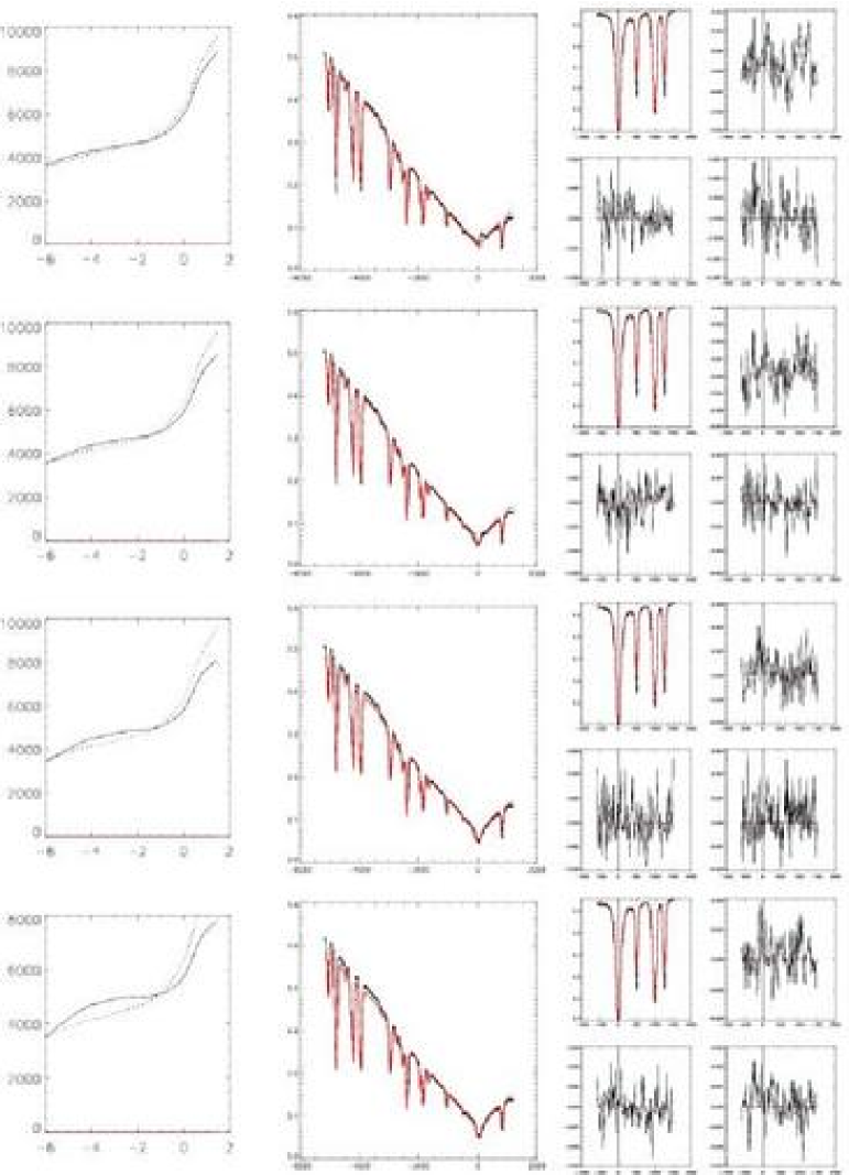
Figure 26: Examples of the LTE inversion. Left: temperature stratification. Middle: Ca spectra (black), best-fit profiles (red). Right: same for 630 nm, clockwise: IQUV.

Figures 26 and 27 show examples of the LTE inversion results with the SIR code, where the complete Ca II H intensity spectrum and Stokes $IQUV$ of the 630 nm channel were used in the fit. The inversion scheme employed a straylight contamination with the average quiet Sun profile, and a field-free inversion component. The straylight contribution was generally always larger than 80 %. As the amount of chromospheric heating contained in the straylight profile is non-zero (two reversals in Ca II H intensity profile, Fig. 20), the results of the field-free inversion component will tend to underestimate the temperature increase.

The profiles were taken from the same spatial location and show the temporal evolution during 168 seconds. The NLTE effects in the Ca II H line core can of course not be recovered. However, the inversion still yields a temperature increase in the upper atmospheric layers that travels upwards in optical depth with time. The amplitude and properties of this temperature increase are actually not governed by the line core, but the line wing intensities close to the Ca II H core, where LTE maybe still applies. Note that on this display scale the actually still existing mismatch between fit and observations in the 630 nm channel can not be seen at all. To summarize, it seems feasible very well to reproduce the photospheric spectra and the Ca line wing at the same time with a “reasonable” temperature stratification including a chromospheric temperature rise.

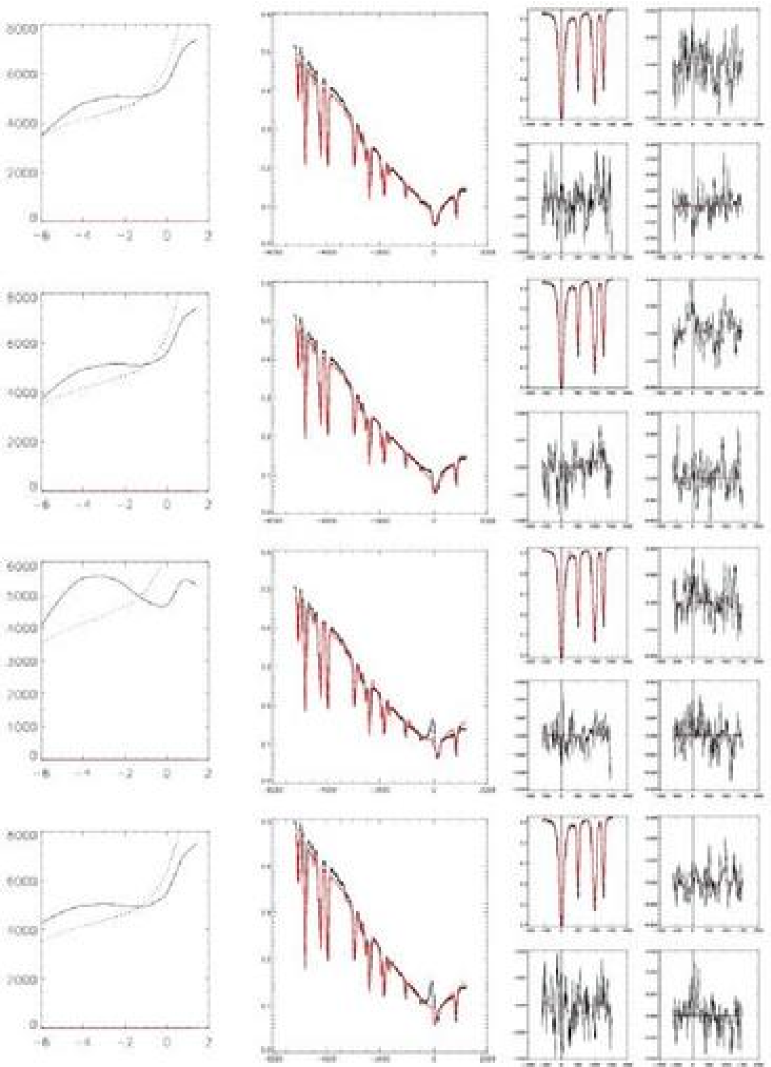
Figure 27: Same as previous Fig.