Sunyaev-Zeldovich profiles for clusters and groups of galaxies

Abstract

The Sunyaev-Zeldovich (SZ) effect gives a measure of the thermal energy and electron pressure in groups and clusters of galaxies. In the near future SZ surveys will map hundreds of systems, shedding light on the pressure distribution in the systems. The thermal energy is related to the total mass of a system of galaxies, but it is only a projection that is observed through the SZ effect. A model for the 3D distribution of pressure is needed to link the SZ signal to the total mass of the system. In this work we construct an empirical model for the 2D and 3D SZ profile, and compare it to a set of realistic high resolution SPH simulations of galaxy clusters and groups, and to a stacked SZ profile for massive clusters derived from WMAP data. Furthermore, we combine observed temperature profiles with dark matter potentials to yield an additional constraint, under the assumption of hydrostatic equilibrium. We find a very tight correlation between the characteristic scale in the model, the integrated SZ signal, and the total mass in the systems with a scatter of only 4%. The model only contains two free parameters, making it readily applicable even to low resolution SZ observations of galaxy clusters. A fitting routine for the model that can be applied to observed or simulated data can be found at http://www.phys.au.dk/~haugboel/software.shtml.

1. Introduction

When Cosmic Microwave Background (CMB) photons pass through galaxy clusters, they Compton up-scatter on hot electrons, making a small increment (decrement) above (below) the peak of the CMB primary spectrum. The size of this distortion in the CMB spectrum, the Sunyaev-Zeldovich (SZ) effect (Sunyaev & Zeldovich, 1972), is proportional to the electron pressure integrated along the line-of-sight. Besides being an important probe of the physics of the intracluster medium, the SZ effect is a promising tool in cosmology: The signal produced by a cluster is practically redshift independent and can be observed to high redshifts. The Planck surveyor satellite (Tauber, 2000) will produce a cluster catalogue with up to $\sim$10.000 (sufficiently massive) clusters out to $z\sim 1$ (Schäfer et al., 2006). By combining SZ and X-ray observations of relaxed clusters the Hubble constant $H_{0}$ can be derived, limits can be put on $\Omega_{m}$, and the gas mass fraction in clusters can be measured (Bonamente et al., 2005; LaRoque et al., 2006). The SZ effect was first detected in three nearby clusters more than two decades ago by Birkinshaw et al. (1984), but the last five years, due to advances in sub millimetre receiver technology, routine measurements have been done for $\mathcal{O}(100)$ clusters using facilities such as the OVRO and BIMA telescopes. Right now a large number of telescopes have started observing the SZ signal or are under construction (e.g. ACBAR, CARMA, SUZIE III, SPT, APEX etc.), and in the near future ALMA will gradually become online enabling unprecedented resolution and sensitivity for making detailed observations of individual clusters. Current SZ surveys of galaxy clusters (see e.g. Bonamente et al., 2006, for a set of current observations) have observed the unresolved integrated SZ signal from clusters, but with CARMA, ALMA and the SPT also the SZ signal as a function of radius from the cluster centre will be measured. Afshordi et al. (2007) has used the 3rd year WMAP data to extract SZ images from 193 clusters. Stacking them they have obtained an averaged SZ profile for clusters with $T_{X}>3$keV.

Spatially resolved SZ images probe, in a way complementary to X-ray observations, the distribution of thermal energy in clusters which in turn is closely linked to the total cluster mass. Furthermore, since the SZ effect essentially depends on the electron pressure, the physics going into understanding it is simpler and more robust, than is the case for the X-ray emission.

In this paper we use realistic high resolution N-body/SPH simulations of galaxy clusters and groups together with observed temperature profiles of nearby groups and clusters to predict the radial SZ profile of different types of systems of galaxies, and compare our results to the averaged profile of Afshordi et al. (2007). We introduce a universal fitting formula, with only two free parameters, that can be employed in future observations. Furthermore, we show that fitting this profile enables a precise estimate of the total mass in the system. In the next section we describe the computer experiments, that are used to construct the synthetic SZ profiles. In section 3 we discuss the simulated data and present our results, and in section 4 we discuss and provide our conclusions.

2. Computer experiments

We use 24 galaxy group and galaxy cluster simulations to study the SZ effect for systems of virial temperatures of about 1 to 6 keV. The models include 12 groups of approximately the same mass ($M_{vir}=0.8-1.1\times 10^{14}M_{\odot}$), 11 identical clusters with $M_{vir}=2.7\times 10^{14}M_{\odot}$ (“Virgo” clusters), but simulated with different gas physics, and a single large cluster of $M_{vir}=12\times 10^{14}M_{\odot}$ (a “Coma” cluster). The models are re-simulated from a low resolution cosmological dark matter simulation, where the halos are identified with a halo finder. The particles are traced back in time to a initial redshift $z_{initial}$, and the virial volume is repopulated with both gas and dark matter at a high resolution. The code includes radiative cooling, star formation, supernova feedback, chemical evolution and back reaction from a redshift dependent UV field. The different models are summarised in Table 1. For a detailed description of the different gas physics going into the code in general, and the “Virgo” cluster simulations in particular we refer to Romeo et al. (2006). The groups were all selected at random, the only criterion being their virial mass, and therefore they comprise a cosmological fair sample of groups with $M_{vir}=0.8-1.1\times 10^{14}M_{\odot}$.

The different masses of the clusters allow us to probe the mass dependence of the SZ profile, while the “Virgo” models are used to investigate how robust our predictions are for the SZ profile with respect to assumptions on the underlying physics. The groups, being a statistically unbiased sample, give limits on cosmic variance for the given virial mass ($10^{14}M_{\odot}$).

We have divided the groups into three different classes according to their morphology and evolutionary history: Groups with merging activity (186,231,239,262), fossil groups (189,228,236,244) and normal groups (190,233,247,276). A group is considered fossil if the difference in apparent R-band magnitude of the first and second brightest galaxy is greater than two (Jones et al., 2000), and a group is merging if it by visual inspection has significant merging activity in the core, or if the rms scatter in 3D radial shells of the temperature, pressure and density, is comparable to the average value in the shell.

Name	$T_{X}[\textrm{keV}]\,\,$	$\,\,T_{mg}[\textrm{keV}]\,\,$	$\,\,M_{180}[10^{14}M_{\odot}]$	Comments
Groups	Re-simulated groups with $z_{initial}=39$
186	0.99	1.08	$0.92$	Merging group
189	1.07	1.09	$0.91$	Cool-Core, Fossil group
190	1.21	1.22	$0.99$	Normal group
228	1.07	1.10	$0.85$	Cool-Core, Fossil group
231	0.99	1.08	$0.84$	Merging group
233	1.03	1.09	$0.82$	Normal group
236	1.00	0.99	$0.73$	Fossil group
239	0.91	1.11	$0.81$	Merging group
244	1.13	1.08	$0.80$	Fossil group
247	1.01	1.15	$0.90$	Normal group
262	0.97	1.03	$0.88$	Merging group
276	1.02	1.07	$0.82$	Cool-Core group
Clusters	Re-simulated clusters with $z_{initial}=19$
AY-SW	2.13	2.07	$2.32$	Arimoto-Yoshii IMF
AY-SW-8	2.18	2.10	$2.36$	8 times resolution
AY-Vol39	2.18	2.18	$2.36$	$z_{initial}=39$
AY-SWx2	2.18	2.04	$2.40$	2 times SNII feedback
AY-SWx4	2.17	2.09	$2.38$	4 times SNII feedback
AY-PH0.75	2.23	2.10	$2.41$	preh. $0.75\textrm{keV}/$part @ z=3
AY-PH1.5	2.27	2.14	$2.37$	preh. $1.5\textrm{keV}/$part @ z=3
AY-PH50	2.19	2.07	$2.41$	preh. $50\textrm{keV}\cdot\textrm{cm}^{2}$part @ z=3
AY-COND	2.26	2.08	$2.43$	Thermal conduction
Sal-SW	2.24	2.10	$2.42$	Salpeter IMF
Sal-WFB	2.27	2.23	$2.41$	Weak feedback
Coma	5.57	5.27	$10.4$	Relaxed massive cluster

Table 1Characteristics of simulated clusters

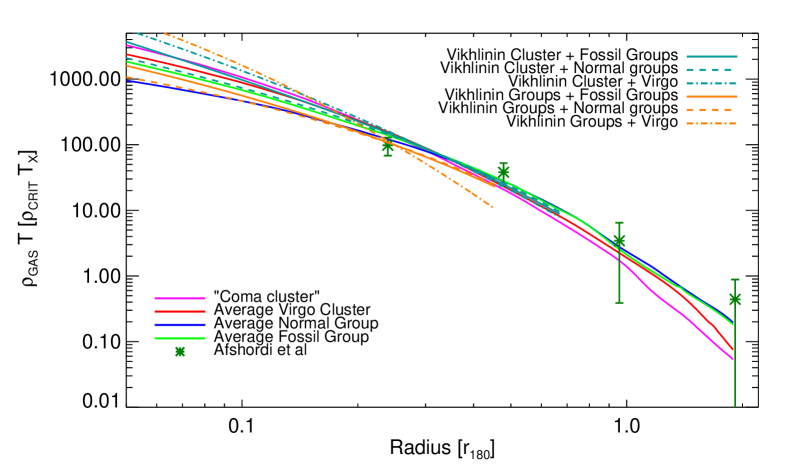
Figure 1.— Spherically averaged 3D SZ profiles computed from the simulations, the stacked profile of Afshordi et al. (2007), and derived 3D profiles from observed X-ray temperatures combined with average gravitational potentials. The profiles are normalised to the critical density $\rho_{CRIT}$, and the typical temperature of the system, $T_{X}$, defined as the average projected spectral-like temperature in the interval $0.1\,r_{200}<r<0.4\,\,r_{200}$. To reduce the visual scatter only average profiles from the simulations are shown.

3. Analysis

The SZ profiles of the simulated systems can only be used as templates for an universal fitting formula, if the profiles are in accordance with observations. In 1 are shown the spherically averaged SZ profiles compared to the only currently published SZ profile (Afshordi et al. (2007)), obtained using data from the WMAP satellite. The observed points may indicate a slightly more bended profile than the simulations, but within the 1-$\sigma$ error bars there is fairly good agreement. From the simulations there is a clear trend towards steeper profiles, for more massive and relaxed clusters and groups reflecting differences in the underlying DM potentials (see 2). This should be recalled when constructing an average observational profile, because the average profile may not represent a true (“universal”) physical profile, but rather a smeared average of the real profiles.

3.1. The inner part of the Sunyaev-Zeldovich profile

The central core of the SZ profile ($r<0.25\,r_{180}$ cannot be probed by WMAP, due to its limited resolution of at most $0.12^{\circ}$. To extend the dynamic range of the observations we combine gravitational potentials from the simulations with observed average X-ray temperature profiles. Under the assumption of hydrostatic equilibrium in the core of the systems, we can then predict the inner part of the SZ profile.

The Compton $y$-parameter, which determines the overall temperature decrement in the CMB radiation due to the SZ effect, is proportional to the integrated pressure $P$ of the electrons along the line of sight

$$y=\int y(l)dl=\int\frac{\sigma_{T}P(l)}{m_{e}c^{2}}dl=\int\sigma_{T}n_{e}\frac{k_{B}T_{e}}{m_{e}c^{2}}dl\,.$$ (1)

Assuming hydrostatic equilibrium and spherical symmetry

$$\frac{dP}{dr}=-\rho_{g}\frac{GM(r)}{r^{2}}$$ (2)

we can use the proportionality of $P$, and the Compton $y$-parameter in a volume element, $y(l(r))$, to obtain

$$\ln\frac{y(r)}{y(r_{0})}=\ln\frac{P(r)}{P(r_{0})}=-\mu_{g}m_{p}\int^{r}_{r_{0}}\frac{GM(r^{\prime})}{k_{b}Tr^{\prime 2}}dr^{\prime}$$ (3)

We have constructed three different averaged gravitational potentials based on the normal groups, the fossil groups and the “Virgo” clusters. For the temperature profiles we use observed clusters by Vikhlinin et al. (2005), and make one average profile constructed from the galaxy groups with virial temperatures less than 2.5 keV, and one constructed from the massive clusters in the sample with virial temperatures between 3.5 and 8.5 keV. The dark matter distribution, derived from the simulations, is quite robust against the specific gas physics involved in the simulation. This is demonstrated in 2, where it is seen that all the “Virgo” models, in spite of the different gas physics, have essentially the same gravitational potentials from $0.02\,r_{180}$ and outwards. However, there are systematic differences between different types of systems with the same mass. Fossil groups are more relaxed compared to normal groups, and their mass distribution is similar to relaxed clusters, like the “Virgo” and “Coma” models from $0.02\,r_{180}$ and outwards (see 2). Therefore the above reconstruction procedure gives a good idea of future resolved SZ observations of the cores of clusters of galaxies, and our six resolved profiles are a fair sample of what can be expected.

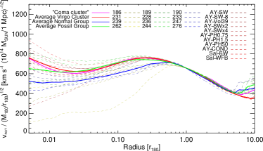
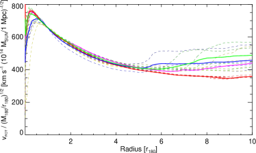
Figure 2.— Dark matter potentials measured as the equivalent rotational speed, both for specific groups and clusters, and for the average “Virgo” cluster, normal and fossil group. The curves are normalised with the virial mass.

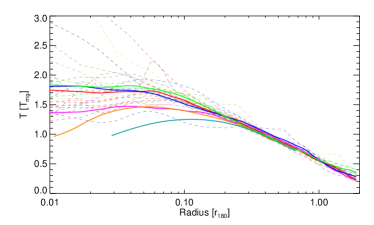
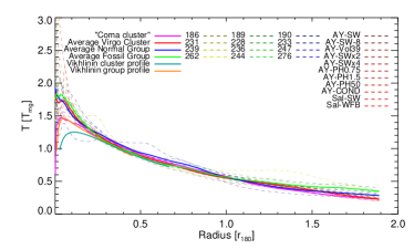
Figure 3.— Mass-weigthed 3D temperature profiles for the simulated systems compared to observed an average group profile (1.6 keV$<T_{X}<$ 2.6 keV), and an average cluster profile (3.5 keV $<T_{X}<$ 8.5 keV).

3.2. Temperature profiles

From 1 it is clear, that albeit the SZ profiles constructed from the observed temperature profiles and the dark matter density profiles are in approximate agreement with the profiles extracted from the simulations, they have a tendency to be more peaked at the centre. This can be traced to differences in the observed and simulated temperature profiles (see e.g. Eq. 3), and to the typical masses of the observed systems. The different temperature profiles are normalised with a global temperature $T_{X}$. To enable direct comparison to the observed temperature profiles by Vikhlinin et al. (2005) we compute $T_{X}$ as the average projected spectral-like temperature (Rasia et al., 2005) in the interval $0.1\,r_{200}<r<0.4\,\,r_{200}$. All profiles converge to the same universal curve for $r>0.2\,r_{180}$, but in the inner part of the systems there are differences (see 3). The simulated systems have all flat profiles at the core, which are in good qualitative agreement with observations of clusters of similar virial mass, but the average observed profiles have lower normalised temperatures towards the centre, with more or less the same offset between the “Coma” cluster and the observed cluster profile (constructed from clusters with 3.5 keV $<T_{X}<$ 8.5 keV), and between the average simulated and observed group temperature profiles (the latter constructed from groups with $T_{X}<2.5$ keV Vikhlinin et al. (2006)). The offset compared to observations and relatively flat temperature profiles are well known problems for simulations invoking radiative cooling and feedback processes (e.g. Borgani et al., 2004; Pratt et al., 2006), but it is further accentuated by an offset in mass between the observed and simulated groups and the observed clusters, and the simulated “Virgo” clusters.

3.3. A universal SZ profile

As can be seen in 1 all the SZ profiles have nearly the same form, but the overall normalisation, tension and slope of the different profiles depends on the mass, and the specific cluster. To construct a simple model we have tried to fit a variety of combinations of beta profiles and exponential profiles for the density combined with a polytropic or isothermal equation of state, but it does not yield a satisfactory fit. The correct temperature to use, when constructing a SZ profile, is the mass weighted, and it does not necessarily agree with the temperature inferred from X-ray observations (Bonaldi et al. (2007); Afshordi (2007)), which may explain why the above combination works well for X-ray observations, while not so for our sample of SZ profiles.

To circumvent this problem we are using a novel universal profile that directly fit the data, without assuming anything about the underlying temperature and density distributions, while using as few parameters as possible. The main morphological differences are in the slope/tension and in the normalisation of each profile, and it is indeed possible to construct a model, that with only two free parameters, a normalisation, and a characteristic scale can fit the full set of simulations and observations in detail.

The profiles extracted from the simulated data do not per se contain any errors, but a measure of the natural scatter in a profile $y(r)$ at a given radial distance, is the variance $\sigma(r)$ of $y(\bf r)$ inside the radial bin at $r$. We have used this variance estimate to construct a goodness of fit parameter $\chi^{2}$ for each projected 2D and spherically averaged 3D profile $y_{2D}(r)$, $y_{3D}(r)$ given by

$$\chi^{2}_{2D,3D}=\frac{1}{r_{max}-r_{min}}\int_{r_{min}}^{r_{max}}\frac{\left(y_{2D,3D}(r)-y^{m}_{2D,3D}(r,\bf p)\right)^{2}}{\sigma_{2D,3D}^{2}(r)}dr\,,$$ (4)

where $y^{m}_{2D,3D}(r,\bf p)$ is the model with parameters $\bf p$. The internal scatter in relaxed systems is much smaller, giving stronger constraints than from merging systems. This is sensible, since the observational scatter among relaxed clusters is smaller too.

We have found that using a triple exponential model gives an excellent fit to the data:

$$y^{m}_{3D}(r)= Y_{m}\left[f_{1}\exp(-r/r_{0})+f_{2}\exp(-r/(\alpha_{2}r_{0}))\right.$$

$$\quad\left.+f_{3}\exp(-r/(\alpha_{3}r_{0}))\right]\,,$$ (5)

where $f_{1}+f_{2}=1$. While this model at first sight might appear complicated, it has two attractive features: (i) The 2D profile can be derived in a closed form from the 3D profile. (ii) Most of the parameters can be fixed to global values, leaving only two free parameters for fitting all systems considered in this paper. With only two parameters in the model it can readily be applied to future observations, even if they only map the SZ profile with a few observational points. By integrating along one of the axes we find the 2D profile to be

$$y^{m}_{2D}(r)= 2\,Y_{m}\left[f_{1}K_{1}(r/r_{0})+f_{2}K_{1}(r/(\alpha_{2}r_{0}))\right.$$

$$\qquad\left.+f_{3}K_{1}(r/(\alpha_{3}r_{0}))\right]r\,,$$ (6)

where $K_{n}(x)$ is the modified Bessel function of the second kind. Minimising $\chi^{2}_{2D}$ simultaneously for all models over the range $0.01\,r_{180}<r<1.9\,r_{180}$, while varying $f_{i}$ and $\alpha_{i}$ as global parameters, and $Y_{m}$, $r_{0}$ for each model, treating the $x-$, $y-$, and $z-$projections as different clusters, we find the global best fit parameters to be

$$f_{1}=0.043$$ (7)

$$f_{2}=1-f_{1}=0.957$$ (8)

$$f_{3}=5.9$$ (9)

$$\alpha_{2}=0.36$$ (10)

$$\alpha_{3}=0.115\,,$$ (11)

In 4 we see how these yield very reasonable $\chi^{2}$ for all projections, and the 3D profiles. The only systems that have a $\chi^{2}$ significantly larger than one are either merging, or characterised by a very smooth profile with almost no variation in the radial bin, and hence a very small $\sigma(r)$ (see e.g. 5).

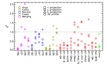
Figure 4.— The goodness of fit parameter for the different models. It is mostly one group with extreme merging activity, and the very smooth models for the “Virgo” cluster, with thermal conduction or entropy floor, that the model have problems with fitting.

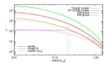
Figure 5.— Examples of the model fits to the SZ profiles with error bars. Two of the profiles represent some of the poorest fits, and illustrate why they are poor fits: The 239 group has a poor fit because of the merging activity, the flatness inside– and spike at $0.2\,r_{180}$ is due to the two central galaxies, separated by approximately $0.4\,r_{180}$, while the AY-Cond “Virgo” cluster has a poor fit because the thermal conductivity in the model gives a very smooth cluster with small error bars. The two others are a representative group and cluster, both with well fitted profiles.

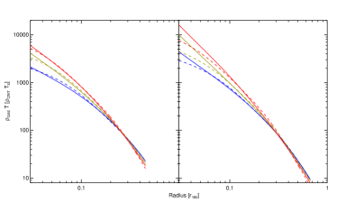
Figure 6.— The fitted profiles for the observed average profile for massive clusters (top), and for the constructed profiles assuming hydrostatic equilibrium, and using average dark matter profiles from the simulations, and observed temperature profiles for groups (bottom left) and massive clusters (bottom right). The red, yellow, and blue curves are for the average “virgo” cluster, fossil group, and normal group DM potentials.

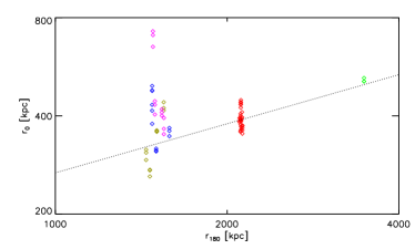
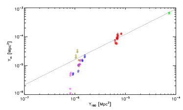
Figure 7.— The slope $r_{0}$ (top) and the overall normalisation (bottom) in the model. The fossil groups act as an extension of the clusters, with the same scaling relation.

The two free parameters, the overall scale $r_{0}$, and the overall normalisation $Y_{m}$ scale with $r_{180}$ and with $Y_{180}$, the integrated SZ effect inside $r_{180}$, respectively, but there is a large scatter between different clusters, where the tightest relation is found for the fossil groups, that act as an extension of the clusters with almost the same scaling relation. They are related as

$$Y_{m}= 15\,\left(\frac{Y_{180}}{10^{-6}\,\textrm{Mpc}^{2}}\right)^{0.9}10^{-6}\,\textrm{Mpc}^{2}$$ (12)

$$r_{0}= 280\left(\frac{r_{180}}{1000\textrm{kpc}}\right)^{1/2}\!\!\textrm{kpc}$$ (13)

To push the boundaries of our fitting formula for other systems we have also applied it to the Afshordi et al. (2007) data, and the profiles for the centre of the systems, derived from observed temperature profiles (see 6). The average SZ profile is described well by the formula , while there are problems with fitting the core ($r<0.05\,r_{180}$) of the cluster set of central profiles (the lower right panel in 6). Even though some of these combinations (e.g. a normal group DM potential combined with a massive cluster temperature profile) are extreme, the lack of agreement may be because in the central parts of the observed systems there are significant non-thermal contributions to the pressure balance from e.g. an AGN (Roychowdhury et al., 2005) or from cosmic rays (Pfrommer et al., 2007), and hence the assumption of hydrostatic equilibrium does not apply. Or it may be that the simulated systems do not include an adequate description of the physical processes in the centre of the systems. Nonetheless, the contribution of the central $0.05\,r_{180}$ to the total SZ signal is approximately 5%, and the parameters are not much affected even if we cannot reconstruct the innermost part of the profiles with perfection.

3.4. Estimating the total mass in a system

The SZ profile of the systems seems to be universally well described by only two parameters, except for possibly in the central parts of the clusters. It measures the distribution of thermal energy in the system, and is therefore related to the gravitational potential, if we assume the system is relaxed. Using assumptions about hydrostatic equilibrium and using a phenomenological approach several “Fundamental plane” relations have been constructed (e.g. Afshordi, 2007; Verde et al., 2002). The main ingredients for the Fundamental plane has been the integrated SZ effect and a characteristic scale in the system, for example $R_{SZ,2}$, the radius enclosing half of the integrated signal. This has given a relation between the integrated SZ effect, a characteristic scale, and the total mass with a rough scatter of 14% (Afshordi, 2007). With our fit to the profiles we get a very precise measurement of this characteristic scale, that take into account the different bending of the profiles. Fitting the total mass as a function of $Y_{180}$ and $r_{0}$ we find (see 8)

$$M_{180}=1.02\,\times 10^{14}M_{\odot}\,\left(\frac{Y_{180}}{10^{-6}Mpc^{2}}\right)^{0.57}\!\!\left(\frac{r_{0}}{1000kpc}\right)^{0.27}\!\!\!\!\!\!\!\!\!\!\!$$ (14)

with only a 4% scatter. In Afshordi (2007) a phenomenological model is used to construct a set of, essentially, one dimensional models for the clusters. It includes normal or tophat distributed controlling parameters, with broadening in agreement with observed clusters. To check if the smaller scatter we see for Eq. 14 is due to more similarity in the simulated systems, we have tried to use the fundamental plane of Afshordi (2007), on the simulated systems. We find good agreement with a 15% scatter for our data (see 8).

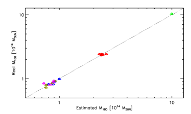
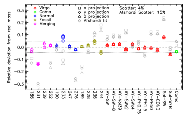
Figure 8.— The estimated mass (from Eq. 14) against the real mass of the systems (top), and the relative error (bottom). The dotted line indicate the rms scatter. For comparison we have included the error on the estimated masses using the method of Afshordi (2007) as light grey symbols.

The first resolved SZ profiles will be obtained for nearby massive clusters. To make a crude test for how our fitting formula works on real data, we have made a set of mock observations taking as a starting point the most massive cluster in our sample, the “Coma” cluster. We use five logaritmically spaced rings at a distance of $[0.09,0.18,0.35,0.7,1.4]\,r_{180}$. The resolution of the first generation of SZ instruments is limited, and therefore we have chosen not to include observational points at smaller radii. To get a good measure of the scatter we generated $10^{4}$ mock observations, with normal distributed logarithmic error bars of 0.22 dex on the total in each ring $y_{i}$, giving an relative error of $\sim 50\%$ on $y_{i}$ itself. For simplicity we have disregarded any correlation there may exist between the different radial bins, and artificially have fixed the relative errors to a uniform level. The five rings are then fitted (see 9) using Eq. (6) giving $r_{0}$. The integrated SZ effect $Y_{180}$ for each mock observation is found by integrating the fitted profile. Inserting $r_{0}$ and $Y_{180}$ derived from each mock observation into Eq. (14) we find a reconstructed mass of $M_{180}=10.0\pm 1.4\times 10^{14}M_{\odot}$, or an $14\%$ error on the reconstructed mass. There is a $4\%$ systematic offset compared to the real mass of $10.4\times 10^{14}M_{\odot}$. With five rings the error on the total signal is $\sim\sqrt{5}\,\,50\%=22\%$. The mass goes roughly as $Y_{180}^{0.57}$, and we would expect roughly a $13\%$ error on the mass, in agreement with what is found.

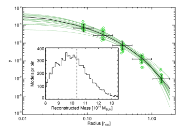
Figure 9.— A set of mock observations based on the “Coma” cluster. The green diamonds, artificially scattered in the radial direction for visibility, are the mock observations, while the thin green lines are corresponding fitted profiles. The black line is the “Coma” SZ profile, with 1-$\sigma$ errors and the width of each ring overplotted. In the inset histogram is shown the distribution of the reconstructed masses. The dotted line is the real mass, which is slightly offset compared to the average reconstructed mass.

4. Discussion

In this paper we have constructed a simple empirical model for the radial profile of the Sunyaev Zeldovich effect in groups and clusters of galaxies. The model has been motivated by, and validated against a mixture of simulations and observations, and is characterised by only two parameters: The overall normalisation, and a typical length scale related to the slope of the profile. It gives a very good fit to the simulated systems, and there is a tight relation between the parameters and the total mass of the system. Furthermore, the results are robust to the detailed gas physics employed in the simulations. This can be seen by considering the subset of the systems, the “Virgo” clusters, that are started from the same initial conditions, but simulated with different implementations of the gas physics (see Table 1). Because of the different gas physics there is an appreciable scatter in $Y_{180}$, but still the mass ($M_{180}$) of the clusters is well reconstructed (see 8).

The simulations are in good agreement with an observed average profile extracted from WMAP data for the outer part of the SZ profiles $0.2\,r_{180}<r<2\,r_{180}$. Currently there are no published high resolution observations of the core SZ profile, but we can get an indirect measure by using temperature profiles extracted from clusters observed in X-rays together with dark matter potentials from the simulations. Reconstructing the SZ profile, under the assumption of hydrostatic equillibrium, we see that these “core profiles” are relative peaked, compared to the simulations. This is traced to differences in the temperature profile of the simulated systems, compared to what is observed using X-rays. We have to await future observations of the resolved cluster cores, to determine to what extent this cusp in the central part is real, or a result of the hypothesis of hydrostatic equilibrium, which is known to be violated in the centre of clusters of galaxies, where non-thermal processes such as AGN heating (Roychowdhury et al., 2005), and cosmic rays (Pfrommer et al., 2007) can play an important role for the pressure balance.

We stress that the model we have presented here is readily applicable to future observations. This will give a good proxy for the mass of the observed system. It will also help in reconstructing the full SZ profile from observations with low spatial resolution, to be used in conjunction with X-ray observations in the study of cluster dynamics. A fitting routine written in IDL for the profile that can be applied to observed or simulated data can be found at
http://www.phys.au.dk/~haugboel/software.shtml.

References

- Afshordi et al. (2007) Afshordi, N., Lin, Y.-T., Nagai, D., & Sanderson, A. J. R. 2007, MNRAS, 378, 293
- Afshordi (2007) Afshordi, N. 2007, ArXiv e-prints, 704, arXiv:0704.2416
- Birkinshaw et al. (1984) Birkinshaw, M., Gull, S. F., & Hardebeck, H. 1984, Nature, 309, 34
- Bock et al. (2006) Bock, D. C.-J., et al. 2006, Proc. SPIE, 6267 (see also http://www.mmarray.org/)
- Bonaldi et al. (2007) Bonaldi, A., Tormen, G., Dolag, K., & Moscardini, L. 2007, MNRAS, 478
- Bonamente et al. (2005) Bonamente, M., Joy, M., LaRoque, S., Carlstrom, J., Reese, E., & Dawson, K. 2005, Bulletin of the American Astronomical Society, 37, 1430
- Bonamente et al. (2006) Bonamente, M., Joy, M. K., LaRoque, S. J., Carlstrom, J. E., Reese, E. D., & Dawson, K. S. 2006, ApJ, 647, 25
- Borgani et al. (2004) Borgani, S., et al. 2004, MNRAS, 348, 1078
- De Grandi & Molendi (2002) De Grandi, S., & Molendi, S. 2002, ApJ, 567, 163
- Jones et al. (2000) Jones, L. R., Ponman, T. J., & Forbes, D. A. 2000, MNRAS, 312, 139
- LaRoque et al. (2006) LaRoque, S. J., Bonamente, M., Carlstrom, J. E., Joy, M. K., Nagai, D., Reese, E. D., & Dawson, K. S. 2006, ApJ, 652, 917
- Pfrommer et al. (2007) Pfrommer, C., Enßlin, T. A., Springel, V., Jubelgas, M., & Dolag, K. 2007, MNRAS, 430
- Pratt et al. (2006) Pratt, G. W., Boehringer, H., Croston, J. H., Arnaud, M., Borgani, S., Finoguenov, A., & Temple, R. F. 2006, ArXiv Astrophysics e-prints, arXiv:astro-ph/0609480
- Rasia et al. (2005) Rasia, E., Mazzotta, P., Borgani, S., Moscardini, L., Dolag, K., Tormen, G., Diaferio, A., & Murante, G. 2005, ApJ, 618, L1
- Roychowdhury et al. (2005) Roychowdhury, S., Ruszkowski, M., & Nath, B. B. 2005, ApJ, 634, 90
- Romeo et al. (2006) Romeo, A. D., Sommer-Larsen, J., Portinari, L., & Antonuccio-Delogu, V. 2006, MNRAS, 371, 548
- Schäfer et al. (2006) Schäfer, B. M., Pfrommer, C., Bartelmann, M., Springel, V., & Hernquist, L. 2006, MNRAS, 370, 1309
- Sommer-Larsen et al. (2005) Sommer-Larsen, J., Romeo, A. D., & Portinari, L. 2005, MNRAS, 357, 478
- Sunyaev & Zeldovich (1972) Sunyaev, R. A., & Zeldovich, Y. B. 1972, Comments on Astrophysics and Space Physics, 4, 173
- Tauber (2000) Tauber, J. A. 2000, IAU Symposium, 201 (see also http://www.rssd.esa.int/index.php?project=Planck)
- Verde et al. (2002) Verde, L., Haiman, Z., & Spergel, D. N. 2002, ApJ, 581, 5
- Vikhlinin et al. (2005) Vikhlinin, A., Markevitch, M., Murray, S. S., Jones, C., Forman, W., & Van Speybroeck, L. 2005, ApJ, 628, 655
- Vikhlinin et al. (2006) Vikhlinin, A., Kravtsov, A., Forman, W., Jones, C., Markevitch, M., Murray, S. S., & Van Speybroeck, L. 2006, ApJ, 640, 691