CERN-PH-TH/2007-252

ROM2F/2007/20

DESY 07-220

FTUAM-07-20

IFT-UAM-CSIC-07-64

MKPH-T-07-25

December 2007

Non-perturbative renormalisation of ${\Delta F=2}$
four-fermion operators in two-flavour QCD

P. Dimopoulos^a, G. Herdoiza^b, F. Palombi^c,

M. Papinutto^c, C. Pena^d, A. Vladikas^a and H. Wittig^e

^a INFN, Sezione di Roma II

and Dipartimento di Fisica, Università di Roma “Tor Vergata”

Via della Ricerca Scientifica 1, I-00133 Rome, Italy

^b DESY, Platanenallee 6, D-15738 Zeuthen, Germany

^c CERN, Physics Department, TH Division, CH-1211 Geneva, Switzerland

^d Departamento de Física Teórica C-XI and

Instituto de Física Teórica UAM/CSIC C-XVI

Universidad Autónoma de Madrid, Cantoblanco E-28049 Madrid, Spain

^e Johannes Gutenberg Universität, Institut für Kernphysik

Johann Joachim Becher-Weg 45, D-55099 Mainz, Germany

 Abstract Using Schrödinger Functional methods, we compute the non-perturbative renormalisation and renormalisation group running of several four-fermion operators, in the framework of lattice simulations with two dynamical Wilson quarks. Two classes of operators have been targeted: (i) those with left-left current structure and four propagating quark fields; (ii) all operators containing two static quarks. In both cases, only the parity-odd contributions have been considered, being the ones that renormalise multiplicatively. Our results, once combined with future simulations of the corresponding lattice hadronic matrix elements, may be used for the computation of phenomenological quantities of interest, such as $B_{K}$ and $B_{B}$ (the latter also in the static limit).  

1 Introduction

Hadronic matrix elements of four-fermion operators play an important rôle in the study of CP violation via CKM unitarity triangle analyses, as well as in the understanding of the $\Delta I=1/2$ enhancement puzzle in $K\rightarrow\pi\pi$ decays. The only known technique to compute hadronic matrix elements from first principles, namely lattice QCD, has long been hampered by a number of systematic uncertainties. Most notably, the high computational cost of including light dynamical quarks in the simulations has enforced either the quenched approximation, or the use of heavy dynamical quark masses, which necessitate long and potentially uncontrolled extrapolations to the chiral regime. It is thus important to upgrade existing quenched results by the inclusion of dynamical fermion effects. For recent progress reports on lattice results on flavour Physics, see [1].

The present work is a step in this direction. The non-perturbative renormalisation of four-fermion operators, as well as the corresponding renormalisation group (RG) running between hadronic scales of ${\rm O}(\Lambda_{\rm QCD})$ and perturbative ones of about $100$ GeV, is a necessary ingredient in the process of producing the properly renormalised matrix element in the continuum limit. Quantities that determine these renormalisation properties have been computed in the quenched approximation, using finite-size scaling techniques, for a broad class of four-fermion operators [2, 3, 4]. The regularisation of choice was that of non-perturbatively ${\rm O}(a)$ improved Wilson quarks and standard plaquette gauge action; the renormalisation schemes used were of the Schrödinger functional (SF) type. The aim of the present work is to extend these results to QCD with $N_{\mathrm{\scriptstyle f}}=2$ dynamical quarks. More specifically, we present results for: (i) the RG-running of left-left current relativistic four-fermion operators; (ii) the RG-running of all $\Delta B=2$ operators with two static heavy quarks; (iii) the renormalisation factors that match the above operators to their renormalisation group invariant (RGI) counterparts. The latter have been computed for a regularisation of the relativistic quarks by the non-perturbatively ${\rm O}(a)$ improved Wilson action. Preliminary results have been presented in [5].

As we will point out below, the results of this work are relevant for the computation of physical quantities such as the bag parameters $B_{K}$ and $B_{B}$. In the quenched approximation, the combination of this renormalisation programme with computations of bare hadronic matrix elements has already produced high precision estimates of a few physical quantities in the continuum [6, 7]. Moreover, knowledge of the continuum RGI operators, computed with Wilson fermions, has allowed the determination, through a matching procedure, of the renormalisation factors of the same operators in the Neuberger fermion regularisation [8].

The paper is organised as follows. In sect. 2 we introduce the operator basis and the renormalisation schemes adopted in the present work. We also recall some basic formulae used for the reconstruction of the operator scale evolution in the SF framework. Sect. 3 is devoted to a detailed description of the lattice simulations and numerical analyses of the operator RG-running. In sect. 4 we discuss the renormalisation of the four-quark operators at a low energy matching scale. Conclusions are drawn in sect. 5. In order to improve readability, some tables and figures have been collected at the end of the paper.

2 Definitions and setup

2.1 Renormalisation of four-fermion operators

We will consider two different classes of four-fermion (dimension-six) operators:

$$O^{\pm}_{\Gamma_{1}\Gamma_{2}}(x) =\frac{1}{2}\left[\left(\bar{\psi}_{1}(x)\Gamma_{1}\psi_{2}(x)\right)\left(\bar{\psi}_{3}(x)\Gamma_{2}\psi_{4}(x)\right)\pm(\psi_{2}\leftrightarrow\psi_{4})\right]\ ,$$ (2.1)

$${\cal O}^{\pm}_{\Gamma_{1}\Gamma_{2}}(x) =\frac{1}{2}\left[\left({\bar{\psi}}_{\rm h}(x)\Gamma_{1}\psi_{1}(x)\right)\left(\bar{\psi}_{\bar{\rm h}}(x)\Gamma_{2}\psi_{2}(x)\right)\pm(\psi_{1}\leftrightarrow\psi_{2})\right]\ .$$ (2.2)

In the above expressions $\psi_{k}$ is a relativistic quark field with flavour index $k$, $\psi_{\rm\phantom{\bar{h}^{\dagger}}h}$ ($\psi_{{\rm\phantom{\bar{h}^{\dagger}}\bar{h}}}$) are static (anti-)quark fields, $\Gamma_{l}$ are Dirac (spin) matrices, and the parentheses indicate summation over spin and colour indices. In the present formalism, all quark flavours are distinct, enabling us to separate the calculation of the scale-dependent logarithmic divergences, which is the aim of the present work, from the problem of eventual mixing with lower-dimensional operators.

The renormalisation pattern of the above operators is determined by the symmetries of the regularised theory. In the the parity-odd sector, complete bases of operators in the relativistic and static cases are given by

$$Q^{\pm}_{k} \in\left\{O^{\pm}_{\rm\scriptscriptstyle VA+AV},O^{\pm}_{\rm\scriptscriptstyle VA-AV},O^{\pm}_{\rm\scriptscriptstyle SP-PS},O^{\pm}_{\rm\scriptscriptstyle SP+PS},O^{\pm}_{\rm\scriptscriptstyle T\tilde{T}},\right\}\ , \qquad k=1,\dots,5\ ,$$ (2.3)

$${\cal Q}^{\pm}_{k} \in\left\{{\cal O}^{\pm}_{\rm\scriptscriptstyle VA+AV},{\cal O}^{\pm}_{\rm\scriptscriptstyle VA-AV},{\cal O}^{\pm}_{\rm\scriptscriptstyle SP-PS},{\cal O}^{\pm}_{\rm\scriptscriptstyle SP+PS},\right\}\ ,\qquad k=1,\dots,4\ ,$$ (2.4)

respectively. The notation is standard and self-explanatory, indicating the operator spin matrices $\Gamma_{l}$, with say, $O^{\pm}_{\rm\scriptscriptstyle VA+AV}\equiv O^{\pm}_{\rm\scriptscriptstyle VA}+O^{\pm}_{\rm\scriptscriptstyle AV}$. A full analysis of the renormalisation properties of these operator bases with relativistic Wilson fermions has been performed in [9, 10]. A result of these works which is of particular relevance is that, contrary to the parity-even case, characterised by operator mixing due to the explicit breaking of chiral symmetry by the Wilson term in the quark action, the parity-odd operators are protected by discrete symmetries, and hence their renormalisation pattern is continuum-like [11]. We point out that RG-running is identical for parity-even and parity-odd operators of the same chiral representation, since in the continuum limit chiral symmetry is restored. On the other hand, the (physically relevant) matrix elements of the parity-even operators can be mapped exactly to those of the parity-odd ones via the addition of a chirally twisted mass term to the lattice quark action [12, 6, 10].

From now on, we will consider the subset of operators

$$Q_{1}^{\pm}\ ,~{}~{}{{\cal Q}^{\prime}}^{+}_{k}\in\left\{{\cal Q}^{+}_{1},{\cal Q}^{+}_{1}+4{\cal Q}^{+}_{2},{\cal Q}^{+}_{3}+2{\cal Q}^{+}_{4},{\cal Q}^{+}_{3}-2{\cal Q}^{+}_{4}\right\}\ .$$ (2.5)

All these operators renormalise multiplicatively; i.e. given an operator $O\in\{Q_{1}^{\pm},{{\cal Q}^{\prime}}_{k}^{+}\}$ the corresponding operator insertion in any on-shell renormalised correlation function is given by

$$O_{\rm\scriptscriptstyle R}(x,\mu)=\lim_{a\to 0}Z(g_{0},a\mu)\,O(x;g_{0})\ ,$$ (2.6)

where $g_{0},a$ are the bare coupling and lattice spacing, respectively and $\mu$ is the renormalisation scale. The RG-running of the operator is controlled by the anomalous dimension $\gamma$, defined by the Callan-Symanzik equation

$$\mu\frac{\partial}{\partial\mu}O_{\rm\scriptscriptstyle R}(x,\mu)=\gamma\left(\kern 1.0pt\overline{\kern-1.0ptg\kern 0.0pt}\kern 1.0pt(\mu)\right)\,O_{\rm\scriptscriptstyle R}(x,\mu)\ ,$$ (2.7)

supplemented by the corresponding RG-equation for the renormalised coupling $\kern 1.0pt\overline{\kern-1.0ptg\kern 0.0pt}\kern 1.0pt$,

$$\mu\frac{\partial}{\partial\mu}\kern 1.0pt\overline{\kern-1.0ptg\kern 0.0pt}\kern 1.0pt(\mu)=\beta(\kern 1.0pt\overline{\kern-1.0ptg\kern 0.0pt}\kern 1.0pt(\mu))\ .$$ (2.8)

In mass-independent renormalisation schemes, the $\beta$-function and all anomalous dimensions depend only on the renormalised coupling $\kern 1.0pt\overline{\kern-1.0ptg\kern 0.0pt}\kern 1.0pt$. They admit perturbative expansions of the form

$$\beta(g) \stackrel{{\scriptstyle g\to 0}}{{\approx}}-g^{3}\left(b_{0}+b_{1}g^{2}+b_{2}g^{4}+\ldots\right)\ ,$$ (2.9)

$$\gamma(g) \stackrel{{\scriptstyle g\to 0}}{{\approx}}-g^{2}\left(\gamma_{0}+\gamma_{1}g^{2}+\gamma_{2}g^{4}+\ldots\right)\ ,$$ (2.10)

in which the coefficients $b_{0},b_{1},\gamma_{0}$ are renormalisation scheme-independent. In particular, the universal coefficients of the $\beta$-function read

$$b_{0}=\frac{1}{(4\pi)^{2}}\biggl{\{}11-\frac{2}{3}N_{\rm f}\biggr{\}}\ ,\qquad b_{1}=\frac{1}{(4\pi)^{4}}\biggl{\{}102-\frac{38}{3}N_{\rm f}\biggr{\}}\ \ ,$$ (2.11)

and the universal leading order (LO) coefficients of the anomalous dimensions of the operators in Eq. (2.5) are given by

$$\gamma_{0}^{+} =\phantom{-}\frac{4}{(4\pi)^{2}}\ ,\qquad \gamma_{0}^{-} =-\frac{8}{(4\pi)^{2}}\ ,$$ (2.12)

$$\gamma_{0}^{(1)} =-\frac{8}{(4\pi)^{2}}\ ,\qquad \gamma_{0}^{(2)} =-\frac{8}{3(4\pi)^{2}}\ ,$$ (2.13)

$$\gamma_{0}^{(3)} =-\frac{10}{(4\pi)^{2}}\ ,\qquad \gamma_{0}^{(4)} =-\frac{4}{(4\pi)^{2}}\ .$$ (2.14)

Moreover, in the SF renormalisation scheme, the next-to-next-to-leading order (NNLO) coefficient $b_{2}^{\rm\scriptscriptstyle SF}$ of the $\beta$-function is known to be [13]

$$b_{2}^{\rm\scriptscriptstyle SF}=\frac{1}{(4\pi)^{3}}\biggl{\{}0.483-0.275N_{\rm f}+0.0361N_{\rm f}^{2}-0.00175N_{\rm f}^{3}\biggr{\}}\ .$$ (2.15)

Upon formal integration of Eq. (2.7), one obtains the renormalisation group invariant (RGI) operator insertion

$$O_{\rm\scriptscriptstyle RGI}(x)=O_{\rm\scriptscriptstyle R}(x;\mu)\,\left[\frac{\kern 1.0pt\overline{\kern-1.0ptg\kern 0.0pt}\kern 1.0pt^{2}(\mu)}{4\pi}\right]^{-\frac{\gamma_{0}}{2b_{0}}}\exp\left\{-\int_{0}^{\kern 1.0pt\overline{\kern-1.0ptg\kern 0.0pt}\kern 1.0pt(\mu)}{\rm d}g\,\left(\frac{\gamma(g)}{\beta(g)}-\frac{\gamma_{0}}{b_{0}g}\right)\right\}\ ,$$ (2.16)

while the RG evolution between two scales $\mu_{1},\mu_{2}$ is given by the scaling factor

$$U(\mu_{2},\mu_{1})=\exp\left\{\int_{\kern 1.0pt\overline{\kern-1.0ptg\kern 0.0pt}\kern 1.0pt(\mu_{1})}^{\kern 1.0pt\overline{\kern-1.0ptg\kern 0.0pt}\kern 1.0pt(\mu_{2})}{\rm d}g\,\frac{\gamma(g)}{\beta(g)}\right\}=\lim_{a\to 0}\,\frac{Z(g_{0},a\mu_{2})}{Z(g_{0},a\mu_{1})}\ .$$ (2.17)

2.2 Schrödinger Functional renormalisation schemes

Eqs. (2.16)-(2.17) are the starting point for the non-perturbative computation of the RG evolution of composite operators. To that purpose we introduce a family of Schrödinger Functional renormalisation schemes. The latter are defined by setting up the theory on a four-dimensional hypercube of physical size $T\times L^{3}$ with Dirichlet boundary conditions in Euclidean time and periodic boundary conditions in the spatial directions, up to a phase $\theta$. We refer the reader to [14] for an introduction to the SF setup. In the present work we always choose $T=L$ and $\theta=0.5$. We also assume that no background field is present. The renormalisation scale is set as $\mu=1/L$.

Renormalisation conditions are imposed on SF correlators, following [2, 3, 4]; for the sake of completeness, we briefly outline the method. We first introduce bilinear boundary sources projected to zero external momentum,

$$\Sigma_{s_{1}s_{2}}[\Gamma] =a^{6}\sum_{{\mathbf{x}}{\mathbf{y}}}\bar{\zeta}_{s_{1}}({\mathbf{x}})\Gamma\zeta_{s_{2}}({\mathbf{y}})\ ,$$ (2.18)

$$\Sigma^{\prime}_{s_{1}s_{2}}[\Gamma] =a^{6}\sum_{{\mathbf{x}}{\mathbf{y}}}\bar{\zeta}^{\prime}_{s_{1}}({\mathbf{x}})\Gamma\zeta^{\prime}_{s_{2}}({\mathbf{y}})\ .$$ (2.19)

Here $\Gamma$ denotes a Dirac matrix, the flavour indices $s_{1,2}$ can assume both relativistic and static values and the fields $\zeta$ ($\zeta^{\prime}$) represent functional derivatives with respect to the fermionic boundary fields of the SF at the initial (final) time $x_{0}=0$ ($x_{0}=T$). The four-quark operators are then treated as local insertions in the bulk of the SF, giving rise to the correlation functions

$$F^{\pm}_{[\Gamma_{\rm A},\Gamma_{\rm B},\Gamma_{\rm C}]}(x_{0}) =L^{-3}\langle\Sigma^{\prime}_{53}[\Gamma_{\rm C}]\,\,\,Q_{1}^{\pm}(x)\,\,\Sigma_{21}[\Gamma_{\rm A}]\,\,\Sigma_{45}[\Gamma_{\rm B}]\rangle\ ,$$ (2.20)

$${\cal F}_{[\Gamma_{\rm A},\Gamma_{\rm B},\Gamma_{\rm C}]}^{(k)}(x_{0}) =L^{-3}\langle\Sigma^{\prime}_{3\rm\phantom{\bar{h}^{\dagger}}\bar{h}}[\Gamma_{\rm C}]\,\,{\cal Q^{\prime}}_{k}^{+}(x)\,\,\Sigma_{1{\rm h}}[\Gamma_{\rm A}]\,\,\Sigma_{23}[\Gamma_{\rm B}]\rangle\ .$$ (2.21)

Clearly, the Dirac matrices of the boundary sources must be chosen so that the correlators do not vanish trivially (e.g. due to parity).

In the above definitions a “spectator” light quark has been introduced with flavour $s=5$ for $F^{\pm}$ and $s=3$ for ${\cal F}^{(k)}$. This quark field has no Wick contractions with the valence quarks of the operator insertion and propagates straight from the initial to the final time boundary. Its rôle is merely to allow for parity-even correlators of parity odd four-fermion insertions without the need of introducing non-zero external momenta.

Figure 1: Diagrammatic representation of correlation functions: relativistic four-quark correlators $F^{\pm}$ (first diagram from left), static four-quark correlators ${\cal F}^{(k)}$ (third diagram from left), relativistic boundary-to-boundary correlators $f_{1}^{12}$, $k_{1}^{12}$ (second diagram from left) and static boundary-to-boundary correlators $f_{1}^{1\rm h}$ and $k_{1}^{1\rm h}$ (fourth diagram from left). Euclidean time goes from left to right. Single (double) lines represent relativistic (static) valence quarks.

In order to isolate the operator ultraviolet divergences in Eqs. (2.20)-(2.21), one has to remove the boundary sources’ additional divergences. To this end, we introduce a set of boundary-to-boundary correlators,

$$f_{1}^{s_{1}s_{2}} =-\frac{1}{2L^{6}}\langle\Sigma^{\prime}_{s_{1}s_{2}}[\gamma_{5}]\,\,\Sigma_{s_{2}s_{1}}[\gamma_{5}]\rangle\ ,$$ (2.22)

$$k_{1}^{s_{1}s_{2}} =-\frac{1}{6L^{6}}\sum_{k=1}^{3}\langle\Sigma^{\prime}_{s_{1}s_{2}}[\gamma_{k}]\,\,\Sigma_{s_{2}s_{1}}[\gamma_{k}]\rangle\ ,$$ (2.23)

where the flavour indices $s_{1,2}$ may assume once again either relativistic or static values. Wick contractions of four-quark and boundary-to-boundary correlation functions are depicted in Fig. 1.

Since the logarithmic divergences of the boundary fields are removed by multiplicative renormalisation factors $Z_{\zeta}$ and $Z_{\zeta}^{\rm h}$, it can be easily recognised that ratios of correlators such as

$$R^{\pm}(x_{0}) =\frac{F^{\pm}_{[\Gamma_{\rm A},\Gamma_{\rm B},\Gamma_{\rm C}]}(x_{0})}{[f_{1}^{12}]^{3/2-\alpha}[k_{1}^{12}]^{\alpha}}\ ,$$ (2.24)

$${\cal R}^{(k)}(x_{0}) =\frac{{\cal F}^{(k)}_{[\Gamma_{\rm A},\Gamma_{\rm B},\Gamma_{\rm C}]}(x_{0})}{[f_{1}^{1{\rm h}}][f_{1}^{12}]^{1/2-\alpha}[k_{1}^{12}]^{\alpha}}\ ,$$ (2.25)

are free of boundary divergences for any choice of the parameter $\alpha$. Thus, the operators of interest are renormalised through the conditions

$$Z^{\pm}(g_{0},a/L)R^{\pm}(T/2) =R^{\pm}(T/2)\Big{|}_{g_{0}=0}\ ,$$ (2.26)

$${\cal Z}^{(k)}(g_{0},a/L){\cal R}^{(k)}(T/2) ={\cal R}^{(k)}(T/2)\Big{|}_{g_{0}=0}\ ,$$ (2.27)

where all correlation functions are to be evaluated at the chiral point.

A crucial observation is that all renormalisation factors thus obtained are flavour-blind, in the sense that they remove the logarithmic divergences from any four-fermion operator of a given Dirac structure, irrespective of its specific flavour content. For instance, in $\Delta H=2$ transitions, such as $B_{d(s)}-\bar{B}_{d(s)}$ oscillations in the static limit, one identifies $\psi_{1}=\psi_{2}=d$($s$) as a down (strange) quark, and $\psi_{3}=u$ as an up quark; for either flavour identification the same ${\cal Z}^{(k)}$’s renormalise the corresponding operator. Similarly, in the relativistic quark case, the dimension-six operator, be it $\Delta S=2$ (with $\psi_{1}=\psi_{3}=s$ and $\psi_{2}=\psi_{4}=d$) or $\Delta B=2$ (with $\psi_{1}=\psi_{3}=b$ and $\psi_{2}=\psi_{4}=d(s)$), is renormalised by the same $Z^{+}$. Also in this case we note the presence of the spectator quark $\psi_{5}=u$ in the renormalisation condition. These renormalisation factors also remove the logarithmic divergences of other dimension-six operators with the same Dirac structure but different flavour content. For example, even if the renormalisation of some $\Delta F=1$ operators is only complete after power subtractions are taken into account, their logarithmic divergences are removed by the same $Z^{\pm}$ and ${\cal Z}^{(k)}$ factors.

Another issue, related to the above discussion, is that here we are working with $N_{\mathrm{\scriptstyle f}}=2$ dynamical flavours. In large-volume simulations of hadronic matrix elements, the latter would be naturally identified with the up and down sea quarks. However, most matrix elements of interest involve additional propagating physical flavours. Thus, it becomes necessary to address the effects of partial quenching, in the context of operator renormalisation.

Due to their flavour-blind nature, the renormalisation factors and RG running contained in this work account for the scale dependence of any matrix element of four-fermion operator, computed on an $N_{\mathrm{\scriptstyle f}}=2$ sea, provided that partial quenching does not generate extra scale-dependent mixing, which spoils multiplicative renormalisation. This is indeed the case for $\Delta F=2$ meson oscillations, since in the chiral limit the relevant symmetries (CPS for $Q_{1}^{\pm}$ and CPT plus heavy quark spin symmetry for ${{\cal Q}^{\prime}}_{k}^{+}$) remain valid and protect these operators from new counterterms. On the contrary, unphysical mixing, generated by partial quenching, may become an issue for $\Delta F=1$ hadronic decays, at least for penguin contributions [15]. We stress that this problem is not specific to the renormalisation schemes under consideration.

2.3 Step-scaling functions

The non-perturbative study of the RG-evolution of our composite operators is based on the step-scaling functions (SSFs)

$$\sigma(u) =\lim_{a\to 0}\Sigma(u,a/L)\ ,\qquad\Sigma(u,a/L)=\left.\frac{Z\left(g_{0},a/(2L)\right)}{Z(g_{0},a/L)}\right|_{\ \kern 1.0pt\overline{\kern-1.0ptg\kern 0.0pt}\kern 1.0pt^{2}_{\rm\scriptscriptstyle SF}(L)=u,\ m_{\scriptscriptstyle 0}=m_{\rm cr}}\ ,$$ (2.28)

with $Z\in\{Z^{\pm},{\cal Z}^{(k)}\}$. According to Eq. (2.17), the SSFs describe the operator RG-running between the scales $\mu_{1}=1/L$ and $\mu_{2}=1/(2L)$. The choice of the ratio $\mu_{1}/\mu_{2}=2$ as the smallest positive integer is made with the aim of minimising the effects of the ultraviolet cutoff at finite values of the latter.

In practice, the SSFs are simulated at several values of the lattice spacing for fixed physical size (inverse renormalisation scale) $L$. The corresponding values of the inverse bare coupling $\beta=6/g_{0}^{2}$ are indeed tuned by requiring that the renormalised SF coupling $\kern 1.0pt\overline{\kern-1.0ptg\kern 0.0pt}\kern 1.0pt^{2}_{\rm\scriptscriptstyle SF}$, and hence $L$, are kept constant. The critical mass $m_{\rm cr}$ is obtained from the requirement that the PCAC mass vanishes in the ${\rm O}(a)$ improved theory.

Once $\sigma(u)$ is computed at several different values of the squared gauge coupling $u$, it is possible to reconstruct the RG evolution factor $U(\mu_{\rm pt},\mu_{\rm had})$ between a hadronic scale $\mu_{\rm had}$, in the range of a few hundred ${\rm MeV}$, and a perturbative one $\mu_{\rm pt}$, in the high-energy regime. This in turn leads to the computation of the RGI operator of Eq. (2.16), with controlled systematic uncertainties, by splitting the exponential on the rhs of Eq. (2.16), evaluated at $\mu=\mu_{\rm had}$, as follows:

$$\hat{c}(\mu_{\rm had}) \equiv\left[\frac{\kern 1.0pt\overline{\kern-1.0ptg\kern 0.0pt}\kern 1.0pt^{2}(\mu_{\rm had})}{4\pi}\right]^{-\frac{\gamma_{0}}{2b_{0}}}\exp\left\{-\int_{0}^{\kern 1.0pt\overline{\kern-1.0ptg\kern 0.0pt}\kern 1.0pt(\mu_{\rm had})}{\rm d}g\,\left(\frac{\gamma(g)}{\beta(g)}-\frac{\gamma_{0}}{b_{0}g}\right)\right\}\ =$$

$$=\ \hat{c}(\mu_{\rm pt})\ U(\mu_{\rm pt},\mu_{\rm had})\ .$$ (2.29)

The second factor on the rhs is known non-perturbatively as a product of continuum SSFs $\sigma(u)$; cf. Eq. (2.17). The first factor can be safely computed at next-to-leading order (NLO) in perturbation theory, provided the scale $\mu_{\rm pt}$ is high enough to render NNLO effects negligible. The full procedure for the construction of $U(\mu_{\rm pt},\mu_{\rm had})$ has been introduced in [16] for the running quark mass in the quenched approximation, and subsequently applied in several contexts (for a recent review, see [17]). The reader is referred to the above-mentioned works for a detailed description of the method. More specifically, since the present work concerns two-flavour QCD, we follow closely the work of ref. [18] on the running quark mass with $N_{\rm f}=2$ dynamical quarks.

Concerning the choice of $[\Gamma_{\rm A},\Gamma_{\rm B},\Gamma_{\rm C}]$ and $\alpha$, we observe that in our quenched studies [2, 4] we have considered five possible non-trivial Dirac structures that preserve cubic symmetry at vanishing external momenta, i.e.

$$[\Gamma_{\rm A},\Gamma_{\rm B},\Gamma_{\rm C}]=\left\{\ \right. [\gamma_{5},\gamma_{5},\gamma_{5}],\ \epsilon_{ijk}[\gamma_{i},\gamma_{j},\gamma_{k}],\ [\gamma_{5},\gamma_{k},\gamma_{k}],$$

$$[\gamma_{k},\gamma_{5},\gamma_{k}],\ [\gamma_{k},\gamma_{k},\gamma_{5}]\ \left.\right\}\$$ (2.30)

(where a sum over repeated indices is understood), and various possible values of the $\alpha$ parameter, namely $\alpha=\{0,1/2\}$ for the static operators and $\alpha=\{0,1,3/2\}$ for the relativistic ones. Not all of the resulting renormalisation schemes were equally well suited to our purposes: some of them were characterised by a RG running with a slow perturbative convergence at NLO; cf. refs. [3, 10]. This rendered the matching of perturbative and non-perturbative running at $\mu_{\rm pt}$ (cf. Eq. (2.3)) less reliable and the systematics hard to control; see sect. 3.3 below for more details. The same considerations are valid in the present case of two dynamical quarks. For the sake of brevity we will concentrate only in those schemes which have been found to be best behaved in the present unquenched study. These optimal schemes are specified in Table 1. A complete account of our results in all schemes considered is available upon request.

$Q$	$\Gamma_{\rm A}$	$\Gamma_{\rm B}$	$\Gamma_{\rm C}$	$\alpha$
$Q_{1}^{+}$	$\gamma_{5}$	$\gamma_{5}$	$\gamma_{5}$	$0$
$Q_{1}^{-}$	$\gamma_{k}$	$\gamma_{5}$	$\gamma_{k}$	$1$
${{\cal Q}^{\prime}}_{1}^{+}$	$\gamma_{5}$	$\gamma_{5}$	$\gamma_{5}$	$1/2$
${{\cal Q}^{\prime}}_{2}^{+}$	$\gamma_{5}$	$\gamma_{5}$	$\gamma_{5}$	$0$
${{\cal Q}^{\prime}}_{3}^{+}$	$\gamma_{5}$	$\gamma_{5}$	$\gamma_{5}$	$0$
${{\cal Q}^{\prime}}_{4}^{+}$	$\gamma_{5}$	$\gamma_{5}$	$\gamma_{5}$	$0$

Table 1: Optimal renormalisation schemes for the various four-quark operators.

The non-universal two-loop coefficients of the anomalous dimensions Eq. (2.10) for the operators of interest in the aforementioned optimal schemes read [3, 4]

$$\gamma_{1}^{+} =\phantom{-}\frac{1}{(4\pi)^{2}}\bigl{[}\phantom{-}0.0828(48)+\ 0.03200(28)N_{\rm f}\bigr{]}\ ,$$ (2.31)

$$\gamma_{1}^{-} =-\frac{1}{(4\pi)^{2}}\bigl{[}-0.6880(24)+\ 0.12648(16)N_{\rm f}\bigr{]}\ ,$$ (2.32)

$$\gamma_{1}^{(1)} =-\frac{1}{(4\pi)^{2}}\bigl{[}\phantom{-}1.345(2)\phantom{0}+\ 0.0008(2)N_{\rm f}\bigr{]}\ ,$$ (2.33)

$$\gamma_{1}^{(2)} =-\frac{1}{(4\pi)^{2}}\bigl{[}-1.251(1)\phantom{0}+\ 0.11637(8)N_{\rm f}\bigr{]}\ ,$$ (2.34)

$$\gamma_{1}^{(3)} =-\frac{1}{(4\pi)^{2}}\bigl{[}-0.327(3)\phantom{0}+\ 0.1211(2)N_{\rm f}\bigr{]}\ ,$$ (2.35)

$$\gamma_{1}^{(4)} =-\frac{1}{(4\pi)^{2}}\bigl{[}-0.146(1)\phantom{0}+\ 0.06784(8)N_{\rm f}\bigr{]}\ .$$ (2.36)

3 Non-perturbative computation of the RG running

3.1 Simulations details

Our simulations are based on the regularisation of relativistic quarks by the non-perturbatively $\mbox{O}(a)$ improved Wilson action, with the Sheikoleslami-Wohlert (SW) coefficient $c_{\rm sw}$ determined in [19]. Static quarks have been instead discretised as proposed in [20]. In particular, all results reported in this work refer to the so-called HYP2 action, i.e. the lattice static action of [21], with the standard parallel transporter $U(0,x)$ replaced by the temporal hypercubic link introduced in [22], and a choice of the smearing parameters $(\alpha_{1},\alpha_{2},\alpha_{3})=(1.0,1.0,0.5)$. The latter minimises the quenched static self-energy, providing the largest exponential increase of the signal-to-noise ratio in the static-quark propagator, when compared to the original Eichten-Hill action. The minimum of the static self-energy is shifted by internal quark-loops only at NLO in perturbation theory: such shift is thus expected to be relatively small.

With the above prescriptions, the SSFs have been computed at six different values of the SF renormalised coupling, corresponding to six different physical lattice lengths $L$. For each physical volume three different values of the lattice spacing have been simulated, corresponding to lattices with $L/a=6,8,12$ (and $2L/a=12,16,24$ respectively) for the computation of $Z(g_{0},a/L)$ (and $Z\left(g_{0},a/(2L)\right)$).

The gauge configuration ensemble used in the present work (generated with $N_{\rm f}=2$ dynamical fermions) and the tuning of the lattice parameters $(\beta,\kappa)$ have been taken over from [18]. All technical details concerning these dynamical fermion simulations are discussed in that work. The one technical aspect that makes a significant difference in our case concerns the perturbative value of the boundary improvement coefficient $c_{\rm t}$ [23]. As pointed out in [18], the gauge configurations at the three weakest couplings have been produced using the one–loop perturbative estimate of $c_{\rm t}$ [23], except for ($L/a~{}=~{}6$, $\beta=7.5420$) and ($L/a=8,\ \beta=7.7206$). For these two cases and for the three stronger couplings, the two–loop value of $c_{\rm t}$ [24] has been used. We have enforced the same $c_{\rm t}$ values in the valence propagators. Comparison of the results of two different simulations, namely

$$\bar{g}_{\rm\scriptscriptstyle SF}^{2}=1.5031(25)\ ,\quad L/a=6\ ,\quad \beta=7.5000\ ,\quad \kappa=0.1338150\ ,\quad c_{\rm t}={\rm one-loop}\ ,$$

$$\bar{g}_{\rm\scriptscriptstyle SF}^{2}=1.5078(44)\ ,\quad L/a=6\ ,\quad \beta=7.5420\ ,\quad \kappa=0.1337050\ ,\quad c_{\rm t}={\rm two-loop}\ .$$

shows that the renormalisation factor $Z_{P}$ of the pseudoscalar density, analysed in [18], is subject to a relative 4 per mille variation, corresponding to a mild discrepancy of about $1.5\sigma$ with regards to our statistical uncertainty. Unfortunately, for the four-fermion correlation functions this remains true only for the operator $Q_{1}^{-}$, while the $Q_{1}^{+}$ and ${{\cal Q}^{\prime}}_{k}^{+}$ cases show relative variations of the order of 1-2%, corresponding to differences of about $2.5\sigma$ with regards to the statistical precision. We expect that, for a given renormalised coupling $\kern 1.0pt\overline{\kern-1.0ptg\kern 0.0pt}\kern 1.0pt^{2}_{\rm\scriptscriptstyle SF}$, this effect diminishes at finer lattice resolutions $a/L$ (i.e. closer to the continuum), while it becomes more pronounced in the strong coupling region, at constant $L/a$. In principle, this problem can be removed by performing all simulations with a two–loop estimate of $c_{\rm t}$ and/or a smaller resolution $a/L$. As further dynamical simulations are beyond the scope of the present work, we limit ourselves in stating that our results are subject to this ill-controlled systematic uncertainty, which, in view of the fact that the one-loop value of $c_{\rm t}$ is only used in the weak coupling region, is however not expected to be significant for our final results. In this respect, we have checked that the (final) overall result is unaffected when either $c_{\rm t}$ is employed at this coupling. It is also encouraging that, as we will see below, including or discarding the $L/a=6$ data-points in the continuum extrapolations does not alter the final results significantly.

Numerical results are collected in Tables 8–10. Statistical errors were computed by a jackknife analysis. The estimates of the autocorrelation times, calculated with the autocorrelation function method, the method of ref. [25] and the binning method, were found to be compatible.

3.2 Continuum extrapolation of the step-scaling functions

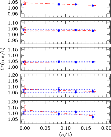
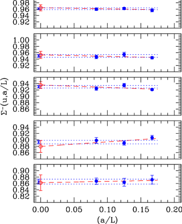
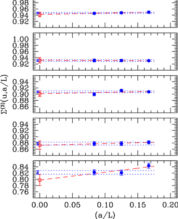
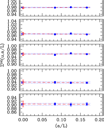
Since we do not implement $\mbox{O}(a)$ improvement of four-fermion operators, the only linear cutoff effects that are removed from $\Sigma(u,a/L)$ are those cancelled by the SW term in the fermion action. Therefore, we expect SSFs to approach the continuum limit linearly in $a/L$ and correspondingly we fit to the ansatz

$$\Sigma(u,a/L)=\sigma(u)+\rho(u)(a/L)\ .$$ (3.37)

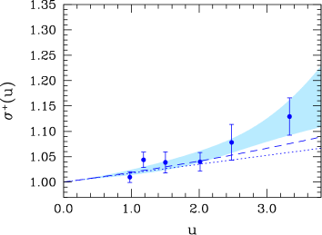
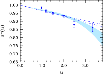
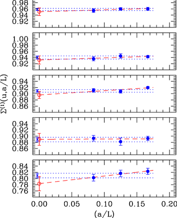
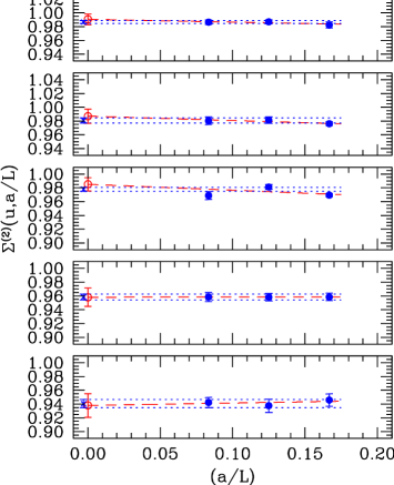
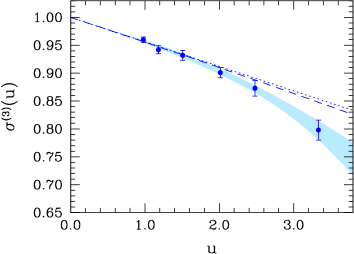
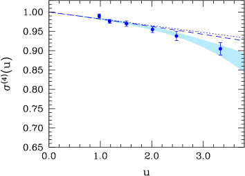
In practice it is often observed that the data corresponding to $L/a=8,12$ are compatible within errors, whereas the $L/a=6$ result, bearing the largest cutoff effects, is off. This suggests that, in analogy to [18], a weighted average of the two finest lattice results may be a reliable estimate of the continuum limit value. We have checked that, in most cases, linear fits to all three data-points and weighted averages of the two results from the finer lattices lead to continuum limit estimates, compatible within one standard deviation; cf. Figs. 2, 4 and 6. Fit results are reported in Table 2. Since the discretisation errors are ${\rm O}(a)$ and not ${\rm O}(a^{2})$ as in [18], we conservatively quote, as our best results, those obtained from linear extrapolations involving all three data-points.

It should be added that, besides the HYP2 action, we have also tried other static quark action varieties, namely the APE and the HYP1 ones (see ref. [20]), which differ from HYP2 by ${\rm O}(a^{2})$ lattice artefacts. Since the static four-quark operators are not $\mbox{O}(a)$ improved, it is reasonable to expect significant discretisation effects at the coarsest lattice spacing, which would enable combined fits of the data from all three actions, constrained to a common value in the continuum limit. Unsurprisingly, the situation turned out to be similar to that of [4], in that data obtained with the above actions do not differ noticeably (even at L/a = 6) and are very strongly correlated. Consequently, a combined continuum extrapolation affects the continuum limit results only marginally, with the relative error decreasing only by a few percent. For this reason we only quote results from the HYP2 analysis.

$u$	$\sigma^{+}(u)$	$\sigma^{-}(u)$	$\sigma^{(1)}(u)$	$\sigma^{(2)}(u)$	$\sigma^{(3)}(u)$	$\sigma^{(4)}(u)$
0.9793	1.010(11)	0.983(07)	0.946(08)	1.004(07)	0.960(05)	0.990(05)
1.1814	1.044(15)	0.965(10)	0.951(12)	0.991(08)	0.942(07)	0.976(05)
1.5078	1.039(21)	0.953(11)	0.932(13)	0.987(10)	0.932(09)	0.970(07)
2.0142	1.040(18)	0.936(11)	0.896(11)	0.985(10)	0.901(09)	0.955(08)
2.4792	1.078(35)	0.879(19)	0.890(19)	0.958(13)	0.873(14)	0.938(12)
3.3340	1.129(37)	0.862(25)	0.784(23)	0.938(17)	0.798(18)	0.905(16)

Table 2: Results of the continuum limit extrapolation of the lattice step-scaling functions $\Sigma^{\pm}$ and $\Sigma^{(k)}$. Data have been fitted from all available lattice resolutions as linear functions in $(a/L)$.

3.3 RG running in the continuum limit

In order to compute the RG running of the operators in the continuum limit as described in [18], the continuum SSFs have to be fitted to some functional form. The simplest choice is represented by a polynomial

$$\sigma(u)=1+s_{1}u+s_{2}u^{2}+s_{3}u^{3}+\dots\ ,$$ (3.38)

whose form is motivated by the perturbative series, with coefficients

$$s_{1}={\gamma}_{0}\ln 2\ ,$$ (3.39)

$$s_{2}={\gamma}_{1}\ln 2+\left[\frac{1}{2}(\gamma_{0})^{2}+b_{0}\gamma_{0}\right](\ln 2)^{2}\ .$$ (3.40)

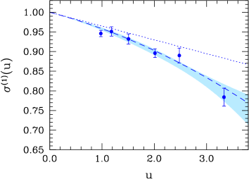
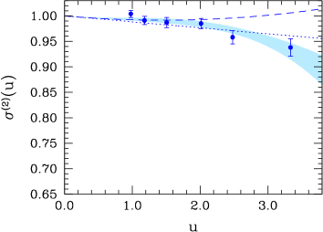
It is worth stressing that $s_{1}$ is universal and independent of $N_{\rm f}$, whereas $s_{2}$ carries a dependence upon $N_{\rm f}$ via $b_{0}$ and $\gamma_{1}$, with the latter coefficient introducing a scheme dependence. In our fits we truncated the polynomial at ${\rm O}(u^{3})$. The fits have been performed with $s_{1}$ fixed to its perturbative value and $s_{2}$, $s_{3}$ left as free parameters. Fit results are shown in Figs. 3, 5 and 7. Fitted values of $s_{2}$ turned out to be close to the perturbative prediction of Eq. (3.40), with the exception of ${\cal Q^{\prime}}_{2}^{+}$.

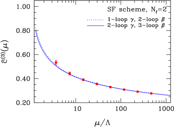
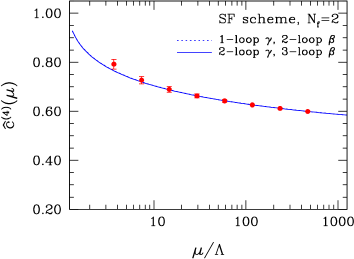
Once the continuous SSFs have been obtained as functions of the renormalised coupling, the ratios $\hat{c}$ (cf. Eq. (2.16)) are obtained recursively. The low-energy scale $\mu_{\rm had}=L_{\rm max}^{-1}$ is implicitly defined in this work through the condition $\kern 1.0pt\overline{\kern-1.0ptg\kern 0.0pt}\kern 1.0pt^{2}_{\rm\scriptscriptstyle SF}(L_{\rm max})=4.61$, as explained in [18]. This scale is chosen so that the renormalisation constants $Z(g_{0},a\mu_{\rm had})$ can be computed in the accessible $g_{0}$-range commonly used in large-volume simulations. The non-perturbative RG running of the six operators of interest are shown in Fig. 8.

$n$	$u$	$\hat{c}^{\,+}(L_{\rm max}^{-1})$	$\hat{c}^{\,-}(L_{\rm max}^{-1})$	$\hat{c}^{\,(1)}(L_{\rm max}^{-1})$	$\hat{c}^{\,(2)}(L_{\rm max}^{-1})$	$\hat{c}^{\,(3)}(L_{\rm max}^{-1})$	$\hat{c}^{\,(4)}(L_{\rm max}^{-1})$
0	4.610	1.246	0.551	0.807	0.680	0.524	0.776
1	3.032	1.225(26)	0.564(10)	0.775(14)	0.732(09)	0.532(08)	0.788(09)
2	2.341	1.212(38)	0.566(14)	0.773(20)	0.751(12)	0.538(11)	0.794(12)
3	1.918	1.205(46)	0.564(16)	0.773(24)	0.759(15)	0.541(13)	0.797(14)
4	1.628	1.202(53)	0.561(18)	0.772(27)	0.762(18)	0.541(14)	0.797(16)
5	1.414	1.201(60)	0.558(20)	0.772(30)	0.763(20)	0.541(15)	0.797(18)
6	1.251	1.201(66)	0.554(21)	0.771(33)	0.763(22)	0.540(17)	0.797(19)
7	1.121	1.202(71)	0.551(22)	0.770(35)	0.763(24)	0.539(18)	0.796(20)
8	1.017	1.202(76)	0.548(24)	0.770(37)	0.762(26)	0.538(19)	0.795(22)

Table 3: Perturbative matching (cf. Eq. (2.3)) for various choices of the matching scale $\mu_{\rm pt}=2^{n}\mu_{\rm had}$.

As discussed in our former quenched study [4], the main criterion for selecting robust schemes amounts to checking that the systematic uncertainty present in our final results, due to the NLO truncation of the perturbative matching at the scale $\mu_{\rm pt}\equiv 2^{n}\mu_{\rm had}$, is well under control. This in turn requires an estimate of the size of the NNLO contribution to $\hat{c}$. To this purpose we have re-computed ${\hat{c}}$ with two different ansätze for the NNLO anomalous dimensions ${\gamma}_{2}$: (i) we set $|{\gamma}_{2}/{\gamma}_{1}|=|{\gamma}_{1}/{\gamma}_{0}|$; (ii) we perform a two-parameter fit to the SSF with $s_{1}$,$s_{2}$ fixed to their perturbative values and $s_{3}$,$s_{4}$ left as free parameters, and then estimate ${\gamma}_{2}$ by equating the resulting value of $s_{3}$ to its perturbative expression

$$s_{3}=\gamma_{2}\ln 2 +\left[\gamma_{0}\gamma_{1}+2b_{0}\gamma_{1}+b_{1}\gamma_{0}\right](\ln 2)^{2}+$$

$$+\left[\frac{1}{6}\gamma_{0}^{3}+b_{0}\gamma_{0}^{2}+\frac{4}{3}b_{0}^{2}\gamma_{0}\right](\ln 2)^{3}\ .$$ (3.41)

The optimal schemes specified in Table 1 are precisely those for which the aforementioned determinations of the effective $\gamma_{2}$ lead to the smallest discrepancies between the corresponding universal factors $\hat{c}$.

The effect of varying the perturbative matching point in the optimal schemes is described by Table 3. We see that numbers are very stable for $n\geq 6$, while the uncertainty increases with $n$ due to progressive error accumulation at each step. Final results, reported in the second column of Table 7 refer to $n=7$. Note that typical relative errors are as big as 5%, which may result in a sizeable error in hadronic matrix elements, solely due to renormalisation.

4 Connection to hadronic observables

Having computed the universal evolution factors $\hat{c}(\mu_{\rm had})$, which provide the RG-running from the low energy matching scale $\mu_{\rm had}$ to a formally infinite one, we proceed to establish the connection between bare lattice operators and their RGI counterparts. The latter, defined in Eq. (2.16) from the integration of the Callan-Symanzik equation, are related to the bare operators used in lattice simulations via a total renormalisation factor $Z_{\rm\scriptscriptstyle RGI}(g_{0})$, defined as

$$Z_{\rm\scriptscriptstyle RGI}(g_{0})=Z(g_{0},a\mu_{\rm had})\hat{c}(\mu_{\rm had})\ .$$ (4.42)

The $Z_{\rm\scriptscriptstyle RGI}$ factor does not depend on any renormalisation scale and carries a dependence upon the renormalisation condition only via cutoff effects.

$\beta$	$\kappa$	$L/a$	$\kern 1.0pt\overline{\kern-1.0ptg\kern 0.0pt}\kern 1.0pt^{2}_{\rm\scriptscriptstyle SF}(L)$	$Z^{+}$	$Z^{-}$
5.20	0.13600	4	3.65(3)	0.7547(19)	0.4797(12)
		6	4.61(4)	0.7715(20)	0.4383(11)
5.29	0.13641	4	3.394(17)	0.7558(17)	0.5070(11)
		6	4.297(37)	0.7749(24)	0.4644(13)
		8	5.65(9)	0.8036(26)	0.4339(12)
5.40	0.13669	4	3.188(24)	0.7591(16)	0.5342(11)
		6	3.864(34)	0.7709(21)	0.4871(13)
		8	4.747(63)	0.7938(22)	0.4583(11)

Table 4: Results for $Z^{+}$ and $Z^{-}$ with $c_{\rm t}$ set to its 2–loop value. The values of $\kern 1.0pt\overline{\kern-1.0ptg\kern 0.0pt}\kern 1.0pt^{2}_{\rm\scriptscriptstyle SF}$ are from [26]. The hopping parameters $\kappa$ used in the simulations are the critical ones ($\kappa_{\rm cr}$) of [27].

$\beta$	$\kappa$	$L/a$	$\kern 1.0pt\overline{\kern-1.0ptg\kern 0.0pt}\kern 1.0pt^{2}_{\rm\scriptscriptstyle SF}(L)$	${\cal Z}^{(1)}$	${\cal Z}^{(2)}$	${\cal Z}^{(3)}$	${\cal Z}^{(4)}$
5.20	0.13600	4	3.65(3)	0.7793(17)	0.9741(16)	0.8681(16)	0.8317(13)
		6	4.61(4)	0.7118(17)	0.9409(15)	0.7857(13)	0.7921(13)
5.29	0.13641	4	3.394(17)	0.7862(16)	0.9766(16)	0.8768(15)	0.8397(14)
		6	4.297(37)	0.7275(20)	0.9431(18)	0.7992(16)	0.8017(15)
		8	5.65(9)	0.6612(19)	0.9150(16)	0.7337(15)	0.7619(14)
5.40	0.13669	4	3.188(24)	0.7972(15)	0.9805(14)	0.8864(14)	0.8497(12)
		6	3.864(34)	0.7378(18)	0.9434(17)	0.8098(15)	0.8094(14)
		8	4.747(63)	0.6840(16)	0.9231(14)	0.7529(13)	0.7781(12)

Table 5: Results for ${\cal Z}^{(k)}$ with $c_{\rm t}$ set to its 2–loop value. The values of $\kern 1.0pt\overline{\kern-1.0ptg\kern 0.0pt}\kern 1.0pt^{2}_{\rm\scriptscriptstyle SF}$ are from [26]. The hopping parameters $\kappa$ used in the simulations are the critical ones ($\kappa_{\rm cr}$) of [27].

In order to obtain $Z(g_{0},a\mu_{\rm had})$, we follow [18] and compute $Z(g_{0},a\mu)$ at three values of the lattice spacing, namely $\beta=\{5.20,5.29,5.40\}$, which belong to a range of inverse couplings commonly used for simulations of two-flavour QCD in physically large volumes. Simulation parameters and results are collected in Table 5 for the relativistic operators $Q_{1}^{\pm}$ and in Table 5 for the static ones ${\cal Q^{\prime}}_{k}^{+}$.

While the simulation at $(\beta=5.20,L/a=6)$ is exactly at the target value for $\kern 1.0pt\overline{\kern-1.0ptg\kern 0.0pt}\kern 1.0pt_{\rm\scriptscriptstyle SF}^{2}(L_{\rm max})$, corresponding to $Z(g_{0},a\mu_{\rm had})$, the simulations at the other $\beta$ values require a slight interpolation. We adopt a fit ansatz, motivated by Eq.(2.16),

$$\ln\left(Z\right)=c_{1}+c_{2}\ln(\kern 1.0pt\overline{\kern-1.0ptg\kern 0.0pt}\kern 1.0pt_{\rm\scriptscriptstyle SF}^{2})\;,$$ (4.43)

in order to interpolate the $Z$ factors between the values of $\kern 1.0pt\overline{\kern-1.0ptg\kern 0.0pt}\kern 1.0pt^{2}_{\rm\scriptscriptstyle SF}$ straddling the target value $\kern 1.0pt\overline{\kern-1.0ptg\kern 0.0pt}\kern 1.0pt_{\rm\scriptscriptstyle SF}^{2}(L_{\rm max})=4.61$. Note that the fits take into account the (independent) errors of both $Z$ and $\kern 1.0pt\overline{\kern-1.0ptg\kern 0.0pt}\kern 1.0pt_{\rm\scriptscriptstyle SF}^{2}$. Moreover, we have conservatively augmented the fit errors by the difference between the fit results of Eq. (4.43) and the results from a naive two-point linear interpolation in $\kern 1.0pt\overline{\kern-1.0ptg\kern 0.0pt}\kern 1.0pt_{\rm\scriptscriptstyle SF}^{2}$. The coefficients $c_{2}$ of the fits (4.43) deviate in a range of $7\%-30\%$ from the lowest order coefficients $\gamma_{0}/(2b_{0})$, signalling the presence of moderate higher-order perturbative effects.

$\beta$	$Z^{+}$	$Z^{+}_{\rm\scriptscriptstyle RGI}$		$Z^{-}$	$Z^{-}_{\rm\scriptscriptstyle RGI}$
5.20	0.7715(20)	0.927(2)(55)		0.4383(11)	0.241(1)(10)
5.29	0.7825(27)	0.940(3)(56)		0.4560(23)	0.251(1)(10)
5.40	0.7905(26)	0.950(3)(56)		0.4623(25)	0.255(1)(10)
$\beta$	${\cal Z}^{(1)}$	${\cal Z}^{(1)}_{\rm\scriptscriptstyle RGI}$		${\cal Z}^{(2)}$	${\cal Z}^{(2)}_{\rm\scriptscriptstyle RGI}$
5.20	0.7118(17)	0.548(1)(28)		0.9409(15)	0.718(1)(26)
5.29	0.7093(27)	0.546(2)(28)		0.9374(30)	0.715(2)(26)
5.40	0.6904(40)	0.532(3)(28)		0.9233(46)	0.704(4)(26)
$\beta$	${\cal Z}^{(3)}$	${\cal Z}^{(3)}_{\rm\scriptscriptstyle RGI}$		${\cal Z}^{(4)}$	${\cal Z}^{(4)}_{\rm\scriptscriptstyle RGI}$
5.20	0.7857(13)	0.423(1)(15)		0.7921(13)	0.631(1)(17)
5.29	0.7836(40)	0.422(2)(15)		0.7916(18)	0.630(1)(17)
5.40	0.7567(75)	0.408(4)(14)		0.7807(38)	0.621(3)(17)

Table 6: Results for $Z^{+}$, $Z^{-}$, ${\cal Z}^{(k)}$ and $Z^{+}_{\rm\scriptscriptstyle RGI}$, $Z^{-}_{\rm\scriptscriptstyle RGI}$, ${\cal Z}^{(k)}_{\rm\scriptscriptstyle RGI}$ for three bare gauge coupling values corresponding to our low-energy matching point at $\bar{g}^{2}_{\rm\scriptscriptstyle SF}=4.61$ in the SF scheme.

The resulting numbers for the renormalisation factors at the low energy matching scale, and also for the RGI renormalisation factors $Z_{\rm\scriptscriptstyle RGI}(g_{0})$, are collected in Table 6. The first error of the $Z_{\rm\scriptscriptstyle RGI}$’s stems from the error of $Z$ factors, whereas the second accounts for the uncertainties in the universal factors $\hat{c}$. Note that only the first of these errors should be added in quadrature to the error of the bare hadronic matrix elements, once these become available from future computations, in order to obtain the total error of the renormalised quantity, at a given lattice spacing. The second error, which is entirely unrelated to the discretisation of the theory, should only be added in quadrature to the continuum extrapolated hadronic matrix element. For the sake of convenience, a representation of the numerical results of Table 6 by interpolating polynomials is also adopted, i.e.

$$Z_{\rm\scriptscriptstyle RGI}=a_{0}+a_{1}(\beta-5.2)+a_{2}(\beta-5.2)^{2}\ ,$$ (4.44)

which can be used at any intermediate value of $\beta$ between $\beta=5.20$ and $\beta=5.40$. Fit coefficients are reported in Table 7 for the various operators. The uncertainty of the RGI constants at intermediate points may be easily obtained from those at the simulation points, see Table 6, by linear interpolation.

As a final remark, we observe that the simulation of the renormalisation factors at $\beta=5.20,L/a=4$ is not at the target value for $\bar{g}^{2}_{\rm\scriptscriptstyle SF}$. We used is as a check of the independence of the $Z_{\rm\scriptscriptstyle RGI}$, computed via Eq. (4.42) from the low energy matching scale. Specifically, the two measured values of $Z$-factors at $\beta=5.20$ have been used in order to extrapolate the renormalisation constants at $\bar{g}_{\rm\scriptscriptstyle SF}^{2}(L_{\rm max}/2)=3.0318$, where the non-perturbative matching with the universal evolution factors $\hat{c}$ has been subsequently performed. Results turned out to be fully compatible with those quoted in Table 6.

5 Conclusions

Using standard SF methods, we have performed a fully non-perturbative computation of the renormalisation and RG running of several four-fermion operators in $N_{\mathrm{\scriptstyle f}}=2$ QCD. We have considered the two operators made of four relativistic quark fields with a left-left Dirac structure and the complete basis of operators with two static and two relativistic quarks. The Wilson lattice actions have been implemented for both the gauge and the fermionic parts, the latter with a non-perturbatively tuned Clover term. The HYP2 discretisation of the static quark turned out to be the less noisy choice, after comparison with other options. Only the parity-odd parts of the operators have been analysed, as their renormalisation pattern is unaffected due to the loss of chiral symmetry by the regularisation.

$Q$	$\hat{c}(L_{\rm max}^{-1})$	$a_{0}$	$a_{1}$	$a_{2}$
$Q_{1}^{+}$	1.202(71)	0.9270	0.1741	-0.2973
$Q_{1}^{-}$	0.551(22)	0.2414	0.1431	-0.3853
${\cal Q^{\prime}}_{1}^{+}$	0.770(35)	0.5481	0.0285	-0.5546
${\cal Q^{\prime}}_{2}^{+}$	0.763(24)	0.7179	0.0010	-0.3407
${\cal Q^{\prime}}_{3}^{+}$	0.539(18)	0.4235	0.0411	-0.5962
${\cal Q^{\prime}}_{4}^{+}$	0.796(20)	0.6305	0.0291	-0.3723

Table 7: Universal factors $\hat{c}$ and coefficients of the interpolating polynomials of the RGI renormalisation constants, see Eq. (4.44). Uncertainties are discussed in the text.

Our results are an essential building block for any $N_{\mathrm{\scriptstyle f}}=2$ computation of quantities like $B_{K}$ and $B_{B}$. Nevertheless, their precision is somewhat limited by increased statistical fluctuations at the three strongest couplings and by the lack of a fourth, finer, lattice resolution which would improve the continuum extrapolation of the operator SSFs. This could lead to a potentially unsatisfactory total error on hadronic matrix elements. Future refinement (besides using a two–loop estimate of $c_{\rm t}$ throughout the runs and increased statistics at the three strongest couplings) is necessary, either by simulating closer to the continuum limit, or by completely removing leading order discretisation effects from the simulations.

$\kern 1.0pt\overline{\kern-1.0ptg\kern 0.0pt}\kern 1.0pt^{2}_{\rm\scriptscriptstyle SF}(L)$	$~{}~{}~{}~{}~{}\beta~{}~{}~{}~{}$	$~{}~{}~{}~{}~{}\kappa_{\rm cr}$	${L}/{a}$	${Z}^{+}\left(g_{0},{a}/{L}\right)$	${Z}^{+}\left(g_{0},{a}/{2L}\right)$	${\Sigma}^{+}\left(g_{0},{a}/{L}\right)$
0.9793	9.50000	0.131532	6	0.8714(14)	0.8827(22)	1.0129(30)
	9.73410	0.131305	8	0.8765(16)	0.8852(25)	1.0099(34)
	10.05755	0.131069	12	0.8899(17)	0.9022(52)	1.0138(61)
1.1814	8.50000	0.132509	6	0.8510(14)	0.8683(48)	1.0204(58)
	8.72230	0.132291	8	0.8594(29)	0.8849(33)	1.0296(52)
	8.99366	0.131975	12	0.8753(20)	0.9019(64)	1.0304(77)
1.5078	7.54200	0.133705	6	0.8309(18)	0.8580(47)	1.0327(60)
	7.72060	0.133497	8	0.8395(38)	0.8725(62)	1.0392(87)
1.5031	7.50000	0.133815	6	0.8317(15)	0.8390(55)	1.0088(69)
	8.02599	0.133063	12	0.8531(44)	0.8811(83)	1.0328(111)
2.0142	6.60850	0.135260	6	0.8023(19)	0.8382(32)	1.0448(47)
	6.82170	0.134891	8	0.8209(40)	0.8545(45)	1.0410(74)
	7.09300	0.134432	12	0.8400(44)	0.8771(70)	1.0442(100)
2.4792	6.13300	0.136110	6	0.7885(33)	0.8371(71)	1.0616(100)
	6.32290	0.135767	8	0.8038(31)	0.8466(127)	1.0531(163)
	6.63164	0.135227	12	0.8290(39)	0.8921(148)	1.0761(186)
3.3340	5.62150	0.136665	6	0.7667(45)	0.8193(129)	1.0686(179)
	5.80970	0.136608	8	0.7927(45)	0.8812(126)	1.1116(171)
	6.11816	0.136139	12	0.8252(68)	0.9040(110)	1.0955(161)
$\kern 1.0pt\overline{\kern-1.0ptg\kern 0.0pt}\kern 1.0pt^{2}_{\rm\scriptscriptstyle SF}(L)$	$~{}~{}~{}~{}~{}\beta~{}~{}~{}~{}$	$~{}~{}~{}~{}~{}\kappa_{\rm cr}$	${L}/{a}$	${Z}^{-}\left(g_{0},{a}/{L}\right)$	$\mathcal{Z}^{-}\left(g_{0},{a}/{2L}\right)$	${\Sigma}^{-}\left(g_{0},{a}/{L}\right)$
0.9793	9.50000	0.131532	6	0.7841(12)	0.7546(15)	0.9623(24)
	9.73410	0.131305	8	0.7767(10)	0.7500(27)	0.9657(37)
	10.05755	0.131069	12	0.7696(09)	0.7491(27)	0.9733(36)
1.1814	8.50000	0.132509	6	0.7512(11)	0.7185(34)	0.9564(47)
	8.72230	0.132291	8	0.7461(18)	0.7180(19)	0.9623(35)
	8.99366	0.131975	12	0.7372(10)	0.7075(30)	0.9598(43)
1.5078	7.54200	0.133705	6	0.7091(11)	0.6696(24)	0.9443(37)
	7.72060	0.133497	8	0.6998(18)	0.6680(44)	0.9547(68)
1.5031	7.50000	0.133815	6	0.7062(09)	0.6655(25)	0.9424(38)
	8.02599	0.133063	12	0.6954(25)	0.6584(31)	0.9468(56)
2.0142	6.60850	0.135260	6	0.6475(13)	0.5965(16)	0.9212(31)
	6.82170	0.134891	8	0.6428(27)	0.6011(25)	0.9351(55)
	7.09300	0.134432	12	0.6379(22)	0.5898(29)	0.9246(55)
2.4792	6.13300	0.136110	6	0.6029(21)	0.5470(37)	0.9072(69)
	6.32290	0.135767	8	0.5994(16)	0.5336(38)	0.8902(68)
	6.63164	0.135227	12	0.5995(22)	0.5386(53)	0.8984(94)
3.3340	5.62150	0.136665	6	0.5288(31)	0.4610(69)	0.8718(140)
	5.80970	0.136608	8	0.5363(24)	0.4632(63)	0.8637(124)
	6.11816	0.136139	12	0.5417(31)	0.4698(49)	0.8672(102)

Table 8: Numerical values of the renormalisation constants $Z^{+}$, $Z^{-}$ and the step scaling functions ${\Sigma}^{+}$, $\Sigma^{-}$ at various renormalised SF couplings and lattice spacings. Data at $\kern 1.0pt\overline{\kern-1.0ptg\kern 0.0pt}\kern 1.0pt^{2}_{\rm\scriptscriptstyle SF}=0.9793,\ 1.1814,\ 1.5031$ have been obtained with $c_{\rm t}$ evaluated in one-loop perturbation theory. The remaining data have been obtained with $c_{\rm t}$ evaluated in two-loop perturbation theory.

$\kern 1.0pt\overline{\kern-1.0ptg\kern 0.0pt}\kern 1.0pt^{2}_{\rm\scriptscriptstyle SF}(L)$	$~{}~{}~{}~{}~{}\beta~{}~{}~{}~{}$	$~{}~{}~{}~{}~{}\kappa_{\rm cr}$	${L}/{a}$	$\mathcal{Z}^{(1)}\left(g_{0},{a}/{L}\right)$	$\mathcal{Z}^{(1)}\left(g_{0},{a}/{2L}\right)$	${\Sigma}^{(1)}\left(g_{0},{a}/{L}\right)$
0.9793	9.50000	0.131532	6	0.8958(15)	0.8630(18)	0.9634(25)
	9.73410	0.131305	8	0.8845(13)	0.8486(23)	0.9594(29)
	10.05755	0.131069	12	0.8733(15)	0.8335(38)	0.9545(47)
1.1814	8.50000	0.132509	6	0.8771(16)	0.8421(41)	0.9601(50)
	8.72230	0.132291	8	0.8650(22)	0.8304(29)	0.9600(41)
	8.99366	0.131975	12	0.8503(17)	0.8117(47)	0.9545(59)
1.5078	7.54200	0.133705	6	0.8531(16)	0.8043(29)	0.9428(39)
	7.72060	0.133497	8	0.8385(34)	0.7924(53)	0.9450(74)
1.5031	7.50000	0.133815	6	0.8547(13)	0.8161(43)	0.9548(52)
	8.02599	0.133063	12	0.8161(43)	0.7638(37)	0.9359(67)
2.0142	6.60850	0.135260	6	0.8190(17)	0.7535(22)	0.9200(33)
	6.82170	0.134891	8	0.8082(31)	0.7334(35)	0.9075(56)
	7.09300	0.134432	12	0.7798(28)	0.7102(38)	0.9108(59)
2.4792	6.13300	0.136110	6	0.7937(27)	0.7085(49)	0.8927(68)
	6.32290	0.135767	8	0.7754(21)	0.6841(90)	0.8823(119)
	6.63164	0.135227	12	0.7492(25)	0.6691(65)	0.8931(92)
3.3340	5.62150	0.136665	6	0.7570(38)	0.6233(67)	0.8235(98)
	5.80970	0.136608	8	0.7330(37)	0.5987(71)	0.8168(106)
	6.11816	0.136139	12	0.7048(46)	0.5658(65)	0.8028(106)
$\kern 1.0pt\overline{\kern-1.0ptg\kern 0.0pt}\kern 1.0pt^{2}_{\rm\scriptscriptstyle SF}(L)$	$~{}~{}~{}~{}~{}\beta~{}~{}~{}~{}$	$~{}~{}~{}~{}~{}\kappa_{\rm cr}$	${L}/{a}$	$\mathcal{Z}^{(2)}\left(g_{0},{a}/{L}\right)$	$\mathcal{Z}^{(2)}\left(g_{0},{a}/{2L}\right)$	${\Sigma}^{(2)}\left(g_{0},{a}/{L}\right)$
0.9793	9.50000	0.131532	6	0.9810(11)	0.9645(15)	0.9832(19)
	9.73410	0.131305	8	0.9739(10)	0.9613(23)	0.9871(26)
	10.05755	0.131069	12	0.9676(09)	0.9627(37)	0.9949(39)
1.1814	8.50000	0.132509	6	0.9769(13)	0.9599(42)	0.9826(45)
	8.72230	0.132291	8	0.9699(18)	0.9572(21)	0.9869(28)
	8.99366	0.131975	12	0.9644(11)	0.9516(29)	0.9867(32)
1.5078	7.54200	0.133705	6	0.9738(11)	0.9507(25)	0.9762(28)
	7.72060	0.133497	8	0.9662(24)	0.9482(40)	0.9813(48)
1.5031	7.50000	0.133815	6	0.9707(11)	0.9579(24)	0.9868(28)
	8.02599	0.133063	12	0.9579(24)	0.9392(46)	0.9805(54)
2.0142	6.60850	0.135260	6	0.9667(12)	0.9371(18)	0.9694(22)
	6.82170	0.134891	8	0.9551(24)	0.9372(23)	0.9813(34)
	7.09300	0.134432	12	0.9476(22)	0.9179(49)	0.9687(56)
2.4792	6.13300	0.136110	6	0.9605(23)	0.9207(48)	0.9586(55)
	6.32290	0.135767	8	0.9496(14)	0.9099(51)	0.9582(56)
	6.63164	0.135227	12	0.9385(23)	0.8995(56)	0.9584(64)
3.3340	5.62150	0.136665	6	0.9511(41)	0.8997(75)	0.9459(89)
	5.80970	0.136608	8	0.9352(37)	0.8769(84)	0.9376(97)
	6.11816	0.136139	12	0.9200(35)	0.8669(59)	0.9423(74)

Table 9: Numerical values of the renormalisation constants $\mathcal{Z}^{(1)}$, $\mathcal{Z}^{(2)}$ and the step-scaling functions ${\Sigma}^{(1)}$, ${\Sigma}^{(2)}$ with HYP2 action at various renormalised SF couplings and lattice spacings. Data at $\kern 1.0pt\overline{\kern-1.0ptg\kern 0.0pt}\kern 1.0pt^{2}_{\rm\scriptscriptstyle SF}=0.9793,\ 1.1814,\ 1.5031$ have been obtained with $c_{\rm t}$ evaluated in one-loop perturbation theory. The remaining data have been obtained with $c_{\rm t}$ evaluated in two-loop perturbation theory.

$\kern 1.0pt\overline{\kern-1.0ptg\kern 0.0pt}\kern 1.0pt^{2}_{\rm\scriptscriptstyle SF}(L)$	$~{}~{}~{}~{}~{}\beta~{}~{}~{}~{}$	$~{}~{}~{}~{}~{}\kappa_{\rm cr}$	${L}/{a}$	$\mathcal{Z}^{(3)}\left(g_{0},{a}/{L}\right)$	$\mathcal{Z}^{(3)}\left(g_{0},{a}/{2L}\right)$	${\Sigma}^{(3)}\left(g_{0},{a}/{L}\right)$
0.9793	9.50000	0.131532	6	0.9306(10)	0.8879(13)	0.9541(17)
	9.73410	0.131305	8	0.9164(08)	0.8762(12)	0.9561(16)
	10.05755	0.131069	12	0.8973(07)	0.8586(21)	0.9569(24)
1.1814	8.50000	0.132509	6	0.9179(10)	0.8715(30)	0.9494(34)
	8.72230	0.132291	8	0.8996(13)	0.8526(17)	0.9478(23)
	8.99366	0.131975	12	0.8810(09)	0.8333(27)	0.9458(33)
1.5078	7.54200	0.133705	6	0.9038(10)	0.8411(20)	0.9307(25)
	7.72060	0.133497	8	0.8814(20)	0.8207(26)	0.9311(36)
1.5031	7.50000	0.133815	6	0.8998(10)	0.8564(20)	0.9517(25)
	8.02599	0.133063	12	0.8564(20)	0.7976(36)	0.9314(48)
2.0142	6.60850	0.135260	6	0.8794(12)	0.7981(16)	0.9075(22)
	6.82170	0.134891	8	0.8543(22)	0.7788(22)	0.9116(34)
	7.09300	0.134432	12	0.8231(22)	0.7405(37)	0.8997(50)
2.4792	6.13300	0.136110	6	0.8596(21)	0.7582(42)	0.8821(53)
	6.32290	0.135767	8	0.8347(13)	0.7329(52)	0.8780(63)
	6.63164	0.135227	12	0.7972(19)	0.6999(50)	0.8780(66)
3.3340	5.62150	0.136665	6	0.8346(36)	0.7043(62)	0.8439(83)
	5.80970	0.136608	8	0.7996(33)	0.6568(63)	0.8214(85)
	6.11816	0.136139	12	0.7587(30)	0.6241(58)	0.8227(82)
$\kern 1.0pt\overline{\kern-1.0ptg\kern 0.0pt}\kern 1.0pt^{2}_{\rm\scriptscriptstyle SF}(L)$	$~{}~{}~{}~{}~{}\beta~{}~{}~{}~{}$	$~{}~{}~{}~{}~{}\kappa_{\rm cr}$	${L}/{a}$	$\mathcal{Z}^{(4)}\left(g_{0},{a}/{L}\right)$	$\mathcal{Z}^{(4)}\left(g_{0},{a}/{2L}\right)$	${\Sigma}^{(4)}\left(g_{0},{a}/{L}\right)$
0.9793	9.50000	0.131532	6	0.9281(09)	0.9082(12)	0.9786(16)
	9.73410	0.131305	8	0.9213(08)	0.9033(12)	0.9804(15)
	10.05755	0.131069	12	0.9147(06)	0.9009(21)	0.9849(23)
1.1814	8.50000	0.132509	6	0.9158(10)	0.8950(24)	0.9773(28)
	8.72230	0.132291	8	0.9094(13)	0.8904(14)	0.9791(21)
	8.99366	0.131975	12	0.9022(08)	0.8811(19)	0.9766(23)
1.5078	7.54200	0.133705	6	0.8995(10)	0.8691(18)	0.9662(23)
	7.72060	0.133497	8	0.8924(18)	0.8668(28)	0.9714(37)
1.5031	7.50000	0.133815	6	0.8979(10)	0.8829(16)	0.9833(2)
	8.02599	0.133063	12	0.8829(16)	0.8536(28)	0.9668(36)
2.0142	6.60850	0.135260	6	0.8749(11)	0.8353(14)	0.9548(20)
	6.82170	0.134891	8	0.8671(19)	0.8321(18)	0.9597(30)
	7.09300	0.134432	12	0.8562(18)	0.8143(31)	0.9510(42)
2.4792	6.13300	0.136110	6	0.8566(19)	0.8006(36)	0.9347(47)
	6.32290	0.135767	8	0.8461(14)	0.7906(41)	0.9344(51)
	6.63164	0.135227	12	0.8360(17)	0.7832(46)	0.9368(58)
3.3340	5.62150	0.136665	6	0.8268(35)	0.7474(58)	0.9040(80)
	5.80970	0.136608	8	0.8142(30)	0.7337(63)	0.9011(85)
	6.11816	0.136139	12	0.8002(26)	0.7239(48)	0.9046(67)

Table 10: Numerical values of the renormalisation constants $\mathcal{Z}^{(3)}$, $\mathcal{Z}^{(4)}$ and the step-scaling functions ${\Sigma}^{(3)}$, ${\Sigma}^{(4)}$ with HYP2 action at various renormalised SF couplings and lattice spacings. Data at $\kern 1.0pt\overline{\kern-1.0ptg\kern 0.0pt}\kern 1.0pt^{2}_{\rm\scriptscriptstyle SF}=0.9793,\ 1.1814,\ 1.5031$ have been obtained with $c_{\rm t}$ evaluated in one-loop perturbation theory. The remaining data have been obtained with $c_{\rm t}$ approximated in two-loop perturbation theory.

Figure 2: Continuum extrapolation of the SSFs for $Q_{1}^{+}$ (left) and $Q_{1}^{-}$ (right). The renormalised coupling increases from top to bottom. Blue dotted lines and the blue cross at $a/L=0$ correspond to weighted averages of the $L/a=8,12$ data, red dashed lines and the red $a/L=0$ open point to linear extrapolations in $a/L$ of the three data.

Figure 3: The step-scaling functions $\sigma^{+}$ and $\sigma^{-}$ (discrete points) as obtained non-perturbatively. The shaded area is the one sigma band obtained by fitting the points to a polynomial as discussed in the text. The dotted (dashed) line is the LO (NLO) perturbative result.

Figure 4: Continuum extrapolation of the SSFs for ${{\cal Q}^{\prime}}_{1}^{+}$ (left) and ${{\cal Q}^{\prime}}_{2}^{+}$ (right). The renormalised coupling increases from top to bottom. Blue dotted lines and the blue cross at $a/L=0$ correspond to weighted averages of the $L/a=8,12$ data, red dashed lines and the red $a/L=0$ open point to linear extrapolations in $a/L$ of the three data.

Figure 5: The step-scaling functions $\sigma^{(1)}$ and $\sigma^{(2)}$ (discrete points) as obtained non-perturbatively. The shaded area is the one sigma band obtained by fitting the points to a polynomial as discussed in the text. The dotted (dashed) line is the LO (NLO) perturbative result.

Figure 6: Continuum extrapolation of the SSFs for ${{\cal Q}^{\prime}}_{3}^{+}$ (left) and ${{\cal Q}^{\prime}}_{4}^{+}$ (right). The renormalised coupling increases from top to bottom. Blue dotted lines and the blue cross at $a/L=0$ correspond to weighted averages of the $L/a=8,12$ data, red dashed lines and the red $a/L=0$ open point to linear extrapolations in $a/L$ of the three data.

Figure 7: The step-scaling functions $\sigma^{(3)}$ and $\sigma^{(4)}$ (discrete points) as obtained non-perturbatively. The shaded area is the one sigma band obtained by fitting the points to a polynomial as discussed in the text. The dotted (dashed) line is the LO (NLO) perturbative result.

Figure 8: RG-running of of the four-quark operators obtained non-perturbatively (discrete points) at specific values of the renormalisation scale $\mu$, in units of $\Lambda$. The lines are perturbative results at the order shown for the Callan-Symanzik $\beta$ function and the operator anomalous dimension $\gamma$.

References

- [1] A. Jüttner, PoS LAT2007 (2007) 014, arXiv:0711.1239 [hep-lat]; M. Della Morte, PoS LAT2007 (2007) 008, arXiv:0711.3160 [hep-lat]; W. Lee, PoS LAT2006 (2006) 015, [arXiv:hep-lat/0610058]; T. Onogi, PoS LAT2006 (2006) 017, [arXiv:hep-lat/0610115].
- [2] M. Guagnelli et al., JHEP 0603 (2006) 088, [arXiv:hep-lat/0505002].
- [3] F. Palombi, C. Pena and S. Sint, JHEP 0603 (2006) 089, [arXiv:hep-lat/0505003].
- [4] F. Palombi et al., JHEP 0709 (2007) 062, arXiv:0706.4153 [hep-lat].
- [5] P. Dimopoulos et al., PoS LAT2006 (2006) 158, [arXiv:hep-lat/0610077]; P. Dimopoulos et al., PoS LAT2007 (2007) 368, arXiv:0710.2862 [hep-lat].
- [6] P. Dimopoulos et al., Nucl. Phys. B 749 (2006) 69, [arXiv:hep-ph/0601002].
- [7] P. Dimopoulos et al., Nucl. Phys. B 776 (2007) 258, [arXiv:hep-lat/0702017]; C. Pena, PoS LAT2006 (2006) 019, [arXiv:hep-lat/0610109].
- [8] P. Dimopoulos et al., Phys. Lett. B 641 (2006) 118, [arXiv:hep-lat/0607028].
- [9] A. Donini et al., Eur. Phys. J. C 10, 121 (1999), [arXiv:hep-lat/9902030].
- [10] F. Palombi et al., JHEP 0608 (2006) 017, [arXiv:hep-lat/0604014].
- [11] C. W. Bernard et al., Nucl. Phys. Proc. Suppl. 4 (1988) 483.
- [12] R. Frezzotti et al., JHEP 0108 (2001) 058, [arXiv:hep-lat/0101001].
- [13] M. Della Morte et al., Nucl. Phys. B 713 (2005) 378, [arXiv:hep-lat/0411025].
- [14] M. Lüscher et al. Nucl. Phys. B 478 (1996) 365, [arXiv:hep-lat/9605038].
- [15] M. Golterman and E. Pallante, JHEP 0110 (2001) 037, [arXiv:hep-lat/0108010]; M. Golterman and E. Pallante, Phys. Rev. D 74 (2006) 014509, [arXiv:hep-lat/0602025].
- [16] S. Capitani et al., Nucl. Phys. B 544 (1999) 669, [arXiv:hep-lat/9810063].
- [17] R. Sommer, [arXiv:hep-lat/0611020].
- [18] M. Della Morte et al., Nucl. Phys. B 729 (2005) 117, [arXiv:hep-lat/0507035].
- [19] K. Jansen and R. Sommer, Nucl. Phys. B 530 (1998) 185 [Erratum-ibid. B 643 (2002) 517], [arXiv:hep-lat/9803017].
- [20] M. Della Morte, A. Shindler and R. Sommer, JHEP 0508, 051 (2005), [arXiv:hep-lat/0506008].
- [21] E. Eichten and B. R. Hill, Phys. Lett. B 234 (1990) 511.
- [22] A. Hasenfratz and F. Knechtli, Phys. Rev. D 64 (2001) 034504, [arXiv:hep-lat/0103029].
- [23] M. Lüscher et al., Nucl. Phys. B 384 (1992) 168, [arXiv:hep-lat/9207009].
- [24] A. Bode, P. Weisz and U. Wolff, Nucl. Phys. B 576 (2000) 517 [Erratum-ibid. B 600 (2001 ERRAT,B608,481.2001) 453], [arXiv:hep-lat/9911018].
- [25] U. Wolff, Comput. Phys. Commun. 156 (2004) 143 [Erratum-ibid. 176 (2007) 383], [arXiv:hep-lat/0306017].
- [26] M. Della Morte et al., Nucl. Phys. B 713, 378 (2005), [arXiv:hep-lat/0411025].
- [27] M. Göckeler et al., Phys. Lett. B 639 (2006) 307, [arXiv:hep-ph/0409312].