Strains and Jets in black hole fields

Abstract

We study the behaviour of an initially spherical bunch of particles emitted along trajectories parallel to the symmetry axis of a Kerr black hole. We show that, under suitable conditions, curvature and inertial strains compete to generate jet-like structures.

1 Introduction

In recent papers, Bini, de Felice and Geralico (2006, 2007) considered how the relative deviations among the particles of a given bunch depend on the geometric properties of the frame adapted to a fiducial observer. Here we outline the main steps of their analysis which revealed how spacetime curvature and inertial strains compete to generate jet-like structures.

2 The relative deviation equation

Consider a bunch of test particles, i.e. a congruence ${\mathcal{C}}_{U}$ of timelike world lines with unit tangent vector $U$ ($U\cdot U=-1$) parametrized by the proper time $\tau_{U}$. In general, the lines of the congruence ${\mathcal{C}}_{U}$ are accelerated with acceleration $a(U)=\nabla_{U}U$. Let ${\mathcal{C}}_{*}$ be a fixed world line of the congruence which we consider as that of the “fiducial observer.” The separation between the line ${\mathcal{C}}_{*}$ and a line of ${\mathcal{C}}_{U}$ is represented by a connecting vector $Y$, i.e. a vector undergoing Lie transport along $U$, namely $\pounds_{U}Y=0$. The latter equation becomes:

$$\dot{Y}\equiv\frac{{\rm D}Y}{{\rm d}\tau_{U}}=\nabla_{Y}U=-(Y\cdot U)a(U)-K(U)\mathop{\hbox{\vrule width=0.5pt,height=6.0pt\vrule height=0.5pt,width=6.0pt}}Y\ ,$$ (1)

where the kinematical tensor $K(U)$ is defined as $K(U)=\omega(U)-\theta(U)$. Here the antisymmetric tensor $\omega(U)^{\beta}{}_{\alpha}$ represents the vorticity of the congruence ${\mathcal{C}}_{U}$ and the symmetric tensor $\theta(U)^{\beta}{}_{\alpha}$ represents the expansion. The symbol $\mathop{\hbox{\vrule width=0.5pt,height=6.0pt\vrule height=0.5pt,width=6.0pt}}$ stands for right-contraction operation among tensors. The covariant derivative along $U$ of both sides of the Lie transport equation gives rise to the “relative deviation equation” which, once projected on a given spatial triad $E_{a}$, reads:

$$\ddot{Y}^{a}+{\mathcal{K}}_{(U,E)}{}^{a}{}_{b}Y^{b}=0\ ,$$ (2)

where ${\mathcal{K}}_{(U,E)}{}^{a}{}_{b}=[T_{({\rm fw},U,E)}-S(U)+{\mathcal{E}}(U)]^{a}{}_{b}$. Here ${\mathcal{E}}(U)$ is the electric part of the Riemann tensor relative to $U$ namely ${\mathcal{E}}(U)^{\alpha}{}_{\gamma}=R^{\alpha}{}_{\beta\gamma\delta}U^{\beta}U^{\delta}$. The strain tensor $S$ is defined as

$$S(U)_{ab}=\nabla(U)_{b}a(U)_{a}+a(U)_{a}a(U)_{b}\ ;$$ (3)

$S(U)$ depends only on the congruence ${\cal C}_{U}$ and not on the chosen spatial triad $E_{a}$, while the tensor $T$, given by:

$$T_{({\rm fw},U,E)}{}^{a}{}_{b}=\delta^{a}_{b}\omega_{({\rm fw},U,E)}^{2}-\omega_{({\rm fw},U,E)}^{a}\omega_{({\rm fw},U,E)}{}_{b}$$

$$\quad-\epsilon^{a}{}_{bf}\dot{\omega}_{({\rm fw},U,E)}^{f}-2\epsilon^{a}{}_{fc}\omega_{({\rm fw},U,E)}^{f}K(U)^{c}{}_{b}\ ,$$ (4)

as derived in detail in Bini et al. (2006), characterizes the given frame relative to a Fermi-Walker frame along the congruence. We like to stress here that the components of the deviation vector should be restricted to the reference observer’s world line; they may behave differently according to the reference frame set up for their measurements.

3 Axial observers in Kerr spacetime

Consider Kerr spacetime, whose line element in Kerr-Schild coordinates $(t,x^{1}=x,x^{2}=y,x^{3}=z)$ is given by

$${\rm d}s^{2} = g_{\alpha\beta}{\rm d}x^{\alpha}{\rm d}x^{\beta}\equiv(\eta_{\alpha\beta}+2Hk_{\alpha}k_{\beta}){\rm d}x^{\alpha}{\rm d}x^{\beta}\ ,$$ (5)

where $H=\mathcal{M}r^{3}/(r^{4}+a^{2}z^{2})$, $\eta_{\alpha\beta}$ is the flat spacetime metric and

$$k_{\alpha}{\rm d}x^{\alpha}=-{\rm d}t-\frac{(rx+ay){\rm d}x+(ry-ax){\rm d}y}{r^{2}+a^{2}}-\frac{z}{r}{\rm d}z\ ,$$ (6)

with $r$ implicitly defined by

$$\frac{x^{2}+y^{2}}{r^{2}+a^{2}}+\frac{z^{2}}{r^{2}}=1\ .$$ (7)

Here $\mathcal{M}$ and $a$ are the total mass and specific angular momentum characterizing the spacetime. Consider now a set of particles moving along the $z$-direction, on and nearby the axis of symmetry, with four velocity

$$U=\gamma[m+\nu E(m)_{\hat{3}}]\ ,\qquad\gamma=(1-\nu^{2})^{-1/2}\ ,$$ (8)

where $m=\sqrt{(z^{2}+a^{2})/\Delta_{z}}\partial_{t}$, $E(m)_{\hat{3}}=\sqrt{\Delta_{z}/(z^{2}+a^{2})}[\partial_{z}+(2{\mathcal{M}}z/\Delta_{z})\partial_{t}]$, $\Delta_{z}=z^{2}-2{\mathcal{M}}z+a^{2}$ and where the instantaneous linear velocity $\nu=\nu(z)$, relative to the local static observers, is function of $z$. These particles are accelerated except perhaps those which move strictly on the axis of symmetry. Their history forms a congruence ${\mathcal{C}}_{U}$ of $\infty^{2}$ world lines and each of them can be parametrized by the pair $(x,y)$ of the spatial coordinates. A frame adapted to this kind of orbits was found explitely in Bini at al. (2007) and termed $\{E(U)_{\hat{a}}\}$. The congruence is accelerated with non-vanishing components along the three spatial directions $E(U)_{\hat{a}}$. It is now possible to study the components of the vector $Y$ connecting a specific curve of the congruence which we fix along the rotation axis with $x=0=y$ with tangent vector $\tilde{U}$ and nearby world lines of the same congruence. The reference world line is accelerated along the direction $E(\tilde{U})_{\hat{3}}$, i.e. $a(\tilde{U})=a(\tilde{U})^{\hat{3}}E(\tilde{U})_{\hat{3}}$, with

$$a(\tilde{U})^{\hat{3}} = \frac{{\rm d}}{{\rm d}z}\left(\frac{\gamma}{\sqrt{\tilde{g}_{33}}}\right)\ ,$$ (9)

where $\tilde{g}_{33}=(z^{2}+a^{2})/\Delta_{z}$ denotes the restriction on the axis of that metric coefficient.

4 Tidal forces, frame induced deformations and strains

In order to determine the deviations measured by the “fiducial observer” $\tilde{U}$ with respect to the chosen frame we need to evaluate the kinematical fields of the congruence, namely the acceleration $a(U)$, the vorticity $\omega(U)$ and the expansion $\theta(U)$), the electric part of the Weyl tensor ${\mathcal{E}}(U)$, the strain tensor $S(U)$ and the characterization of the spatial triad $\{E(U)_{\hat{a}}\}$ with respect to a Fermi-Walker frame given by the tensor $T_{({\rm fw},U,E)}$. All these quantities are calculated on the axis of symmetry so we can drop the tilde ($\,\tilde{}\,$); a lengthy calculation leads to the following results.
i) The only nonvanishing components of the kinematical tensors $\omega(U)$ and $\theta(U)$ are given by

$$\theta(U)_{\hat{3}\hat{3}}=\frac{{\rm d}}{{\rm d}z}\left(\frac{\gamma\nu}{\sqrt{g_{33}}}\right)\ ,\ \omega(U)_{\hat{1}\hat{2}}=\gamma(1+\nu)\frac{2a\mathcal{M}z}{\sqrt{\Delta_{z}}(z^{2}+a^{2})^{3/2}}\ .$$ (10)

ii) The vorticity vector becomes $\omega_{({\rm fw},U,E)}=\omega_{({\rm fw},U,E)}{}_{\hat{3}}E(U)_{\hat{3}}$ with $\omega_{({\rm fw},U,E)}{}_{\hat{3}}=\omega(U)_{\hat{1}\hat{2}}$.
iii) The electric part of the Weyl tensor is a diagonal matrix with respect to the adapted frame $\{E(U)_{\hat{a}}\}$, namely

$${\mathcal{E}}(U)=\mathcal{M}z\frac{z^{2}-3a^{2}}{(z^{2}+a^{2})^{3}}\,{\rm diag}\left[1,1,-2\right]\ .$$ (11)

iv) The only nonvanishing components of the tensor $T_{({\rm fw},U,E)}$ turn out to be

$$T_{({\rm fw},U,E)}{}_{\hat{1}\hat{1}}=T_{({\rm fw},U,E)}{}_{\hat{2}\hat{2}}=-\omega_{({\rm fw},U,E)}{}_{\hat{3}}^{2}\ ,$$

$$T_{({\rm fw},U,E)}{}_{\hat{1}\hat{2}}=-T_{({\rm fw},U,E)}{}_{\hat{2}\hat{1}}=-\dot{\omega}_{({\rm fw},U,E)}{}_{\hat{3}}$$

$$=\frac{\gamma\nu}{\sqrt{g_{33}}}\frac{{\rm d}}{{\rm d}z}\omega_{({\rm fw},U,E)}{}_{\hat{3}}\ .$$ (12)

v) The non-zero components of the strain tensor $S(U){}^{\hat{a}}{}_{\hat{b}}$ can be written as

$$S(U){}_{\hat{1}\hat{1}} = S(U){}_{\hat{2}\hat{2}}=-\omega_{({\rm fw},U,E)}{}_{\hat{3}}^{2}+\mathcal{M}z\frac{z^{2}-3a^{2}}{(z^{2}+a^{2})^{3}}\ ,$$

$$S(U){}_{\hat{1}\hat{2}} = -S(U){}_{\hat{2}\hat{1}}=-\dot{\omega}_{({\rm fw},U,E)}{}_{\hat{3}}\ ,$$

$$S(U){}_{\hat{3}\hat{3}} = \frac{\gamma}{\sqrt{g_{33}}}\frac{{\rm d}}{{\rm d}z}[a(U)^{\hat{3}}]+[a(U)^{\hat{3}}]^{2}\ .$$ (13)

From Eqs. (11)–(4) it follows that the deviation matrix ${\mathcal{K}}_{(U,E)}$ has only the non-zero component

$${\mathcal{K}}_{(U,E)}{}_{\hat{3}\hat{3}}=-\frac{\gamma}{\sqrt{g_{33}}}\frac{{\rm d}[a(U)^{\hat{3}}]}{{\rm d}z}-[a(U)^{\hat{3}}]^{2}+{\mathcal{E}}(U)_{\hat{3}\hat{3}}\ ;$$ (14)

hence, as expected, the particles emitted nearby the axis in the $z$-direction will be relatively accelerated in the $z$-direction only. The spatial components of the connecting vector $Y$ are then obtained by integrating the deviation equation (2) which now reads

$$\ddot{Y}^{\hat{1}}=0\ ,\quad\ddot{Y}^{\hat{2}}=0\ ,\quad\ddot{Y}^{\hat{3}}=-{\mathcal{K}}_{(U,E)}{}_{\hat{3}\hat{3}}Y^{\hat{3}}\ .$$ (15)

Equations (15) can be analytically integrated to give

$$Y^{\hat{1}}=Y^{\hat{1}}_{0},\qquad Y^{\hat{2}}=Y^{\hat{2}}_{0},\qquad Y^{\hat{3}}=C\frac{\gamma\nu}{\sqrt{g_{33}}}\ ,$$ (16)

where $C$ is a constant. This result shows that the conditions imposed on the particles of the bunch to move parallel to the axis of rotation is assured by a suitable balancing among the gravitoelectric (curvature) tensor (11), the inertial tensor (4) and the strain tensor (4).

5 Reference world line uniformly accelerated

Let us now consider the case of the reference world line with tangent vector $U$ constantly accelerated, namely with $a(U)^{\hat{3}}=A=\,\,$const. The instantaneous linear velocity relative to a local static observer is given by

$$\nu_{A}=\left[1-\frac{1}{g_{33}[\bar{\kappa}+A(z-z_{0})]^{2}}\right]^{1/2}\ ,$$ (17)

where the positive value has been selected for $\nu_{A}$ in order to consider outflows. $\bar{\kappa}$ is a constant which acquires the meaning of the conserved (Killing) energy of the particle if the latter is not accelerated. The solution of equation (16) is given by

$$Y^{\hat{1}}=Y^{\hat{1}}_{0}\ ,\qquad Y^{\hat{2}}=Y^{\hat{2}}_{0}\ ,\qquad Y^{\hat{3}}=Y^{\hat{3}}_{0}\frac{\gamma_{A}\nu_{A}}{\sqrt{g_{33}}\bar{\kappa}\nu_{A}^{0}}\ ,$$ (18)

where $\nu_{A}^{0}=\nu_{A}(z_{0})$. Figure 1 shows the behaviour of an initially spherical bunch of particles in the $Y^{\hat{1}}$-$Y^{\hat{3}}$ plane for increasing values of the coordinate $z$. We clearly see a stretching along the $z$ axis leading to a collimated axial outflow of matter, clearly suggestive of an “astrophysical jet.” Figure 2 shows qualitatively the behaviour of an initially spherical bunch of particles. Note that in this case the acceleration acts contrarily to the curvature tidal effect; indeed, $S(U)$, $T_{({\rm fw},U,E)}$ and ${\mathcal{E}}(U)$ act in competition leading to a quite unexpected result. It is easy to show that the stretching shown in Figs. 1 and 2 for uniformly accelerated outgoing particles persists also with a general acceleration. Moreover this behaviour does not depend of the acceleration mechanism itself. Observed jets (see Figs. 3 and 4 as an example) appear to contain spherical bunches of particles emerging from the central black hole.

Figure 1: An initially circular bunch of particles on the $y^{\hat{1}}$-$y^{\hat{3}}$ plane emitted along the $z$-axis at $z_{0}/\mathcal{M}=2$ is shown to spread for the choice of parameters $a/\mathcal{M}=0.5$, $\bar{\kappa}=1.5$ and ${\mathcal{M}}\,A=0.3$ as an example. The curves correspond to increasing values of the coordinate $z/\mathcal{M}=[2,4,6,8,10,12,14,16,18,20]$.

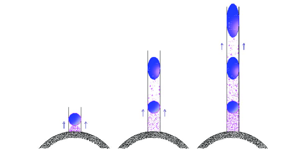
Figure 2: The qualitative behaviour of an initially spherical bunch of particles moving out along the axis of a rotating black hole.

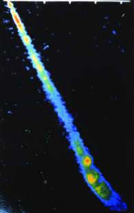
Figure 3: The jet from the Galaxy M87 (Credit:J.A. Biretta et al. Hubble Heritage Team (STScl/AURA), NASA) We can see almost spherical bunches of particles along the jet.

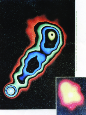
Figure 4: Details of the jet from M87 close to the central black hole (Credit:J.A. Biretta et al. Hubble Heritage Team (STScl/AURA), NASA). Here we see a spherical bunch of particles apparently emerging from nearby the hole.

References

- [1] D. Bini, F. de Felice, and A. Geralico, Class. Quantum Grav. 23, 7603 (2006).
- [2] D. Bini, F. de Felice, and A. Geralico, Phys. Rev. D 76, 047502 (2007).