Theory of electronic transport in random alloys with short-range order: Korringa-Kohn-Rostoker non-local coherent potential approximation

Abstract

We present an ab-initio formalism for the calculation of transport properties in compositionally disordered systems within the framework of the Korringa-Kohn-Rostoker non-local coherent potential approximation. Our formalism is based upon the single-particle Kubo-Greenwood linear response and provides a natural means of incorporating the effects of short-range order upon the transport properties. We demonstrate the efficacy of the formalism by examining the effects of short-range order and clustering upon the transport properties of disordered $AgPd$ and $CuZn$ alloys.

I Introduction

The Korringa-Kohn-Rostoker coherent potential approximation (KKR-CPA) cpa represents an extremely successful one-electron theory capable of describing the properties of many compositionally disordered alloy systems. In particular, in combination with density functional theory (DFT) dft1 ; dft2 ; johnson ; johnson-totalE and the Korringa-Kohn-Rostoker method of band theory gyorffy ; stocks ; gyorffy2 , it provides a fully first-principles description of such systems. A long history of successful applications staunton ; luders ; faulkner ; gyorffy3 ; hughes ; MAEvsT attests to the utility and accuracy to which the method is capable.

Of particular relevance to our discussion here, the KKR-CPA has been used to calculate the transport properties of such alloys. Historically, the early work concerning this topic involved the use of a Boltzmann equation butler1 ; butler2 ; butler3 , and although these works demonstrated remarkable agreement with experiment, they did suffer from two notable defects: namely, the requirement that well-defined energy bands exist within the alloy, and the neglect of vertex, or “scattering-in”, terms. The former defect limits the application of such a theory to weak-scattering alloys only, while the latter could be expected to lead to significant error in systems such as those where appreciable s-p or s-d scattering manifests itself.

Velicky velicky developed a CPA theory for transport using the Kubo-Greenwood Kubo ; Greenwood formalism as his starting point, which was applied to a two-level tight-binding Hamiltonian. Although capable of yielding vertex corrections, this approach suffered from difficulties when applied to realistic systems. For example, the necessity of assuming that the wavefunctions are identical on all lattice sites, irrespective of the occupying atomic species. The seminal work of Butler butler4 , resolved these issues, as he developed a KKR-CPA theory based upon the Kubo-Greenwood linear response formalism Kubo ; Greenwood . As a multiple-scattering based approach, this did not require the existence of well-defined energy bands, and further, Butler demonstrated how the vertex corrections arose quite naturally within his formalism. Although the formal developments of this work followed Velicky’s quite closely, the use of a realistic single-electron muffin-tin Hamiltonian allowed connection with first-principles methods to be made. The method has been applied with success to a range of alloy systems swihart ; banhart and it has also been successfully extended to the relativistic regime banhart2 .

Of course, all of these calculations suffer from the main drawback of the CPA; namely that as a single-site mean-field theory, it is incapable of incorporating the effects of local-environment fluctuations in the alloy crystal potential. The CPA therefore explicitly ignores the effects of such short-range order (SRO) effects upon the physics of disordered alloys. As discussed by Gonis gonis , these statistical fluctuations can be important. Whilst in general the presence of SRO is likely to diminish the resistivity there are examples, the so-called “Komplex” K-state alloys K-state , where the onset of SRO is accompanied by an increase in the alloy residual resistivity.

Recently there have been some successful attempts at calculating the effects of SRO upon the electronic structure of disordered alloys and they provide the means to study transport properties. Mookerjee and Prasad mookerjee ; dasgupta ; dasgupta2 , using a TB-LMTO method tb in conjunction with an augmented space formalism mookerjee2 ; kaplan and real space recursion method haydock described SRO effects on alloy electronic densities of states and related quantities whilst Saha et al. saha have obtained spectral functions within the same framework. Recently Tarafder et al. Tarafder have developed a formalism for the optical conductivity and reflectivity from the same basis and used it to study copper-zinc alloys. To date however it has not been possible to incorporate this technique fully within electronic density functional theory. The recent work of Rowlands et al derwyn ; derwyn2 ; derwyn dft , along with Biava et al. biava ; biava2 concern a development which is not restricted in this way. References derwyn, ; derwyn2, formulate and illustrate a successful method for incorporating the effects of SRO within the framework of KKR-CPA theory, whilst implementation for realistic systems is described in references derwyn2, ; biava, . The method can be readily combined with density functional theory to provide a first principles description of disordered alloys as demonstrated in reference derwyn dft, ; r-nlcpa, . This nonlocal CPA (NLCPA) theory is based upon reciprocal space coarse-graining ideas introduced by Jarrell and Krishnamurthy jarrell and krishnamurthy originating from the dynamical cluster approximation (DCA) hettler ; hettler2 ; maier . The KKR-NLCPA derwyn ; derwyn2 introduces an effective (translationally invariant) disorder term $\delta G$ which represents an effective propagator that accounts for all nonlocal scattering correlations on the electronic propagation due to disorder configurations and modifies the structure constants accordingly. By coarse-graining reciprocal space, one naturally introduces real space periodically repeating clusters. As such, the NLCPA maps an effective lattice problem to that of an impurity cluster embedded in a self-consistently determined effective medium, and thus yields a cluster generalisation of the KKR-CPA that includes non-local correlations up to the range of the cluster size. Unlike other cluster approaches, such as the molecular CPA (MCPA) tsukada it is fully translationally invariant, that is, the effective medium has the site-to-site translational invariance of the underlying lattice. It is also computationally tractable, largely on account of the reciprocal space coarse-graining procedure employed.

Thus far, the NLCPA has been employed to investigate the effects of SRO upon the electronic structure of a range of realistic systems, using both the muffin-tin Hamiltonian derwyn2 ; spectral , and the tight-binding approach gary . Given its ability to address such issues successfully and its proven incorporation into an electronic density functional theory derwyn dft (DFT) for disordered systems with SRO it makes sense then to extend it to the calculation of transport properties. To this end, by invoking time dependent DFT  TDDFT within the adiabatic approximation, in this paper we present a formalism for the determination of the residual resistivity in the KKR-NLCPA, and explicitly demonstrate the efficacy of the method through application to several realistic alloy systems. Our theoretical formalism is a careful generalisation of that of Butler butler4 and where appropriate we omit the steps in the derivation which can be straightforwardly obtained from this paper. Our paper is structured as follows: The next section gives a short overview of the conductivity tensor and then the transport coefficients available from the Kubo-Greenwood formalism. This is followed by a section containing the salient points of the KKR-NLCPA formalism including its use in implementing the density functional theory. We then develop our theory for the conductivity of disordered systems with short-range order which includes the treatment of ‘vertex corrections’. The implementation strategy is outlined before calculations for the effects of SRO on the resistivity of both b.c.c. $CuZn$ and f.c.c. $AgPd$ are presented.

II The Conductivity; Kubo-Greenwood linear response

The Kubo-Greenwood Kubo ; Greenwood linear response formalism states that, for disordered system, the symmetric part of the conductivity tensor has coefficients $C$ which can be determined from the evaluation of an expression of the form

$$C=\mbox{Tr}<O_{1}GO_{2}G>,$$ (1)

where $G$ is a single-particle Green’s function, which is dependent upon the details of the effective one-electron potential. $O_{1}$ and $O_{2}$ are operators, and the angled brackets denote a configuration average over the distribution of the potentials.

To determine the d.c. conductivity, we consider the following expression  Kubo ; Greenwood ; butler4

$$\sigma_{\mu\nu}(E_{F})=\frac{\pi\hbar}{N\Omega}\bigg{<}\sum_{mn}J_{mn;\mu}J_{nm;\nu}\delta(E_{F}-E_{m})\delta(E_{F}-E_{n})\bigg{>},$$ (2)

where $J_{mn;\mu}=\langle m|J_{\mu}|n\rangle$ denotes the matrix element of the current operator in the $\mu$th spatial direction, which is given by

$$J_{\mu}=-i\hbar\frac{e}{m}\frac{\partial}{\partial r_{\mu}},$$ (3)

with $|m\rangle$ and $|n\rangle$ denoting eigenfunctions of a particular configuration of the disordered system. Here, $N$ is the number of atoms, and $\Omega$ is the volume per atom. $E_{F}$ is the Fermi energy.

Within the KKR approach, the electronic structure of the alloy is expressed in terms of the single-particle Green’s function, rather than in terms of eigenstates and eigenvalues of the Hamiltonian; we can introduce the Green’s function simply by using the identity henry

$$-\pi\sum_{n}|n\rangle\langle n|\delta(E-E_{n})=\lim_{\eta\to 0}\mbox{Im}G(E+i\eta),$$ (4)

while the awkward imaginary part of the Green’s function may be removed by writing

$$-2i\pi\sum_{n}|n\rangle\langle n|\delta(E-E_{n})=\lim_{\eta\to 0}[G(E+i\eta)-G(E-i\eta)].$$ (5)

Inserting this into Eq. (2), yields the following for the conductivity

$$\sigma_{\mu\nu} = 1/4\lim_{\eta\to 0}[\tilde{\sigma}_{\mu\nu}(E^{+},E^{+})-\tilde{\sigma}_{\mu\nu}(E^{-},E^{+})-$$ (6)

$$\tilde{\sigma}_{\mu\nu}(E^{+},E^{-})+\tilde{\sigma}_{\mu\nu}(E^{-},E^{-})]$$

where we define the complex energies as

$$E^{+}=E_{F}+i\eta,\>E^{-}=E_{F}-i\eta,\>\eta\to 0$$ (7)

and

$$\tilde{\sigma}_{\mu\nu}(z_{1},z_{2})=-\frac{\hbar}{\pi N\Omega}\mbox{Tr}<J_{\mu}G(z_{1})J_{\nu}G(z_{2})>,$$ (8)

where $z_{1}$ and $z_{2}$ are each either $E^{+}$ or $E^{-}$.

For non-overlapping effective single electron potentials the Hamiltonian takes the form

$$H=-\frac{\hbar^{2}}{2m}\nabla^{2}+\sum_{i}v_{\gamma}(\mathbf{r}-\mathbf{R}_{i}),$$ (9)

where the atomic positions $\mathbf{R}_{i}$ are fixed, and form a regular lattice. The potentials $v_{\gamma}(\mathbf{r}_{i})$ vary from site to site ($\mathbf{r}_{i}=\mathbf{r}-\mathbf{R}_{i}$) and $\gamma$ is a configuration label.

Within the multiple-scattering theory, the single-particle Green’s function for a given configuration $\gamma$ can be written as faulkner and stocks

$$G_{\gamma}(E,\mathbf{r}_{i},\mathbf{r}^{\prime}_{j})=2m/\hbar^{2}\bigg{(}\sum_{\Lambda,\Lambda^{\prime}}Z^{i}_{\Lambda,\gamma}(E,\mathbf{r}_{i})\tau^{ij}_{\gamma;\Lambda,\Lambda^{\prime}}Z^{j,\dagger}_{\Lambda^{\prime},\gamma}(E,\mathbf{r}^{\prime}_{j})-\sum_{\Lambda}Z^{i}_{\Lambda,\gamma}(\mathbf{r}^{<}_{i})J^{i,\dagger}_{\Lambda,\gamma}(E,\mathbf{r}^{>}_{i})\delta_{ij}\bigg{)},$$ (10)

where $\tau^{ij}_{\gamma,\Lambda,\Lambda^{\prime}}$ is the scattering path operator (SPO) describing propagation between sites $i$ and $j$ in configuration $\gamma$, $Z^{i}_{\Lambda,\gamma}(E,\mathbf{r}_{i})$ is the regular solution to the Schrödinger/Dirac equation in the cell surrounding the atom $i$, and $J^{i}_{\Lambda,\gamma}(E,\mathbf{r}^{\prime}_{i})$ represents the irregular solution within the same cell (note that there should be no confusion with the current matrix elements here). $\Lambda$ encapsulates the appropriate angular momentum quantum numbers. butler4 ; banhart2

In calculating the conductivity, the second term in the Green’s function expression (Eq.( 10)) is real and may be omitted, when calculated for a real potential at a real energy butler4 . Thus the conductivity may be written

$$\tilde{\sigma}_{\mu\nu}(z_{1},z_{2})=-\frac{4m^{2}}{\pi N\Omega\hbar^{3}}\sum_{i,j}\sum_{\Lambda_{1},\Lambda_{2},\Lambda_{3},\Lambda_{4}}<J^{i,\gamma}_{\Lambda_{1}\Lambda_{2},\mu}(z_{2},z_{1})\tau^{ij}_{\gamma;\Lambda_{2}\Lambda_{3}}(z_{1})J^{j,\gamma}_{\Lambda_{3}\Lambda_{4},\nu}(z_{1},z_{2})\tau^{ji}_{\gamma;\Lambda_{4}\Lambda_{1}}(z_{2})>$$ (11)

with

$$J^{i,\gamma}_{\Lambda\Lambda^{\prime},\mu}(z,z^{\prime})=-\frac{ie\hbar}{m}\int_{cell_{i}}d\mathbf{r}_{i}Z^{i}_{\Lambda,\gamma}(\mathbf{r}_{i},z)\frac{\partial}{\partial r_{\mu}}Z^{i}_{\Lambda^{\prime},\gamma}(\mathbf{r}_{i},z^{\prime})$$ (12)

where $cell_{i}$ defines the region surrounding the site $i$.

We now need to consider how to carry out the averaging over configurations implicit in Eq.(11). Butler butler4 showed in detail how to use the CPA to accomplish this. The single site nature of this effective medium theory means, however, that the potentials on the different lattices could only be treated as statistically independent. We will show how to carry out the averaging using the NLCPA whereby short-ranged correlations can be naturally included. To this end in the next section we summarise briefly the key aspects we need from the KKR-NLCPA together with its incorporation into electronic density functional theory. Full details can be found in references derwyn, ; derwyn2, ; derwyn dft, ; r-nlcpa, .

III The KKR-NLCPA and Electronic Density Functional Theory

In general the scattering path operator (SPO) between two sites $i$ and $j$ for an electron, moving through an effective medium so that it mimicks the average motion in a disordered system, is given by

$$\hat{\tau}^{ij}=\hat{t}\,\delta_{ij}+\sum_{k\neq i}\hat{t}\,(G(\mathbf{R}_{i}-\mathbf{R}_{k})+\delta\hat{G}(\mathbf{R}_{i}-\mathbf{R}_{k}))\hat{\tau}^{kj}.$$ (13)

Here, all quantities are matrices in angular momentum space and the indices $i$,$j$ run over all sites in the lattice. The $G(\mathbf{R}_{i}-\mathbf{R}_{k})$’s are structure constants. The effective medium is specified by single site t-matrices $\hat{t}$ and effective structure constant corrections $\delta\hat{G}(\mathbf{R}_{i}-\mathbf{R}_{j})$. The effective medium must be translationally invariant so that $\hat{\tau}^{ij}$ is given in terms of a Brillouin zone integral.

$$\hat{\tau}^{ij}=\frac{1}{\Omega_{BZ}}\int_{\Omega_{BZ}}d\mathbf{k}[\hat{t}^{-1}-G(\mathbf{k})-\delta\hat{G}(\mathbf{k})]^{-1}e^{i\mathbf{k}\cdot(\mathbf{R}_{i}-\mathbf{R}_{j})}.$$ (14)

In order to establish a tractable procedure for determining the effective medium the NLCPA draws its chief idea from the dynamical cluster approximation (DCA) for interacting electron systems hettler ; jarrell and krishnamurthy . This is a coarse graining of $\delta\hat{G}$ consistently in real and reciprocal space and a mapping to a self-consistently embedded impurity cluster problem with appropriate boundary conditions imposed gary . The full translational symmetry of the underlying lattice is preserved. The size of the cluster sets the range of correlations that can be included. The lattice is divided into ‘tiles’ centred on a superlattice vectors $\mathbf{R}_{C}$ and each contains $N_{c}$ sites at positions $\mathbf{R}_{C}+\mathbf{R}_{I},I=1,\cdots N_{c}$. The Brillouin zone is also broken into $N_{c}$ tiles, of volume $\Omega_{t}=\Omega_{BZ}/N_{c}$, centred on the cluster momenta $\mathbf{K}_{n},n=1,\cdots N_{c}$ and the $\mathbf{R}_{I}$’s and $\mathbf{K}_{n}$ satisfy the following equation:

$$\frac{1}{N_{c}}\sum_{\mathbf{K}_{n}}e^{i\mathbf{K}_{n}\cdot(\mathbf{R}_{I}-\mathbf{R}_{J})}=\delta_{IJ}.$$ (15)

$\delta\hat{G}(\mathbf{k})$ is coarse-grained so that it has the average value $\delta\hat{G}(\mathbf{K}_{n})$ in a tile centred on $\mathbf{K}_{n}$ and in real space, $\delta\hat{G}(\mathbf{R}_{I}-\mathbf{R}_{J})=(1/N_{c})\sum_{\mathbf{K}_{n}}\delta\hat{G}(\mathbf{K}_{n})e^{i\mathbf{K}_{n}\cdot(\mathbf{R}_{I}-\mathbf{R}_{J})}$ with $\delta\hat{G}(\mathbf{K}_{n})=\sum_{J\neq I}\delta\hat{G}(\mathbf{R}_{I}-\mathbf{R}_{J})e^{-i\mathbf{K}_{n}\cdot(\mathbf{R}_{I}-\mathbf{R}_{J})}$.

The SPO is coarse-grained,

$$\hat{\tau}(\mathbf{K}_{n})=\frac{N_{c}}{\Omega_{BZ}}\int_{\Omega_{t}}d\tilde{\mathbf{k}}[\hat{t}^{-1}-G(\tilde{\mathbf{k}}+\mathbf{K}_{n})-\delta\hat{G}(\mathbf{K}_{n})]^{-1}$$ (16)

appropriate to the reciprocal space tile of volume $\Omega_{t}$ and in real space for multiple scattering starting and ending on cluster sites $I$ and $J$ respectively.

$$\hat{\tau}^{IJ}=\frac{1}{\Omega_{BZ}}\sum_{\mathbf{K}_{n}}(\int_{\Omega_{t}}d\tilde{\mathbf{k}}[\hat{t}^{-1}-G(\tilde{\mathbf{k}}+\mathbf{K}_{n})-\delta\hat{G}(\mathbf{K}_{n})]^{-1})e^{i\mathbf{K}_{n}\cdot(\mathbf{R}_{I}-\mathbf{R}_{J})}.$$ (17)

Note how $e^{i\tilde{\mathbf{k}}\cdot(\mathbf{R}_{I}-\mathbf{R}_{J})}$ is taken to be $\approx 1$ as the coarse graining is applied hettler . The final step is to find the SPO for an impurity cluster, $\tau^{IJ}_{\gamma}$ describing a particular configuration $\gamma_{C}$ of atoms which is embedded into the NLCPA medium. By demanding that the average is equal to the SPO of the NLCPA enables the effective t-matrix and structure constant corrections to be determined, i.e.,

$$\sum_{\gamma_{C}}P_{\gamma_{C}}\tau^{IJ}_{\gamma_{C}}=\hat{\tau}^{IJ}.$$ (18)

Short-range order, SRO, can be included by choosing the probabilities $P_{\gamma_{C}}$ appropriately as demonstrated in, for example, refs. derwyn2, ; derwyn dft, .

In ref. derwyn dft, , in a generalisation of the work of Johnson et al. johnson ; johnson-totalE , it is described how to specify a configurationally averaged electronic Grand potential, $\bar{\Omega}$ in terms of KKR-NLCPA quantities and charge densities $\rho_{\gamma_{C}}(\mathbf{r}_{I})$ and one-electron potentials, $v_{\gamma_{C}}(\mathbf{r}_{I})$ different for each cluster configuration. The functional minimisation of $\bar{\Omega}$ with respect to the charge densities, $\rho_{\gamma_{C}}(\mathbf{r}_{I})$’s, determines the total energy of the system and requires the $\rho_{\gamma_{C}}(\mathbf{r}_{I})$’s and $v_{\gamma_{C}}(\mathbf{r}_{I})$ ’s to be found self-consistently. Rowlands et al derwyn dft applied this DFT to investigate how the total energy, charge densities and densities of states are affected by SRO. Tulip et al. spectral showed how further information can be found about the effects of SRO on the electronic structure by formulating and calculating the Bloch spectral function at the cluster momenta and averaged over tiles whilst Batt and Rowlands gary explained how the spectral function at any point in the Brillouin zone can be found. In the following we build on these developments and describe the theory for a two-particle correlation function of disordered system with SRO. The particular example is to the d.c. conductivity.

IV Analytic configuration averaging of the conductivity using the KKR-NLCPA

From the above it is clear that the KKR-NLCPA should enable an analytical configurational average of the conductivity to be carried out. To do so, some care needs to be exercised. There are two distinct cases that we must consider in Eq.(11): (i) where the two sites under consideration, $i$ and $j$, lie within the same NLCPA cluster, and (ii) when they lie in two different clusters, in which case the occupancies of the sites will be statistically independent, as the two distinct clusters will be statistically independent. This is a natural generalisation of Butler’s work butler4 , where he distinguishes between the two cases of $i=j$ and $i\neq j$.

Hereon we use lower case letters to denote general sites in the lattice,$i,j,\cdots$; upper case $C$ denotes tiles containing the clusters; and upper case letters, with the exception of $C$, denote sites within clusters. So for a site at position $\mathbf{R}_{i}$ we use $\mathbf{R}_{i}=\mathbf{R}_{C}+\mathbf{R}_{I}$ and $I,J,\cdots$ label sites within tile $C$, $I^{\prime},J^{\prime},\cdots$ sites within tile $C^{\prime}$ etc.

We accordingly write

$$\tilde{\sigma}_{\mu\nu}(z_{1},z_{2})=\tilde{\sigma}^{0}_{\mu\nu}(z_{1},z_{2})+\tilde{\sigma}^{1}_{\mu\nu}(z_{1},z_{2})$$ (19)

$$\tilde{\sigma}^{0}_{\mu\nu}(z_{1},z_{2})=-\frac{4m^{2}}{\pi\hbar^{3}\Omega}\sum_{J\in C}\sum_{\Lambda_{1},\Lambda_{2},\Lambda_{3},\Lambda_{4}}<J^{I}_{\Lambda_{1}\Lambda_{2};\mu}(z_{2},z_{1})\tau^{IJ}_{\Lambda_{2}\Lambda_{3}}(z_{1})J^{J}_{\Lambda_{3}\Lambda_{4};\nu}(z_{1},z_{2})\tau^{JI}_{\Lambda_{4}\Lambda_{1}}(z_{2})>$$ (20)

and

$$\tilde{\sigma}^{1}_{\mu\nu}(z_{1},z_{2})=-\frac{4m^{2}}{\pi\hbar^{3}\Omega}\sum_{C^{\prime}\neq C}\sum_{J^{\prime}\in C^{\prime}}\sum_{\Lambda_{1},\Lambda_{2},\Lambda_{3},\Lambda_{4}}<J^{I}_{\Lambda_{1}\Lambda_{2};\mu}(z_{2},z_{1})\tau^{I,C^{\prime}+J^{\prime}}_{\Lambda_{2}\Lambda_{3}}(z_{1})J^{J^{\prime}}_{\Lambda_{3}\Lambda_{4};\nu}(z_{1},z_{2})\tau^{C^{\prime}+J^{\prime},I}_{\Lambda_{4}\Lambda_{1}}(z_{2})>$$ (21)

where $\tilde{\sigma}^{0}$ includes sites $J$ within the same NLCPA cluster (denoted $C$) as our reference site $I$, and $\tilde{\sigma}^{1}$ includes all sites lying outside this cluster. Note that in writing these equations, we have utilised the translational invariance of the averaged system to remove the second sum appearing in Eq.(11).

We now introduce response functions such that we can write

$$\tilde{\sigma}^{0}_{\mu\nu}(z_{1},z_{2})=-\frac{4m^{2}}{\pi\hbar^{3}\Omega}\sum_{\gamma_{C}}P_{\gamma_{C}}\sum_{\Lambda_{1},\Lambda_{2}}J^{I,\gamma_{C}}_{\Lambda_{1}\Lambda_{2};\mu}(z_{2},z_{1})K^{I;C,\gamma_{C}}_{\Lambda_{2},\Lambda_{1};\nu}(z_{1},z_{2})$$ (22)

$$K^{I;C,\gamma_{C}}_{\Lambda_{2},\Lambda_{1};\nu}(z_{1},z_{2})=\sum_{J\in C}\sum_{\Lambda_{3},\Lambda_{4}}<\tau^{IJ}_{\Lambda_{2}\Lambda_{3}}(z_{1})J^{J,\gamma_{C},\nu}_{\Lambda_{3}\Lambda_{4}}(z_{1},z_{2})\tau^{JI}_{\Lambda_{4}\Lambda_{1}}(z_{2})>_{C,\gamma_{C}}.$$ (23)

$K^{I;C,\gamma_{C}}_{\Lambda_{2},\Lambda_{1};\nu}(z_{1},z_{2})$ involves an average over all configurations except the configuration is fixed in cluster $C$ to be $\gamma_{C}$. The single site quantity $J^{I,\gamma_{C},}_{\Lambda_{1}\Lambda_{2};\mu}(z_{2},z_{1})$ is set up depending on what kind of element occupies site $I$ and the one-electron potential $v_{\gamma_{C}}(\mathbf{r}_{I})$ that is dependent on the configuration $\gamma_{C}$.

Similarly, for the inter-cluster contributions to the conductivity, we can introduce the following

$$\tilde{\sigma}^{1}_{\mu\nu}(z_{1},z_{2})=-\frac{4m^{2}}{\pi\hbar^{3}\Omega}\sum_{C^{\prime}\neq C}\sum_{\gamma_{C}}P_{\gamma_{C}}\sum_{\gamma_{C^{\prime}}}P_{\gamma_{C^{\prime}}}\sum_{\Lambda_{1},\Lambda_{2}}J^{I,\gamma_{C}}_{\Lambda_{1}\Lambda_{2};\mu}(z_{2},z_{1})L^{I,C,\gamma_{C};C^{\prime},\gamma_{C^{\prime}}}_{\Lambda_{2},\Lambda_{1};\nu}(z_{1},z_{2})$$ (24)

and

$$L^{I,C,\gamma_{C};C^{\prime},\gamma_{C^{\prime}}}_{\Lambda_{2},\Lambda_{1};\nu}(z_{1},z_{2})=\sum_{J^{\prime}\in C^{\prime}}\sum_{\Lambda_{3},\Lambda_{4}}<\tau^{I,C^{\prime}+J^{\prime}}_{\Lambda_{2}\Lambda_{3}}(z_{1})J^{J^{\prime},\gamma_{C^{\prime}}}_{\Lambda_{3}\Lambda_{4};\nu}(z_{1},z_{2})\tau^{C^{\prime}+J^{\prime},I}_{\Lambda_{4}\Lambda_{1}}(z_{2})>_{C,\gamma_{C};C^{\prime},\gamma_{C^{\prime}}}$$ (25)

where the notation is similar to before but the average now fixes cluster $C$ to be occupied by configuration $\gamma_{C}$ and cluster $C^{\prime}$ to be loaded with configuration $\gamma_{C^{\prime}}$.

In order to evaluate the ensemble averages contained in Eqs.(22)-(25) it is helpful to express the SPO, $\tau$, for a particular configuration as the SPO in the NLCPA medium plus corrections. Again this is the direct generalisation of Butler’s approach butler4 . We can write

$$\tau^{ij}=\hat{\tau}^{ij}+\sum_{k,l}\hat{\tau}^{ik}T^{kl}\hat{\tau}^{lj}$$ (26)

where the effective medium path SPO is denoted $\hat{\tau}$ as before and $T$ is the total scattering matrix relevant to the specific configuration. The double summation is taken over all lattice sites. $\tau^{ij}$ satisfies the following equation

$$\sum_{k}(t^{-1}_{k}\delta_{ik}-G(\mathbf{R}_{i}-\mathbf{R}_{k}))\tau^{kj}=\delta_{ij}$$ (27)

where all quantities are matrices in angular momentum space. We consider fluctuations about the NLCPA medium to obtain

$$\sum_{k}\bigg{(}(t^{-1}_{k}-\hat{t}^{-1})\delta_{ik}+\delta\hat{G}(\mathbf{R}_{i}-\mathbf{R}_{k})+\hat{t}^{-1}-\delta\hat{G}(\mathbf{R}_{i}-\mathbf{R}_{k})-G(\mathbf{R}_{i}-\mathbf{R}_{k})\bigg{)}\tau^{kj}=\delta_{ij}$$ (28)

which can be re-arranged to yield

$$\tau^{ij}=\hat{\tau}^{ij}-\sum_{k,l}\hat{\tau}^{ik}\Delta m^{kl}\tau^{lj}.$$ (29)

with

$$\Delta m^{kl}=(t^{-1}_{k}-\hat{t}^{-1})\delta_{kl}-\delta\hat{G}(\mathbf{R}_{k}-\mathbf{R}_{l})$$ (30)

and have used the fact that the effective medium SPO may be written as the inverse of the matrix with elements $(\hat{t}^{-1}\,\delta_{ij}-\delta\hat{G}(\mathbf{R}_{i}-\mathbf{R}_{j})-G(\mathbf{R}_{i}-\mathbf{R}_{j}))$.

We can thus write down

$$\sum_{l}T^{kl}\hat{\tau}^{lj}=\sum_{l}\Delta m^{kl}\tau^{lj}.$$ (31)

If we now substitute for $\tau^{lj}$ using Eq.( 26), label the sites according to clusters, $C$ and sites within those clusters (uppercase letters), we obtain

$$T^{C+K,C^{\prime}+L^{\prime}}=x^{KL}\delta_{C,C^{\prime}}+\sum_{C^{\prime\prime}\neq C}\sum_{MN^{\prime\prime}}x^{KM}\hat{\tau}^{C+M,C^{\prime\prime}+N^{\prime\prime}}T^{C^{\prime\prime}+N^{\prime\prime},C^{\prime}+L^{\prime}}$$ (32)

where we have introduced the matrix $x$ associated with a single cluster of sites, given by

$$x^{IJ}=\sum_{K}\bigg{(}1+\Delta m\,\hat{\tau}\bigg{)}^{-1}_{IK}\Delta m^{KJ}.$$ (33)

Our results here are a direct cluster generalisation of Butler’s butler4 . Note also that these results are consistent with Hwang et al’s cluster CPA conductivity formalism hwang (although that is phrased in terms of $t$-matrices, rather than the $x$-matrix that we use in this work). Further, the special case of a single-site cluster recovers the more familiar CPA results.

The NLCPA amounts to writing

$$<T^{C+K,C^{\prime}+L^{\prime}}>_{NLCPA}=<x^{KL}>\delta_{C,C^{\prime}}+\sum_{C^{\prime\prime}\neq C}\sum_{MN^{\prime\prime}}<x^{KM}>\hat{\tau}^{C+M,C^{\prime\prime}+N^{\prime\prime}}<T^{C^{\prime\prime}+N^{\prime\prime},C^{\prime}+L^{\prime}}>_{NLCPA}$$ (34)

and if we choose that $<x^{IJ}>=0$, which is another way of expressing the NLCPA ansatz (Eq. (18)) then $<T>_{NLCPA}=0$, and we obtain $<\tau>_{NLCPA}=\hat{\tau}$, (Eq. (18)). Of course, in writing this, we have made the approximation that

$$<x^{KM}\hat{\tau}^{C+M,C^{\prime\prime}+N^{\prime\prime}}T^{C^{\prime\prime}+N^{\prime\prime},C^{\prime}+L^{\prime}}>\approx<x^{KM}>\hat{\tau}^{C+M,C^{\prime\prime}+N^{\prime\prime}}<T^{C^{\prime\prime}+N^{\prime\prime},C^{\prime}+L^{\prime}}>$$ (35)

which is analogous to the usual CPA-type averaging approximation.

Using Eq. (26) and closely following a cluster generalisation of Butler’s analogous derivation, which refers to fluctuations about the single site CPA medium, we find (suppressing angular momentum labelling)

$$K^{I;C,\gamma_{C}}_{\nu}=\sum_{M,N}D^{\gamma_{C}}_{IM}\tilde{K}_{MN;\nu}^{C,\gamma_{C}}D^{\dagger\gamma_{C}}_{NI}$$ (36)

with

$$\tilde{K}_{IJ;\nu}^{C,\gamma_{C}}=\sum_{KL}\hat{\tau}^{IK}\tilde{J}_{KL;\nu}^{\gamma_{C}}\hat{\tau}^{LJ}+\sum_{C^{\prime\prime}\neq C}\sum_{K^{\prime\prime},L^{\prime\prime}}\hat{\tau}^{I,C^{\prime\prime}+K^{\prime\prime}}\Gamma^{C,\gamma_{C}}_{C^{\prime\prime};K^{\prime\prime}L^{\prime\prime};\nu}\hat{\tau}^{C^{\prime\prime}+L^{\prime\prime},J}$$ (37)

and

$$L^{I,C,\gamma_{C};C^{\prime}\gamma_{C^{\prime}}}_{\nu}=\sum_{M,N}D^{\gamma_{C}}_{IM}\tilde{L}_{MN;\nu}^{C,\gamma_{C};C^{\prime},\gamma_{C^{\prime}}}D^{\dagger\gamma_{C}}_{NI}$$ (38)

where

$$\tilde{L}_{MN;\nu}^{C,\gamma_{C};C^{\prime},\gamma_{C^{\prime}}} = \sum_{K^{\prime},L^{\prime}}\hat{\tau}^{M,C^{\prime}+K^{\prime}}\tilde{J}^{\gamma_{C^{\prime}}}_{K^{\prime}L^{\prime};\nu}\hat{\tau}^{C^{\prime}+L^{\prime}}$$ (39)

$$+\sum_{C^{\prime\prime}\neq(C,C^{\prime})}\sum_{K^{\prime\prime},L^{\prime\prime}}(\hat{\tau}^{M,C^{\prime\prime}+K^{\prime\prime}}\Gamma^{C,\gamma_{C};C^{\prime},\gamma_{C^{\prime}}}_{C^{\prime\prime},K^{\prime\prime},L^{\prime\prime};\nu}\hat{\tau}^{C^{\prime\prime}+L^{\prime\prime},N}).$$

In Eqs. (36) and (38) we use the NLCPA projector $D$($D^{\dagger}$) which is $D=(1+\Delta m\hat{\tau})^{-1}$ ($(1+\hat{\tau}\Delta m)$) found in Eqs. (30) and (33). The NLCPA ansatz can be re-written in terms of them, i.e. $\sum_{\gamma_{C}}P_{\gamma_{C}}D^{\gamma_{C}}=1$. We have also defined the current quantities

$$\tilde{J}^{\gamma_{C}}_{KL;\nu}=\sum_{N}D^{\dagger\gamma_{C}}_{KN}J^{N,\gamma_{C}}_{\nu}D^{\gamma_{C}}_{NL}.$$ (40)

in Eqs.(37) and (39). Finally we have introduced vertex functions $\Gamma^{C,\gamma_{C}}_{C^{\prime\prime},K^{\prime\prime},L^{\prime\prime};\nu}$, $\Gamma^{C,\gamma_{C};C^{\prime},\gamma_{C^{\prime}}}_{C^{\prime\prime},K^{\prime\prime},L^{\prime\prime};\nu}$ which are the NLCPA analogues of the vertex functions derived by Butler butler4 . We now show how to calculate these quantities.

V Vertex Functions and the Conductivity

Our two vertex functions are slightly different. $\Gamma^{C,\gamma_{C}}_{C^{\prime\prime};K^{\prime\prime},L^{\prime\prime};\nu}$, which appears in Eq.(37) for the intra-cluster component of the conductivity, concerns the connection between the configurational occupation in one cluster, $C$, with that of another, $C^{\prime\prime}$, whereas the vertex function $\Gamma^{C,\gamma_{C};C^{\prime},\gamma_{C^{\prime}}}_{C^{\prime\prime},K^{\prime\prime},L^{\prime\prime};\nu}$ for the inter-cluster contribution relates the contents of cluster $C^{\prime\prime}$ with that in two others, the reference one, $C$ and another $C^{\prime}$. To facilitate the derivation of a closed set of equations, we introduce an approximation, analogous to that in ref.  butler4, , and assume that the dependence of the latter on the contents of cluster $C$ may be neglected. Thus

$$\Gamma^{C,\gamma_{C};C^{\prime},\gamma_{C^{\prime}}}_{C^{\prime\prime},K^{\prime\prime},L^{\prime\prime};\nu}=\Gamma^{C^{\prime},\gamma_{C^{\prime}}}_{C^{\prime\prime},K^{\prime\prime},L^{\prime\prime};\nu}.$$ (41)

leading to $\tilde{L}_{MN;\nu}^{C,\gamma_{C};C^{\prime},\gamma_{C^{\prime}}}=\tilde{L}_{MN;\nu}^{C^{\prime},\gamma_{C^{\prime}}}$ in Eq.(39). Using Eq. (26), the NLCPA condition, Eq.(18) (or its equivalent renditions) and tracking the steps in ref. butler4 we obtain

$$\Gamma^{C^{\prime},\gamma_{C^{\prime}}}_{C,IJ;\nu} = \sum_{K,L,M^{\prime},N^{\prime}}<x^{IK,\gamma_{C}}\hat{\tau}^{K,C^{\prime}+M^{\prime}}\tilde{J}^{\gamma_{C^{\prime}}}_{M^{\prime}N^{\prime};\nu}\hat{\tau}^{C^{\prime}+N^{\prime},L}x^{LJ,\gamma_{C}}>_{C^{\prime},\gamma^{C^{\prime}}}$$ (42)

$$+\sum_{C^{\prime\prime}\neq(C,C^{\prime})}\sum_{K,L,M^{\prime\prime},N^{\prime\prime}}<x^{IK,\gamma_{C}}\hat{\tau}^{K,C^{\prime\prime}+M^{\prime\prime}}\Gamma^{C^{\prime},\gamma^{\prime}}_{C^{\prime\prime},M^{\prime\prime}N^{\prime\prime};\nu}\hat{\tau}^{C^{\prime\prime}+N^{\prime\prime},L}x^{LJ,\gamma_{C}}>_{C^{\prime},\gamma^{C^{\prime}}},$$

which, if we compare with Eq.(39), allows us to write the vertex function in terms of the response function

$$\Gamma^{C^{\prime},\gamma_{C^{\prime}}}_{C,IJ;\nu}=\sum_{K,L}<x^{IK,\gamma_{C}}\tilde{L}_{KL;\nu}^{C^{\prime},\gamma_{C^{\prime}}}x^{LJ,\gamma_{C}}>_{C^{\prime},\gamma_{C^{\prime}}}.$$ (43)

This yields a closed set of equations for the conductivity. We may now write Eqs. (22) and (24) as

$$\tilde{\sigma}^{0}_{\mu\nu}(z_{1},z_{2})=-\frac{4m^{2}}{\pi\hbar^{3}\Omega N_{c}}\sum_{\gamma_{C}}P_{\gamma_{C}}\sum_{\Lambda_{1},\Lambda_{2}}\sum_{I,J}\tilde{J}^{\gamma_{C}}_{JI,\Lambda_{2},\Lambda_{1};\mu}(z_{2},z_{1})\tilde{K}^{C,\gamma_{C}}_{IJ,\Lambda_{1},\Lambda_{2};\nu}(z_{1},z_{2})$$ (44)

and

$$\tilde{\sigma}^{1}_{\mu\nu}(z_{1},z_{2}) = -\frac{4m^{2}}{\pi\hbar^{3}\Omega N_{c}}\sum_{I\in C}\sum_{C^{\prime}\neq C}\sum_{J^{\prime}\in C^{\prime}}\sum_{\gamma_{C},\gamma_{C^{\prime}}}P_{\gamma_{C}}P_{\gamma_{C^{\prime}}}\times$$ (45)

$$\sum_{\Lambda_{1},\Lambda_{2}}\sum_{I,J}\tilde{J}^{\gamma_{C}}_{JI,\Lambda_{2},\Lambda_{1};\mu}(z_{2},z_{1})\tilde{L}^{C^{\prime},\gamma_{C^{\prime}}}_{IJ,\Lambda_{1},\Lambda_{2};\nu}(z_{1},z_{2}).$$

The response functions that determine the conductivity are given by:

$$\tilde{K}_{IJ,\Lambda_{1},\Lambda_{2};\nu}^{C,\gamma_{C}} = \sum_{K,L}\sum_{\Lambda_{3},\Lambda_{4}}\hat{\tau}_{\Lambda_{1}\Lambda_{3}}^{IK}\tilde{J}^{\gamma_{C}}_{KL,\Lambda_{3}\Lambda_{4};\nu}\hat{\tau}_{\Lambda_{4}\Lambda_{2}}^{LJ}+$$ (46)

$$\sum_{C^{\prime}\neq C}\sum_{K^{\prime},M^{\prime},N^{\prime},L^{\prime}} \sum_{\Lambda_{3},\Lambda_{4},\Lambda_{5},\Lambda_{6}} \hat{\tau}_{\Lambda_{1}\Lambda_{3}}^{I,C^{\prime}+K^{\prime}}<x_{\Lambda_{3}\Lambda_{4}}^{\gamma_{C^{\prime}},K^{\prime}M^{\prime}}\tilde{L}_{M^{\prime}N^{\prime},\Lambda_{4},\Lambda_{5};\nu}^{C,\gamma_{C}}x_{\Lambda_{5}\Lambda_{6}}^{\gamma_{C^{\prime}},N^{\prime}L^{\prime}}>_{C,\gamma_{C}}\hat{\tau}_{\Lambda_{6}\Lambda_{2}}^{C^{\prime}+L^{\prime},J}$$

$$\tilde{L}_{IJ,\Lambda_{1},\Lambda_{2};\nu}^{C^{\prime},\gamma_{C^{\prime}}} = \sum_{K^{\prime},L^{\prime}}\sum_{\Lambda_{3},\Lambda_{4}}\hat{\tau}_{\Lambda_{1}\Lambda_{3}}^{I,C^{\prime}+K^{\prime}}\tilde{J}^{\gamma_{C^{\prime}}}_{K^{\prime}L^{\prime},\Lambda_{3},\Lambda_{4};\nu}\hat{\tau}_{\Lambda_{4}\Lambda_{2}}^{C^{\prime}+L^{\prime},J}+$$ (47)

$$\sum_{C^{\prime\prime}\neq(C,C^{\prime})}\sum_{K^{\prime\prime},L^{\prime\prime},M^{\prime\prime},N^{\prime\prime}} \sum_{\Lambda_{3},\Lambda_{4},\Lambda_{5},\Lambda_{6}} \hat{\tau}_{\Lambda_{1}\Lambda_{3}}^{I,C^{\prime\prime}+K^{\prime\prime}}<x_{\Lambda_{3}\Lambda_{4}}^{\gamma_{C^{\prime\prime}},K^{\prime\prime}M^{\prime\prime}}\tilde{L}_{M^{\prime\prime},N^{\prime\prime},\Lambda_{4},\Lambda_{5};\nu}^{C^{\prime},\gamma_{C^{\prime}}}x_{\Lambda_{5}\Lambda_{6}}^{\gamma_{C^{\prime\prime}},N^{\prime\prime},L^{\prime\prime}}>_{C^{\prime},\gamma_{C^{\prime}}}\hat{\tau}_{\Lambda_{6}\Lambda_{2}}^{C^{\prime\prime}+L^{\prime\prime},J}.$$

VI Solution of Transport Equation

The conductivity is determined by solution of the transport equation, Eq.(47). We first see that in the key Eqs. (44) and (45) we require the response function $\tilde{L}_{IJ;\nu}^{C^{\prime},\gamma_{C^{\prime}}}$ averaged over configurations $\gamma_{C^{\prime}}$ that can be assigned to a cluster $C^{\prime}$ in a NLCPA tile located at position $\mathbf{R}_{C^{\prime}}$ and also that we require this to be summed over all clusters $C^{\prime}$. We rewrite Eq. (47), omitting the quantum numbers, $\Lambda_{1}$,$\Lambda_{2}$ etc. for brevity, and denote the averages $\sum_{\gamma_{C^{\prime}}}P_{\gamma_{C^{\prime}}}\tilde{L}_{IJ;\nu}^{C^{\prime},\gamma_{C^{\prime}}}$, $\sum_{\gamma_{C^{\prime}}}P_{\gamma_{C^{\prime}}}\tilde{J}^{\gamma_{C^{\prime}}}_{K^{\prime},L^{\prime};\nu}$ as $L_{IJ;\nu}^{C^{\prime}}$ and $J_{K^{\prime},L^{\prime};\nu}$ respectively as well as summing over clusters $C^{\prime}$.

$$\sum_{C^{\prime}}L_{IJ;\nu}^{C^{\prime}} = \sum_{C^{\prime}}\sum_{K^{\prime},L^{\prime}}\hat{\tau}^{I,C^{\prime}+K^{\prime}}J_{K^{\prime},L^{\prime};\nu}\hat{\tau}^{C^{\prime}+L^{\prime},J}-\sum_{K^{\prime},L^{\prime}}\hat{\tau}^{I,K^{\prime}}J_{K^{\prime},L^{\prime};\nu}\hat{\tau}^{L^{\prime},J}+$$ (48)

$$\sum_{C^{\prime}}\sum_{C^{\prime\prime}\neq C^{\prime}}\sum_{K^{\prime\prime},L^{\prime\prime},M^{\prime\prime},N^{\prime\prime}}\hat{\tau}^{I,C^{\prime\prime}+K^{\prime\prime}}w^{K^{\prime\prime},L^{\prime\prime},M^{\prime\prime},N^{\prime\prime}}\hat{\tau}^{C^{\prime\prime}+L^{\prime\prime},J}L_{C^{\prime\prime},{M^{\prime\prime},N^{\prime\prime};\nu}}^{C^{\prime}}$$

where $w^{K^{\prime\prime},L^{\prime\prime},M^{\prime\prime},N^{\prime\prime}}=<x^{K^{\prime\prime},L^{\prime\prime}}x^{M^{\prime\prime},N^{\prime\prime}}>$ and $L_{IJ;\nu}^{C}$ is defined as zero.

We now write the SPOs in terms of their lattice Fourier transforms, i.e.,

$$\hat{\tau}^{I,C^{\prime}+J^{\prime}}=\frac{1}{\Omega_{BZ}}\sum_{\mathbf{K}_{n}}\int_{\Omega_{t}}d\tilde{\mathbf{k}}\hat{\tau}(\mathbf{K}_{n};\tilde{\mathbf{k}})e^{i((\mathbf{K}_{n}+\tilde{\mathbf{k}})\cdot(\mathbf{R}_{I}-\mathbf{R}_{C^{\prime}}-\mathbf{R}_{J^{\prime}})}$$ (49)

where

$$\hat{\tau}(\mathbf{K}_{n};\tilde{\mathbf{k}})=[\hat{t}^{-1}-G(\tilde{\mathbf{k}}+\mathbf{K}_{n})-\delta\hat{G}(\mathbf{K}_{n})]^{-1}.$$ (50)

We also write the response functions $L_{IJ;\nu}^{C^{\prime}}$ in terms of cluster lattice Fourier transforms, i.e.,

$$L_{IJ;\nu}^{C^{\prime}}=\frac{N_{c}}{\Omega_{BZ}}\int_{\Omega_{t}}d\tilde{\mathbf{k}}\,L_{IJ;\nu}(\tilde{\mathbf{k}})e^{i\tilde{\mathbf{k}}\cdot(\mathbf{R}_{C}-\mathbf{R}_{C^{\prime}})}.$$ (51)

On carrying out the sums over $C$ and $C^{\prime}$ in Eq. (48) we thus obtain

$$L_{IJ;\nu}(0)=\sum_{KL} [\frac{1}{\Omega_{BZ}}\sum_{\mathbf{K}_{n},\mathbf{K}_{n^{\prime}}} \int_{\Omega_{t}}d\tilde{\mathbf{k}}\hat{\tau}(\mathbf{K}_{n};\tilde{\mathbf{k}})e^{i(\mathbf{K}_{n}+\tilde{\mathbf{k}})\cdot(\mathbf{R}_{I}-\mathbf{R}_{K})}\hat{\tau}(\mathbf{K}_{n^{\prime}};\tilde{\mathbf{k}})e^{i(\mathbf{K}_{n^{\prime}}+\tilde{\mathbf{k}})\cdot(\mathbf{R}_{L}-\mathbf{R}_{J})}$$

$$-\hat{\tau}^{IK}\hat{\tau}^{LJ}]J_{KL;\nu}$$

$$+\sum_{K,L,M,N}w^{K,L,M,N} [\frac{1}{\Omega_{BZ}}\sum_{\mathbf{K}_{n},\mathbf{K}_{n^{\prime}}} \int_{\Omega_{t}}d\tilde{\mathbf{k}}\,\hat{\tau}(\mathbf{K}_{n};\tilde{\mathbf{k}})e^{i(\mathbf{K}_{n}+\tilde{\mathbf{k}})\cdot(\mathbf{R}_{I}-\mathbf{R}_{K})}\,\hat{\tau}(\mathbf{K}_{n^{\prime}};\tilde{\mathbf{k}})e^{i(\mathbf{K}_{n^{\prime}}+\tilde{\mathbf{k}})\cdot(\mathbf{R}_{L}-\mathbf{R}_{J})}$$ (52)

$$-\hat{\tau}^{IK}\hat{\tau}^{LJ}]L_{MN;\nu}(0)$$

Since $L_{IJ;\nu}(0)$ is translationally invariant, $L_{IJ,\nu}(0)=L_{I+I_{1}+C_{1},J+I_{1}+C_{1};\nu}(0)$ for a translation by an arbitrary lattice vector $\mathbf{R}_{i}=\mathbf{R}_{C_{1}}+\mathbf{R}_{I_{1}}$ and we can sum it over the $N_{c}$ tile lattice vectors, $L_{IJ\nu}(0)=\frac{1}{N_{c}}\sum_{I_{1}}L_{I+I_{1},J+I_{1};\nu}$. Using this manipulation and applying the NLCPA coarse graining again so that $e^{i\tilde{\mathbf{k}}\cdot\mathbf{R}_{I}}\approx 1$ we find

$$L_{IJ;\nu}(0)=\sum_{K,L}\chi^{I,K,L,J}J_{KL;\nu}+\sum_{K,L,M,N}w^{K,L,M,N}\chi^{I,K,L,J}L_{MN;\nu}(0)$$ (53)

with the $\chi$ involving a convolution integral over the Brillouin zone,

$$\chi^{I,K,L,J}=\frac{1}{\Omega_{BZ}}\sum_{\mathbf{K}_{n}}\int_{\Omega_{t}}d\tilde{\mathbf{k}}\hat{\tau}(\mathbf{K}_{n};\tilde{\mathbf{k}})e^{i\mathbf{K}_{n}\cdot(\mathbf{R}_{I}-\mathbf{R}_{K})}\hat{\tau}(\mathbf{K}_{n};\tilde{\mathbf{k}})e^{i\mathbf{K}_{n}\cdot(\mathbf{R}_{L}-\mathbf{R}_{J})}-\hat{\tau}^{IK}\hat{\tau}^{LJ}.$$ (54)

$L_{IJ}(0)$ is extracted by inverting a ‘super’ matrix, $[1-w\chi]$ which has dimension $N_{c}\times N_{c}\times N_{\Lambda}\times N_{\Lambda}$, ($N_{\Lambda}$ specifying the number of angular momentum quantum numbers).

By comparing Eqs. (46) and (47) and using the definition $L^{C}_{IJ;\nu}=0$, the second term on the RHS of Eq. (46) vanishes. We thus find the inter-cluster contribution to the conductivity to be

$$\tilde{\sigma}^{1}_{\mu\nu}=-\frac{4m^{2}}{\pi\hbar^{3}\Omega}\sum_{I,J,K,L}\sum_{\Lambda_{1},\Lambda_{2},\Lambda_{3},\Lambda_{4}}J_{LI,\Lambda_{1},\Lambda_{2};\mu}\bigg{(}[1-\chi(\mathbf{0})w]^{-1}\chi(\mathbf{0})\bigg{)}^{IJKL}_{\Lambda_{1},\Lambda_{3},\Lambda_{4},\Lambda_{2}}J_{JK,\Lambda_{3},\Lambda_{4};\nu},$$ (55)

and the intra-cluster component to be

$$\tilde{\sigma}^{0}_{\mu\nu}=\frac{4m^{2}}{\pi\hbar^{3}\Omega}\sum_{\gamma_{C}}P_{\gamma_{C}}\sum_{I,K,L}\sum_{\Lambda_{1},\Lambda_{2},\Lambda_{3},\Lambda_{4}}J^{\gamma_{C}}_{I,\Lambda_{4},\Lambda_{1};\mu}\hat{\tau}^{IK}_{\Lambda_{1},\Lambda_{2}}\tilde{J}^{\gamma_{C}}_{KL,\Lambda_{2},\Lambda_{3};\nu}\hat{\tau}^{KI}_{\Lambda_{3},\Lambda_{4}}.$$ (56)

VII Comparison with the CPA - alloys with no short-range order.

We have implemented the formalism outlined above using the Munich self-consistent, spin polarised, relativistic KKR (SPRKKR) code of Ebert et al. hubert code . Throughout we use an angular momentum cutoff $l_{max}=3$ which is necessary for studies of transition metal systems with significant d-electron weight in the electronic structure close to the Fermi energy. The current matrix elements which occur in the conductivity expression have odd parity and couple for example d-states to both p- and f-states. Omission of the effect of the latter can lead to an underestimate of the conductivity. butler4 ; swihart . Although in principle the recently developed SCF-KKR-NLCPA method derwyn dft can provide the appropriate self-consistent one-electron charge densities and potentials, $\rho_{\gamma_{C}}(\mathbf{r}_{I})$’s and $v_{\gamma_{C}}(\mathbf{r}_{I})$ for our transport calculations, in these first applications we use those generated by the faster, simpler SCF-KKR-CPA method johnson ; johnson-totalE in order to explore the new aspects of our theory.

Owing to the deviation of its resistivity from the common Nordheim ($\rho\sim c(1-c)$) behavior  Nordheim and to earlier extensive studies made of it butler2 ; swihart ; banhart3 , the $AgPd$ series of solid solutions provides the ideal initial test bed for our new method. We implement the formalism with NLCPA clusters containing 4 sites ($N_{C}=4$) for this f.c.c. based system. Figure 1 shows the calculations of the resistivities of randomly disordered, substitutional $Ag_{c}Pd_{1-c}$ alloys compared with those calculated using the established CPA formulism of Butler butler4 . Both implementations are presented with and without the so called ‘vertex corrections’. We see that there is little difference between the two sets of calculations. Each describes the experimental trends well and the vertex corrections are found to be fairly insignificant for each approach. Both of these aspects have been discussed fully in relation to the CPA calculations in earlier publications (e.g. Turek ; Banhart4 ) so will not be discussed further here. Extensive work over 2 decades using the CPA formalism has shown how the resistivities of randomly disordered transition metal alloys can be reliably described. The good agreement between our NLCPA results and those from the well established CPA method for these alloys where no short-range order is present is a very satisfactory first test of the new formalism.

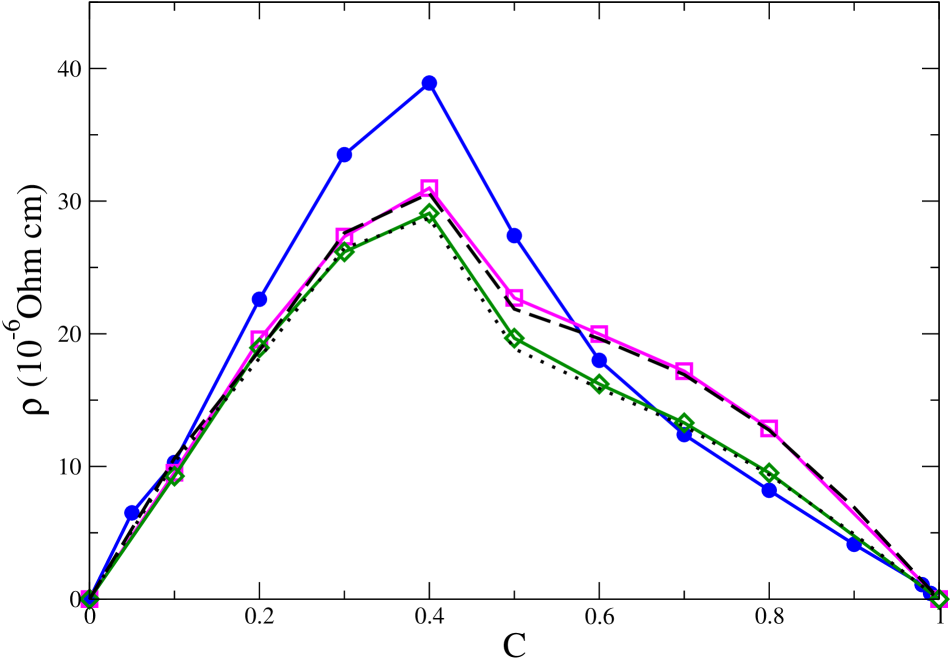
Figure 1: The resistivity of randomly disordered alloys $Ag_{c}Pd_{1-c}$ alloys as a function of concentration $c$. The full lines are the NLCPA results (pink (green) lines with squares(diamonds) show those without (with) vertex corrections). The dashed curves show the CPA results (long dashes (dots) - without (with) vertex corrections). The experimental results of Guenault Guenhault are shown for comparison (full blue lines with filled circles).

VIII The effects of SRO on resistivity.

Many properties of alloys such as resistivity are affected by short-range order. Indeed resistivity measurements are often used to monitor the changes in SRO which occur in annealing processes. If an alloy undergoes defect annealing after having been cold-worked there are significant changes in its physical properties owing to microstructural changes. For technical applications it is important to know what these changes are so that physical properties can be controlled. SRO plays an important role in this and resistivity measurements are used to follow its kinetics.Migschitz Our formalism is designed to help the interpretation of such measurements since it can describe the effects of short-range order on transport properties of alloys. It enables the calculation of the resistivity of a system to be made for a prescribed degree of SRO via the setting of the cluster configurational probabilities $P_{\gamma_{C}}$. Hence it can aid the extraction of SRO attributes from resistivity measurements.

Our first application is to the b.c.c. based series of disordered $Cu_{c}Zn_{1-c}$ alloys. We implement the NLCPA resistivity formalism using the smallest clusters and coarsest Brillouin zone tiling, i.e. $N_{C}=2$. This means correlations only between nearest neighbors can be described. We incorporate SRO according to the following 3 prescriptions for the 4 configurational weights, $P_{1}=P(CuCu)$, $P_{2}=P(CuZn)$, $P_{3}=P(ZnCu)$ and $P_{4}=P(ZnZn)$:

• No SRO, $P(CuCu)=c^{2}$, $P(CuZn)=P(ZnCu)=c(1-c)$, $P(ZnZn)=(1-c)^{2}$.

• Short-range order (minimising number of like nearest neighbors), for $c>0.5$, $P(CuCu)=(2c-1)$, $P(CuZn)=P(ZnCu)=(1-c)$, $P(ZnZn)=0$ and for $c<0.5$, $P(CuCu)=0$, $P(CuZn)=P(ZnCu)=c$, $P(ZnZn)=(1-2c)$.

• Short-range clustering (maximising number of like nearest neighbors), $P(CuCu)=c$, $P(CuZn)=P(ZnCu)=0$, $P(ZnZn)=(1-c)$.

Figure 2 summarises our findings. Vertex corrections are included and are shown to be large for these systems. This concurs with earlier results for the randomly disordered alloys which have low d-electron weight in electronic structure around the Fermi energy. In the absence of any short-range ordering, the results show approximate adherence to the expected Nordheim $c(1-c)$ behavior and the results both with and without vertex corrections are very close to the CPA results and experimental results Ho . Incorporating short-range order with extent only between nearest neighbors decreases the resistivity as expected for all concentrations. The resistivity now follows a rough $c(1-c)+\lambda c^{2}(1-c)^{2}$ dependence so that the greatest reduction occurs at the stoichiometric concentration of $c=0.5$. Conversely when short-ranged clustering is included the resistivity increases for all concentrations and the $c(1-c)$ behavior returns. Evidently current is enhanced on both types of atom when they are surrounded by unlike neighbours. These results are in good agreement with experimental measurements of the resistivity which show the resistivity to decrease significantly when the alloys are annealed so that short-ranged order is induced. Ho

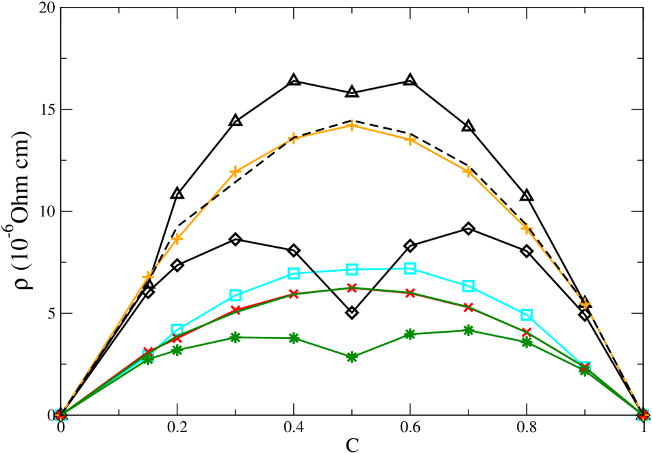
Figure 2: The resistivity of $Cu_{c}Zn_{1-c}$ alloys as a function of $c$, concentration. The full (red) line with crosses shows the calculations when no SRO is included.(These are nearly indistinguishable from the CPA results (green line)). The (green) line with asterisks shows the NLCPA results when SRO is included and the square boxes (light blue line) show results when short-ranged clustering is included. Results are also shown where the vertex corrections have not been included: full (yellow) line with plus signs - NLCPA results for no SRO, (the dashed line shows the CPA results); lines with diamonds - NLCPA results including SRO; and lines with triangles - NLCPA results including short-ranged clustering.

We have also investigated the effect of short-range order on $Ag_{c}Pd_{1-c}$ alloys by once more choosing configurational weights such that the number of like neighbours is minimised for each concentration. Figure 3 contains the results. The effect of SRO is less than that found in $CuZn$. Below $c=0.3$ the effect is negligible whereas for larger concentrations short-range order depresses the resistivity a little showing how the current is enhanced on a site when surrounded by unlike neighbors. Experimental measurements on $Ag_{c}Pd_{1-c}$ alloys find that annealing has a smaller effect Guenhault ; Swihart than in $Cu_{c}Zn_{1-c}$ in line with our calculations. It is also found that cold work causes little change to the resistivity suggesting that additional defects such as dislocations may already be present affecting the measurements. This may indicate the origin of our underestimate of the resistivity shown in Figure 1 and Figure 3.

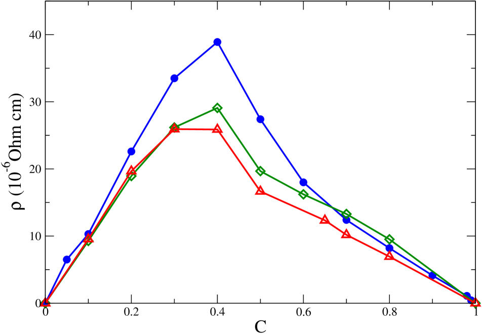
Figure 3: The resistivity of $Ag_{c}Pd_{1-c}$ alloys as a function of $c$, concentration. The full (green) line with diamonds shows the calculations when no SRO is included. The (red) line with triangles shows those when SRO is included. Vertex corrections are included in both plots. The experimental data Guenhault are also shown (blue line with filled circles).

IX Conclusions

Short-range ordering and clustering dramatically affect the transport properties of many alloys. Indeed resistivity measurements, which can be made easily and rapidly, provide a good way to monitor microstructural changes that occur in materials processing. In this paper we have described a way to make quantitative calculations of the resistivity of disordered systems which possess short-range order or clustering. The ab-initio theory starts from the density functional theory for these systems devised recently by Rowlands et al. derwyn dft using the SCF-KKR-NLCPA electronic structure method. Our first calculations for $Cu_{c}Zn_{1-c}$ and $Ag_{c}Pd_{1-c}$ show the expected decrease of resistivity when short-range order is imposed whereas short-ranged clustering produces an increase. For the randomly disordered alloys the results are very similar to those that have been produced from established KKR-CPA resistivity calculations based on Butler et al. work  butler4 ; butler1 . These first calculations have not included the effects of the short range order on the self-consistent charge densities and potentials that are available from the SCF-KKR-NLCPA method. So far also short-range clustering and ordering effects over only the shortest nearest atomic neighbor range have been included. The computational development work is in progress to remove these current practical limitations. The counterintuitive behavior of the resistivities of the K-state alloys such as $NiCr$,$NiMo$ and $PdW$ will be ideal next systems to study.

X Acknowledgements

The authors are grateful to B. L. Györffy for very useful discussions. They also acknowledge financial assistance from the UK EPSRC and the SSP 1145 ”MODERN AND UNIVERSAL FIRST-PRINCIPLES METHODS FOR MANY-ELECTRON SYSTEMS IN CHEMISTRY AND PHYSICS” as well as the SFB 689 ”Spinphänomene in reduzierten Dimensionen” of the DFG. Computing facilities for this work were provided by the University of Warwick Centre for Scientific Computing and the Universität München.

References

• (1) P. Soven, Phys. Rev. 156, 809 (1967).
• (2) P. Hohenberg and W. Kohn, Phys. Rev. 136, B864, (1964).
• (3) W. Kohn and L. J. Sham, Phys. Rev. 140, A1133 (1965).
• (4) D. D. Johnson, D. M. Nicholson, F. J. Pinski, G. M. Stocks and B. L. Gyorffy, Phys. Rev. Lett. 56, 2088 (1986).
• (5) D. D. Johnson, D. M. Nicholson, F. J. Pinski, G. M. Stocks and B. L. Gyorffy, Phys. Rev. B 41, 9701, (1990).
• (6) B. L. Györffy, Phys. Rev. B. 5, 2382 (1972).
• (7) G. M. Stocks, W. M. Temmerman, and B. L. Györffy, Phys. Rev. Lett. 41, 339 (1978).
• (8) B. L. Györffy, D. D. Johnson, F. J. Pinski, D. M. Nicholson, and G. M. Stocks in proceedings of the NATO Advanced Study Institute on Alloy Phase Stability, edited by G. M. Stocks and A. Gonis (Kluwer, Dordrecht, 1987), p. 421.
• (9) J. B. Staunton and B. L. Györffy, Phys. Rev. Lett. 69, 371 (1992).
• (10) M. Lüders, A. Ernst, M. Dane, Z. Szotek, A. Svane, D. Kodderitzsch, W. Hergert, B. L. Györffy and W. M. Temmerman, Phys. Rev. B 71, 205109 (2005).
• (11) J. S. Faulkner, Prog. Mat. Sci. 27, 1 (1982).
• (12) B. L. Györffy, B. Ginatempo, D. D. Johnson, D. M. Nicholson, F. J. Pinski, J. B. Staunton, and H. Winter, Philos. Trans. R. Soc. London, Ser. A 334, 515 (1991).
• (13) I.D.Hughes et al., Nature, 446, 650, (2007).
• (14) J. B. Staunton et al., Phys. Rev. Lett. 93, 257204, (2004).
• (15) G. M. Stocks and W. H. Butler, Phys. Rev. Lett. 48, 55 (1982).
• (16) W. H. Butler and G. M. Stocks, Phys. Rev. B 29, 4217 (1984).
• (17) W. H. Butler, Phys. Rev. B 29, 4224 (1984).
• (18) B. Velicky, Phys. Rev. B 184, 614 (1963).
• (19) R. Kubo, J. Phys. Soc. Jpn. 12, 570 (1957).
• (20) D. A. Greenwood, Proc. Phys. Soc. London 71, 585 (1958).
• (21) W. H. Butler, Phys. Rev. B 31, 3260 (1985).
• (22) J. C. Swihart, W. H. Butler, G. M. Stocks, D. M. Nicholson and R. C. Ward, Phys. Rev. Lett. 57, 1181 (1986).
• (23) J. Banhart, R. Bernstein, J. Voitländer and P. Weinberger, Solid State Commun. 77, 107 (1991).
• (24) J. Banhart, H. Ebert, P. Weinberger and J. Voitländer, Phys. Rev. B 50, 2104 (1994).
• (25) A. Gonis, Green Functions for Ordered and Disordered Systems, Studies in Mathematical Physics Vol. 4 (North-Holland, Amsterdam, 1992).
• (26) H. Thomas, Z. Phys. 129, 219 (1951).
• (27) A. Mookerjee and R. Prasad, Phys. Rev. B 48, 17724 (1993).
• (28) T. Saha, I. Dasgupta, and A. Mookerjee, Phys. Rev. B 50, 13267 (1994).
• (29) T. Saha, I. Dasgupta, and A. Mookerjee, J. Phys. Cond. Matt. 8, 1979 (1996).
• (30) J. Kudrnovsky and V. Drchal, Phys. Rev. B 41, 7515 (1990).
• (31) A. Mookerjee, J. Phys. C: Solid State Phys. 6, 1340 (1973).
• (32) L. J. Kaplan and T. Gray, Phys. Rev. B 14, 3462 (1976).
• (33) R. Haydock, V. Heine, and M. Kelly, J. Phys. C: Solid State Phys. 5, 2845 (1972).
• (34) K.K. Saha, A. Mookerjee and O. Jepsen, Phys. Rev. B 71, 094207 (2005).
• (35) K. Tarafder, A. Chakrabarti, K. K. Saha,2 and A. Mookerjee, Phys. Rev. B 74, 144204, (2006).
• (36) D. A. Rowlands, J. B. Staunton and B. L. Györffy, Phys. Rev. B 67, 115109 (2003).
• (37) D. A. Rowlands, J. B. Staunton, B. L. Györffy, E. Bruno and B. Ginatempo, cond-mat/0411347 (2005); D. A. Rowlands, J. B. Staunton, B. L. Györffy, E. Bruno and B. Ginatempo, Phys. Rev. B 72, 045101 (2005).
• (38) D. A. Rowlands, A. Ernst, B. L. Györffy and J. B. Staunton, Phys. Rev. B 73 165122 (2006).
• (39) D. A. Biava, S. Ghosh, D. D. Johnson, W. A. Shelton, and A. V. Smirnov, Phys. Rev. B 72, 113105 (2005).
• (40) S. Ghosh, D. A. Biava, W. A. Shelton, Physical Review B 73 085106 (2006).
• (41) D. Ködderitzsch, H. Ebert, D. A. Rowlands and A. Ernst, New J. of Phys. 9, 81, (2007).
• (42) M. Jarrell and H. Krishnamurthy, Phys. Rev. B 63, 125102 (2000).
• (43) M. H. Hettler, A. N. Tahvildar-Zadeh, M. Jarrell, Th. Pruschke and H. R. Krishnamurthy, Phys. Rev. B 58, 7475 (1998).
• (44) M. H. Hettler, M. Mukherjee, M. Jarrell, and H. R. Krishnamurthy, Phys. Rev. B. 61, 12739 (2000).
• (45) Th. Maier, M. Jarrell, Th. Pruschke, and J. Keller, Eur. Phys. J. B 13, 613 (2000).
• (46) M. Tsukada, J. Phys. Soc. Jpn. 32, 1475 (1972).
• (47) P. R. Tulip, J. B. Staunton, D. A. Rowlands, B. L. Györffy, E. Bruno and B. Ginatempo, Phys. Rev. B 73, 205109 (2006).
• (48) G. M. Batt and D. A. Rowlands, J. Phys.: Cond. Matt. 18, 11031 (2006).
• (49) E.Runge et al., Phys.Rev.Lett. 52, 997, (1984); E.K.U.Gross et al., Phys.Rev.Lett. 55, 2850, (1985); E.K.U.Gross et al. in ‘Density Functional Theory’, ed. R.F.Nalewajski, Springer Series ‘Topics in current Chemistry’ (1996).
• (50) W. G. Henry and P. A. Schroeder, Can. J. Phys. 41, 1076 (1963).
• (51) J. S. Faulkner and G. M. Stocks, Phys. Rev. B 21, 3222 (1980).
• (52) M. Hwang, A. Gonis, and A. J. Freeman, Phys. Rev. B 35, 8985 (1987).
• (53) H.Ebert in‘Electronic Structure and Physical Properties of Solids’, 535 of ‘Lecture Notes in Physics’ ed.;H.Dreysse (Springer, Berlin, 2000) and references therein; ‘The Munich SPRKKR band structure program package’ (2005); http://olymp.cup.uni-muenchen.de/ak/ebert/SPRKKR.
• (54) L. Nordheim, Ann.Phys. 9, 664, (1931).
• (55) J. Banhart and H. Ebert, Sol.Stat.Comm. 94, 445, (1995).
• (56) I. Turek, J. Kudrnovsky, V. Drchal and P.Weinberger, J. Phys.: Condensed Matter 16, 5607, (2004).
• (57) J. Banhart, Phil. Mag. B 77, 105, (1998).
• (58) A. M. Guenhault, Phil. Mag., 30, 641, (1974).
• (59) M.Migschitz et al., Acta.Mat. 44, 2831, (1996).
• (60) C. Y. Ho, Journal of Physical and Chemical Reference Data 12 : 183-322, (1983).