Thermal shifts and intermittent linear response of aging systems

Abstract

At time $t$ after an initial quench, an aging system responds to a perturbation turned on at time $t_{\rm w}<t$ in a way mainly depending on the number of intermittent energy fluctuations, so-called quakes, which fall within the observation interval $(t_{\rm w},t]$ [Sibani et al. Phys. Rev. B, 74, 224407 and Eur. J. of Physics B, 58,483-491, 2007]. The temporal distribution of the quakes implies a functional dependence of the average response on the ratio $t/t_{\rm w}$. Further insight is obtained imposing small temperature steps, so-called $T$-shifts. The average response as a function of $t/t_{\rm w,eff}$, where $t_{\rm w,eff}$ is the effective age, is similar to the response of a system aged isothermally at the final temperature. Using an Ising model with plaquette interactions, the applicability of analytic formulae for the average isothermal magnetization is confirmed. The $T$-shifted aging behavior of the model is described using effective ages. Large positive shifts nearly reset the effective age. Negative $T$-shifts offer a more detailed probe of the dynamics . Assuming the marginal stability of the ‘current’ attractor against thermal noise fluctuations, the scaling form $t_{\rm w,eff}=t_{\rm w}^{x}$, and the dependence of the exponent $x$ on the aging temperatures before and after the shift are theoretically available. The predicted form of $x$ has no adjustable parameters. Both the algebraic scaling of the effective age and the form of the exponent agree with the data. The simulations thus confirm the crucial rôle of marginal stability in glassy relaxation.

I Introduction

Rejuvenation, memory and other intriguing aspects of out-of-equilibrium thermal relaxation, a process widely known as aging, continue to attract experimental and theoretical interest  Lundgren86 ; Schultze91 ; Sibani91 ; Hoffmann97 ; Jonason98 ; Komori99 ; Komori00a ; Komori00b ; Normand00 ; Utz00 ; Bouchaud01 ; Nicodemi01 ; Bonn02 ; Berthier02 ; Takayama02 ; Jensen02 ; Sibani04a .

One starting point for theoretical analyses is the real space morphology of spin-glasses with short-range interactions, where thermalized domains form, with a linear size growing in time as $R(t)\propto t^{\lambda}$  Rieger93 ; Komori99 ; Komori00a ; Komori00b . The domain size corresponds to the thermal correlation length and can be extracted from numerical simulation data. Furthermore, the temperature dependence of the exponent $\lambda$ can be rationalized by assuming that the energy barrier controlling domain growth increases logarithmically in time Komori00b ; Rieger93 . The same logarithmic time dependence characterizes hierarchical models, which account for e.g. memory effects using configuration space, or ’landscape’ properties as starting point Vincent91 ; Hoffmann97 ; Dupuis02 . A third theoretical approach focuses on the relationship between linear response and autocorrelation functions. Numerical Andersson92 ; Sibani07 and experimental Svedlindh89 ; Herisson02 ; Buisson03 results show that the Fluctuation Dissipation Theorem (FDT) is applicable for observation times $t_{\rm obs}<t_{\rm w}$, where $t_{\rm w}$ is the time at which the perturbation is applied. While the FDT is broken for larger $t_{\rm obs}$, the proportionality between conjugate response and correlation functions may be restored asymptotically for large $t_{\rm w}$ and $t_{\rm obs}$, whence a general description flows in terms of effective temperatures Cugliandolo97 ; Castillo03 ; Buisson03 ; Calabrese05 . Last but not least, fluctuation spectra Crisanti04 ; Sibani05 ; Sibani06a ; Sibani06b ; Sibani07 ; Christiansen07 indicate that thermally activated aging processes, linear response functions included, are controlled by intermittent transitions between meta-stable attractors which irreversibly release the excess energy trapped in the initial configuration. These events, dubbed quakes, have statistical properties suggesting that they might be triggered by thermal fluctuations of record magnitude Sibani93a ; Sibani93 .

Based on the idea that metastable attractors of glassy systems are marginally stable, and that the transitions between them are hence induced by record sized thermal fluctuations, a ‘record dynamics’ scenario Sibani03 provides approximate analytical formulae for several physical quantities. The derivations ignore quasi-equilibrium properties, but are sufficiently general to support the universal character of off-equilibrium aging phenomena  Cipelletti00 ; Josserand00 ; Hannemann05 ; Anderson04 ; Oliveira05 ; Sibani93 ; Rieger93 . To buttress a comprehensive description of non-equilibrium aging based on record dynamics, this paper discusses numerical simulations of an Ising model with plaquette interactions, which has a glassy dynamical regime at low temperatures. The work extends numerical investigations Sibani06b ; Christiansen07 of the same model, and experimental and numerical studies of linear response in spin-glasses Sibani06a ; Sibani07 .

Aging under isothermal conditions is considered first, and analytic formulae for the average magnetization Sibani06a ; Sibani07 are verified. Secondly, the effect of ‘$T$-steps’ or ‘$T$-shifts’, small temperature steps of either sign applied concurrently with the magnetic field is analyzed in terms of effective ages. Replacing the age $t_{\rm w}$ as a scaling parameter, the effective age makes the response look similar to the isothermal response at the final temperature. Effective ages give an excellent parameterization of the average response for negative shifts, and a reasonable one for positive shifts. Fluctuation spectra cannot be fully described by an effective age.

For negative T-shifts, an algebraic relation between effective and true age exists Sibani04a , and the analytical dependence of the corresponding exponent on the temperatures before and after the step has no adjustable parameters. Both the algebraic scaling and the for of the exponent are confirmed by the simulations. The final discussion emphasizes the ramified connections of the present approach to other descriptions of aging dynamics.

 

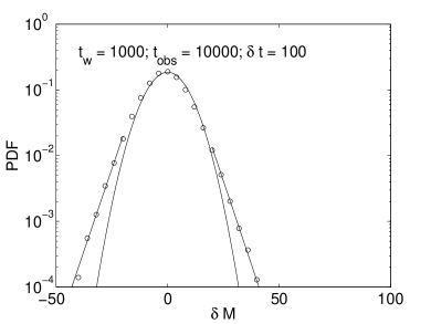
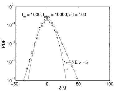
Figure 1: (color on line) (a): The PDF of the spontaneous magnetic fluctuations has a Gaussian central part and two symmetric intermittent wings. Data are sampled in the interval $t_{\rm w},t_{\rm w}+t_{\rm obs}$. (b): The same quantity (outer graph) when a field $H=0.3$ is turned on at $t_{\rm w}=1000$. The left intermittent wing is clearly reduced, and the right intermittent wing is amplified. The inner, almost Gaussian shaped, PDF is the conditional PDF obtained by excluding the magnetic fluctuations which happen in unison with the quakes. The lines are fits to a zero centered Gaussian and to two exponentials, which are obtained using different subsets of the data.

II Model and method

In spite of its simplicity and, in particular, in spite of its lack of quenched disorder and the triviality of its ground states, the p-spin model has full fledged aging behaviorLipowski00 ; Swift00 ; Sibani06b . In the model, $N$ Ising spins, $\sigma_{i}=\pm 1$ are placed on a cubic lattice with periodic boundary conditions. They interact through the plaquette Hamiltonian

$${\cal H}=-\sum_{{\cal P}_{ijkl}}\sigma_{i}\sigma_{j}\sigma_{k}\sigma_{l}+H\eta(t_{\rm w}-t)\sum_{i}\sigma_{i},$$ (1)

where first sum runs over all the elementary plaquettes of the lattice, including for each the product of the four spins located at its corners. The second sum describes the coupling of the total magnetization $\sum\sigma_{i}$ to an external magnetic field. As expressed by the Heaviside step function $\eta(t_{\rm w}-t)$, the field jumps at $t=t_{\rm w}$ from zero to $H$.

The simulations utilize the Waiting Time Algorithm (WTM) Dall01 , a rejectionless algorithm endowed with an ‘intrinsic’ time unit approximately corresponding to one Monte Carlo sweep. By choosing a high energy random configuration as initial state for low temperature isothermal runs, an instantaneous thermal quench is effectively achieved. All simulations temperatures are within the model aging regime, $0.5<T<2.5$. To improve the statistics, PDF data are collected over $2000$ independent runs for each set of physical parameters. Other statistical data are collected over $1000$ independent runs.

In the following, the symbol $t$ stands for the time elapsed from the initial quench (and from the beginning of the simulations). The field is switched on at time $t_{\rm w}$, and $t_{\rm obs}=t-t_{\rm w}$ is the ‘observation’ time, during which data are collected. The external field jumps from zero to $H=0.3$ at $t=t_{\rm w}$. The thermal energy is denoted by $E$, the magnetization by $M$ and the fluctuations by $\delta E$ and $\delta M$ respectively. The latter are calculated as finite time differences over time intervals of length $\delta t\ll t_{\rm obs}$. The average magnetization per spin is denoted by $\mu_{\rm ZFCM}$.

III Results

That intermittent physical changes occurring in an aging process should be statistically subordinated to the quakes Oliveira05 ; Sibani06a ; Sibani07 ; Sibani06 is a crucial element of a record dynamics description. For completeness, we therefore include recent supporting evidence Christiansen07 related to the present model.

$\begin{array}[]{cc}\includegraphics[width=195.12767pt,height=173.44534pt]{mvsttwbt11.eps}&\includegraphics[width=195.12767pt,height=173.44534pt]{mvsttwbt13.eps}\\ \includegraphics[width=195.12767pt,height=173.44534pt]{mvsttwbt17.eps}&\includegraphics[width=195.12767pt,height=173.44534pt]{mvsttwbt19.eps}\end{array}$

Figure 2: (Color on line) For each temperature indicated, the four panels depict scaling plots of the average magnetization per spin, vertically adjusted by the constant $b(t_{\rm w})$. The values of $t$ range from $t=t_{\rm w}$ to $400t_{\rm w}$, with $t_{\rm w}=50,100,200,500$ and $1000$, (green, blue, magenta, black, and red circles respectively). The black line is a fit to Eq.(3).

The circles in Fig. (1) (see Ref. Christiansen07 ) show, on a logarithmic vertical scale, PDFs of the magnetic fluctuations $\delta M$ in the interval $[t_{\rm w},t_{\rm w}+t_{\rm obs}]$. The data in the left panel are spontaneous magnetic fluctuations (no field), while those in the right panel are effected by an external magnetic field switched on at $t=t_{\rm w}=1000$. In both panels, intermittent wings extend a zero-centered central Gaussian spectrum. The magnetic field enhances the positive wing, reduces the negative one, and leaves the Gaussian spectrum unchanged. In the right panel, a conditional PDF (stars) is also shown. The PDF is obtained by removing from the statistics all magnetic fluctuations occurring within the same or the next $\delta t$ as energy fluctuations of magnitude $\delta E\leq-5$. As the threshold chosen delimits the intermittent behavior of the heat flow PDF Christiansen07 , the filtering removes the magnetic fluctuations concurrent with the quakes. Since the resulting conditional PDF is nearly Gaussian, the intermittent magnetic fluctuations carrying the average magnetic response are all closely associated to the quakes. Furthermore, the energy, and, in particular, the quakes, are hardly affected by the magnetic field. Therefore, the quakes dissipate the excess energy entrapped in the initial (zero field) configuration Sibani06b ; Christiansen07 , and the field probes but does not modify the spontaneous intermittent dynamics.

As argued in ref. Sibani03 , the number of quakes in the interval $(t,t^{\prime})$ is theoretically described by a Poisson distribution with average

$$n_{I}(t^{\prime},t)=\alpha(N)\ln(t/t^{\prime}).$$ (2)

In the theory, $\alpha(N)$ depends linearly on the system size $N$ and not at all on temperature. The present model has nearly the same behavior Christiansen07 .

III.1 Isothermal aging

For physical processes subordinated to statistically independent quakes, the number, $n$, of quakes falling in a given observation interval assumes the rôle of the time variable in a homogeneous Markov process. The corresponding moments represent physical observables, and admit eigenvalue expansions. By averaging such expansions over the Poisson distribution of $n$, analytic formulas are obtained for the moments Sibani06 ; Sibani06a ; Sibani07 which depend on the ratio $t/t_{\rm w}$ between the end-points, $t_{\rm w}$ and $t$, of the observation interval. These expressions can usually be truncated after a few leading terms. E.g. the average linear response of the p-spin model is well approximated by

$$\mu_{\rm ZFCM}=b_{0}+a_{m}\ln(\frac{t}{t_{\rm w}})+b_{m}(\frac{t}{t_{\rm w}})^{\lambda_{m}},$$ (3)

where $b_{0}$, $a_{m}$, $b_{m}$ and $\lambda_{m}$ are parameters. The exponent $\lambda_{m}$ is negative, whence, asymptotically, the behavior becomes logarithmic. Figure (2) shows the average linear response versus $t/t_{\rm w}$ for the temperatures indicated in the four plots. Each plot displays data sets (dots) for $t_{\rm w}=100,200,400,600,800,1000$ and $2000$. The full line is a fit to Eq. (3). In order to include the stationary contribution to the magnetization, which is ignored in the theory, the constant $b_{0}$ in Eq.(3) is modified by an additive $t_{\rm w}$ dependent term. The correction increases with $t_{\rm w}$, but stays within a few percent of the total. The black line is obtained by fitting to Eq. (3). For the smallest values of the abscissa, the quality of the data collapse, and consequently, of the fit, is higher the higher the temperature. For larger values of the abscissa, all fits are equally satisfactory. In summary, the isothermal aging behavior is rather well described by Eq. (3).

III.2 The effect of T-shifts

The response function of spin-glasses Granberg88 ; Komori00b is systematically affected by a small temperature change, a so called $T$-shift, applied during the aging process, usually together with a field switch at age $t_{\rm w}$. E.g. the logarithmic derivative $S(t_{\rm w},t_{\rm obs})$ of the average magnetization as a function of $t_{\rm obs}$ peaks at $t_{\rm obs}=t_{\rm w}$ under isothermal conditions, and the peak moves to a lower, respectively higher, value when positive, respectively negative, temperature shifts are applied. As the same effect can be achieved isothermally at the final temperature using a shorter, respectively longer $t_{\rm w}$, an effective age $t_{w,{\rm eff}}$ expectedly provides a natural and general parameterization. A study of the intermittent heat transfer of the E-A spin glass model Sibani04a under a $T$-shift, and the present study, confirm and to some extent qualify this conclusion.

$\begin{array}[]{cc}\includegraphics[width=195.12767pt,height=173.44534pt]{19to15tw100.eps}&\includegraphics[width=195.12767pt,height=173.44534pt]{19to15tw1000.eps}\\ \includegraphics[width=195.12767pt,height=173.44534pt]{17to15tw100.eps}&\includegraphics[width=195.12767pt,height=173.44534pt]{17to15tw1000.eps}\end{array}$

Figure 3: (Color on line) For the temperatures indicated, the four panels depict scaling plots of the average magnetization per spin, shifted by the constant $b_{0}(t_{\rm w})$. In each panel, three sets of data are shown. The ordinate is the average linear response under different conditions. The abscissa is, a part from an additive constant, the system age $t$, scaled with either the true or the effective age. The two nearly overlapping data sets are for: i) Isothermal response at the indicated temperature, versus the age scaled by $t_{\rm w}$. ii) $T$-shifted response, plotted versus the system age scaled by $t_{w,{\rm eff}}$ . The quality of the collapse of these two data sets gauges the relevance of the effective age parameterization. iii) Same data as ii), but using the actual $t_{\rm w}$ value to scale the age.

Below, we consider how both negative and positive $T$-shifts affect the average response function of the plaquette model. We furthermore discuss how negative shifts affect the spectrum of intermittent magnetization fluctuations.

$\begin{array}[]{cc}\includegraphics[width=195.12767pt,height=173.44534pt]{upstep1.eps}&\includegraphics[width=195.12767pt,height=173.44534pt]{upstep2.eps}\\ \includegraphics[width=195.12767pt,height=173.44534pt]{upstep3.eps}&\includegraphics[width=195.12767pt,height=173.44534pt]{upstep4.eps}\end{array}$

Figure 4: (Color on line) The four panels depict, for the temperatures indicated, scaling plots of the average magnetization per spin, vertically adjusted by the constant $b_{0}(t_{\rm w})$. In each panel, three sets of data are shown. The ordinate is the average linear response under different conditions. The abscissa is, a part from an additive constant, the system age $t$, scaled with either the true or the effective age. The two nearly overlapping data sets are i) isothermal response at the given temperature, versus the age scaled by $t_{\rm w}$. ii) $T$ shifted response. The data are plotted versus the age scaled by $t_{w,{\rm eff}}$. The quality of the collapse of the first two data sets gauges the relevance of the effective age parameterization. iii) Same data as ii), but using the actual $t_{\rm w}$ value to scale the age.

Figure (3) shows the average magnetic response, vertically adjusted by a small $t_{\rm w}$ dependent term as previously discussed, for a negative $T$-shift imposed concurrently with the field switch at $t_{\rm w}$. Each panel of Fig. (3) contains three curves. In the lowest curve the $T$-shifted magnetization is plotted versus the scaling variable $t/t_{\rm w}-1$. The two, nearly overlapping, and higher lying, curves are i) the $T$-shifted data again, now plotted versus $t/t_{w,{\rm eff}}-1$, with $t_{\rm w,eff}$ chosen to maximize the data collapse. ii) Isothermal magnetization at the final temperature, plotted versus $t/t_{\rm w}-1$. Clearly, scaling by a suitable effective age accounts rather well for the average linear response following a negative $T$-shift.

$\begin{array}[]{cc}\includegraphics[width=390.25534pt,height=346.89731pt]{ScaledPDF.eps}\end{array}$

Figure 5: (Color on line) The PDF of magnetic fluctuations for isothermal (stars) and $T$-shifted (circles) protocols. The data are collected in intervals of type $[t,50t]$. The initial ages are $t_{\rm w,eff}=6400$ for isothermal aging and $t_{\rm w}=1000$ for $T$-shifted aging. The $\delta M$ values are calculated over intervals of size $\delta t=500$. A full collapse would imply the full equivalence of the $T$-shifted response and the isothermal response of a system of the correct effective age. The lines are fits to a zero centered Gaussian and to two exponentials, which are obtained using different subsets of the data.

Figure (4) is similar to Fig. (3), except that the applied $T$ shifts are now positive. In each panel, the highest lying curve shows the $T$-shifted magnetization versus $t/t_{\rm w}-1$. The two lower lying curves are i) the $T$ shifted magnetization data, now plotted versus $t/t_{\rm w,eff}-1$, and, ii) the magnetization curve obtained for isothermal aging at the final temperature, plotted versus $t/t_{\rm w}-1$. Note that the transient effects produced by a positive shift are not fully described by an effective age. Consequently, the ‘best’ value of $t_{\rm w,eff}$ is obtained by a fit which only maximizes data overlap for large $t/t_{\rm w}$ values.

Figure (4) shows that positive $T$ shifts lead, as expected, to effective ages smaller than the actual ages. The best achievable data collapse is not as good as for negative shifts, especially for small values of $t/t_{\rm w}$. Since a positive $T$-shift destroys, totally or in part, the current configuration, it apparently induces additional dynamical effects not well represented by an effective age. Qualitatively, the numerical results for positive shifts concur with a crucial hypothesis of record dynamics, namely that the attractors successively visited are all marginally stable, i.e. they are destabilized by a record sized thermal fluctuation. Increasing the temperature leads to larger thermal fluctuations, and hence to the destruction of the configuration reached at $t_{\rm w}$. Negative shifts have more subtle consequences, which yield to an analytical description. We first consider how negative shifts affect the spectrum of the magnetization fluctuations. Secondly, the algebraic relationship between true and effective age is explained theoretically and checked against simulation data.

A system undergoing a negative $T$-shift $T=1.9\rightarrow T=1.5$ at $t_{\rm w}=1000$ has, according to Fig. (3), second panel, an effective age $t_{\rm w,eff}\approx 6400$ . If its dynamics were fully equivalent to the isothermal dynamics of a system of age $t_{\rm w,eff}\approx 6400$, the PDFs of magnetization differences $\delta M$ calculated over intervals of the same length $\delta t$ would overlap in the two cases. In Fig. (5), the PDF of isothermal fluctuations for a system with $t_{\rm w}=6400$ (stars), are compared to the corresponding PDF of a $T$-shifted system of age $t_{\rm w}=1000$ (circles). Both data sets are plotted on a logarithmic vertical scale. The Gaussian parts overlap, but the intermittent tails do not. They are however parallel, meaning that the weight of the intermittent fluctuations relative to the weight of the Gaussian fluctuations is higher in the $T$-shifted than in the isothermal case, even though the normalized size distribution of the intermittent fluctuations is the same in both cases. Since the Gaussian fluctuations have zero average, the average response is described via $t_{\rm w,eff}$ as previously discussed.

$\begin{array}[]{cc}\includegraphics[width=195.12767pt,height=173.44534pt]{tweff_vs_tw.eps}&\includegraphics[width=195.12767pt,height=173.44534pt]{an_tw_vs_tweff.eps}\end{array}$

Figure 6: (Color on line) The left panel shows the algebraic relationship between the effective and the actual age for the three different $T$-shifts $1.6\rightarrow 1.5$ (red squares), $1.8\rightarrow 1.5$ (green polygons) and $1.6\rightarrow 1.4$ (blue diamonds). Other cases analyzed are not shown for graphical reasons The full lines correspond to the analytical prediction $t_{\rm w,eff}=t_{\rm w}^{x}$, where $x$ is determined by a least square fit. In the right panel, $t_{\rm w}^{x}$ is plotted versus $t_{\rm w,eff}$ using different symbols and colors for all available $x$ values. Deviations from the line gauge the discrepancy between predicted and observed behavior.

In a record dynamics scenario, the marginally stable attractor reached at $t_{\rm w}$ is associated to a dynamical barrier of magnitude $b(t_{\rm w})$, which matches the largest among the thermal fluctuations experienced by the system during the aging process. Thermal fluctuations are described by the equilibrium Boltzmann distribution $P(E)$ characterizing a single thermalized domain. In our case, the local density of states can be treated as a constant, and $P(E)\propto\exp(-E/T)$. The typical value of the largest among $t_{\rm w}$ fluctuations at temperature $T$ then scales as $b(t_{\rm w})\propto T\log(t_{\rm w})$ Sibani04a . Note that the Arrhenius escape time corresponding to $b(t_{\rm w})$ equals $t_{\rm w}$. . After a negative $T$-shift from $T_{i}$ to $T_{f}<T_{i}$, the Arrhenius time corresponding to the barrier $b(t_{\rm w})$ becomes $t_{\rm w,eff}=\exp(b(t_{\rm w})/T_{f})=t_{\rm w}^{T_{i}/T_{f}}$. We thus arrive at the conclusion that

$$t_{\rm w,eff}=t_{\rm w}^{x(T_{i},T_{f})};\quad x(T_{i},T_{f})=\frac{T_{i}}{T_{f}}.$$ (4)

Note that the temperature dependence of the exponent $x$ given by the above formula has no adjustable parameters. In Fig. (6), left panel, the empirically determined effective age is plotted versus the actual age on a log-log scale, for $T$-shifts $1.6\rightarrow 1.5$ (red squares) $1.8\rightarrow 1.5$ (green polygons) and $1.6\rightarrow 1.4$ (blue diamonds). The corresponding lines are obtained by linear regression, and their slopes provide a numerical estimate of the exponent $x$. Several other $T$-shifts are also considered, but the corresponding data are not shown for graphical reasons. The values of $t_{\rm w}^{x}$ corresponding to all available $x$ values are plotted versus the empirical effective age in the right panel of Fig. 6. The color and symbol coding is as follows: $1.6\rightarrow 1.5$ (green circles), $1.7\rightarrow 1.5$ (red squares), $1.8\rightarrow 1.5$ (blue diamonds) $1.9\rightarrow 1.5$ (black hexagons), $1.6\rightarrow 1.4$ (green polygons), $1.8\rightarrow 1.6$ (red stars), $1.8\rightarrow 1.6$ (blue plusses) and $2.0\rightarrow 1.8$, (black upper triangles). The full line is the theoretical prediction given in Eq. (4). Thus, the distance between the data points and the line represents the mismatch between data and theory. Except for shifts involving a relatively high initial temperature, especially for high values of the effective age, the agreement is good.

IV Discussion

Summarizing the results of Refs. Oliveira05 ; Sibani06 ; Sibani06a ; Sibani07 , using the number of quakes $n$ as an effective ‘time’ variable produces a translationally invariant re-parameterized aging description. This description relies on the statistical independence of the quakes and on the statistical subordination of physical changes to the quakes. It does not rely on the amount of change induces by the events. The (stochastic) changes may depend on the system type, on the observable considered, and even on $n$ itself. They can either be dealt with with further modeling assumptions Oliveira05 ; Sibani06 , or using the generic property that physical averages admit eigenvalue expansions, when treated as a function of $n$ Sibani06a . Averaging such expansions over the Poisson distribution of $n$ turns each exponential term e.g. $ae^{cn}$, into a fractional power $(t/t_{\rm w})^{\lambda_{c}}$, where the exponent $\lambda_{c}$ is related to the eigenvalue $c$ of the time re-parameterized problem by

$$\lambda_{c}(T)=\alpha(N)(e^{c(N,T)}-1).$$ (5)

The dependence of the exponent on the system size $N$ and temperature $T$ is now explicitely introduced. Note that the symbol $\lambda_{c}$ here denotes a generic exponent, and is not to be confused with the (nearly) homonymous dynamical exponent $\lambda$ widely used in the literature. Considering that $\alpha(N)\propto N$, several exponents may exist which diverge with $N$. These exponent are dynamically irrelevant as the corresponding modes quickly decay to zero. Some exponents may remain bounded in the thermodynamical limit, namely if the eigenvalue of the time-re-parameterized problem, $c(N)$ vanishes as $1/N$ or faster, as $N\rightarrow\infty$. Eigenvalues approaching zero faster than $1/N$ correspond to frozen modes, and are also dynamically irrelevant. Observable power-laws are thus connected to relaxation ‘time’ scales of the re-parameterized dynamics which diverge linearly with system size, see e.g. Ref. Sibani06 for an explicit demonstration of such linear divergence. The corresponding exponents have the form $\lambda_{c}(T)=\alpha(N)c(N,T)$, which is asymptotically independent of $N$ for large $N$.

Far away from equilibrium, and hence far from saturation, the smallest relevant exponent can be small enough to justify the further expansion $(t/t_{\rm w})^{\lambda_{c}}\propto 1+\lambda_{c}\ln(t/t_{\rm w})$ for a wide range of $t/t_{\rm w}$. If a logarithmic time dependence exists, it will be dominant for large values of $t/t_{\rm w}$. This is widely observed and implies that linear response and autocorrelation are again proportional. An effective temperature can then be defined, albeit in a non-universal manner Calabrese05 via the Fluctuation Dissipation ratio..

Numerical studies of domain growth convincingly show that the characteristic linear size of a thermalized domain increases algebraically in time Rieger93 ; Komori00b . In this context, the $T$ dependence of the growth exponent $\lambda$ indicates that the energy barrier surmounted at age $t$ grows logarithmically with $t$. The proposed explanation is however ad hoc and differs from the original assumptions of Fisher and Huse Fisher88 , who expected a power-law scaling. In record dynamics, the same logarithmic scaling flows from the proportionality between said barrier and the typical size of extremal thermal fluctuations at age $t$. This property leads directly to the temperature dependence of the exponent $x$ given in Eq. (4). Thus, even though the linear domain size $R(t)$ does not appear conspicuously in the present description, central aging features are clearly associated to properties of localized domains. Firstly, the presence of non-interacting domains can be deduced from the statistical properties of energy and linear response fluctuations Sibani05 ; Sibani06b ; Christiansen07 , e.g. it produces the linear system size dependence of the factor $\alpha$. Secondly, an approximately hierarchical energy landscape is required: In such landscape energy fluctuations of record size are, by construction, necessary to trigger any changes of metastable attractor. Last but not least, the temperature independence of $\alpha$”Sibani07 ; Christiansen07 is only possible if the landscape is invariant to a change of energy scale.

In conclusion, a record dynamics description accounts for: i) the linear response phenomenology of aging systems, including the effect of temperature shifts. ii) The origin of asymptotic descriptions in term of effective temperatures. iii) The interplay of real space properties, i.e. domains, and hierarchical properties associated to the energy landscape of each domain.

V Acknowledgments

Financial support from the Danish Natural Sciences Research Council is gratefully acknowledged. The authors are indebted to the Danish Center for Super Computing (DCSC) for computer time on the Horseshoe Cluster, where most of the simulations were carried out.

References

- [1] L. Lundgren, P. Nordblad, and L. Sandlund. Memory behaviour of the spin glass relaxation. Europhysics Letters, 1:529–534, 1986.
- [2] C. Schultze, K. H. Hoffmann, and P. Sibani. Aging phenomena in complex systems: A hierarchical model for temperature step experiments. Europhys. Lett., 15:361–366, 1991.
- [3] P. Sibani and K.H. Hoffmann. Relaxation in complex systems : local minima and their exponents. Europhys. Lett., 16:423–428, 1991.
- [4] S. Schubert K.H. Hoffmann and P. Sibani. Age reinitialization in spin-glass dynamics and in hierarchical relaxation models. Europhys. Lett., 38:613–618, 1997.
- [5] K. Jonason, E. Vincent, J. Hammann, J. P. Bouchaud, and P. Nordblad. Memory and Chaos Effects in Spin Glasses. Phys. Rev. Lett., 81:3243–3246, 1998.
- [6] T. Komori, H. Yoshino and H. Takayama. Numerical study on aging dynamics in the 3D Ising spin-glass model. I. Energy relaxation and domain coarsening. J. Phys. Soc. Japan, 68:3387–3393, 1999.
- [7] T. Komori, H. Yoshino and H. Takayama. Numerical study on aging dynamics in the 3D Ising spin-glass model. II. Quasi-equilibrium regime of spin autocorrelation function. J. Phys. Soc. Japan, 69:1192–1201, 2000.
- [8] T. Komori, H. Yoshino and H. Takayama. Numerical study on aging dynamics in Ising spin-glass models. Temperature change protocols . J. Phys. Soc. Japan, 69:228–237, 2000.
- [9] Valéry Normand, Stéphane Muller, Jean-Claude Ravey, and Alan Parker. Gelation kinetics of gelatin: A master curve and network modeling. Macromolecules, 33:1063–1071, 2000.
- [10] Marcel Utz, Pablo G. Debenedetti, and Frank H. Stillinger. Atomistic simulation of aging and rejuvenation in glasses. Phys. Rev. Lett., 84:1471–1474, 2000.
- [11] Jacques Hammann Jean-Philippe Bouchaud, Vincent Dupuis and Eric Vincent. Separation of time and length scales in spin glasses: Temperature as a microscope. Phys. Rev. B, 65:024439, 2001.
- [12] Mario Nicodemi and Henrik Jeldtoft Jensen. Aging and memory phenomena in magnetic and transport properties of vortex matter: a brief review. J. Phys A, 34:8425, 2001.
- [13] D.Bonn, S. Tanase, B. Abou, H. Tanaka and J. Meunier. Laponite: Aging and shear rejuvenation of a colloidal glass. Phys. Rev. Lett., 89:015701, 2002.
- [14] Ludovic Berthier and Jean-Philippe Bouchaud. Geometrical Aspects of Aging and Rejuvenation in the Ising Spin Glass: A Numerical Study. Phys. Rev. B, 66:054404, 2002.
- [15] Hajime Takayama and Koji Hukushima. Numerical Study on Aging Dynamics in 3D Ising Spin-Glass Model. III. Cumulative Memory and ‘Chaos’ Effects in the Temperature Shift Protocol. J. Phys. Soc. JPN, 71:3003–3010, 2002.
- [16] H. Jeldtoft Jensen and Mario Nicodemi. Memory effects in response functions of driven vortex matter. Europhys. Lett., 57:348, 2002.
- [17] Paolo Sibani and Henrik Jeldtoft Jensen. How a spin-glass remembers. memory and rejuvenation from intermittency data: an analysis of temperature shifts. JSTAT, page P10013, 2004.
- [18] H. Rieger. Non-equilibrium dynamics and aging in the three dimensional Ising spin-glass model. J. Phys. A, 26:L615–L621, 1993.
- [19] E. Vincent. Slow dynamics in spin glasses and other complex systems. In D. H. Ryan, editor, Recent progress in random magnets, pages 209–246. Mc Gill University, 1991.
- [20] V. Dupuis, E. Vincent, J.-P. Bouchaud, J. Hammann, A. Ito and H. Aruga Katori. Aging, rejuvenation and memory effects in Ising and Heisenberg spin glasses. Phys. Rev. B, 64:174204, 2002.
- [21] J-O. Andersson, J. Mattsson, and P. Svedlindh. Monte Carlo studies of Ising spin-glass systems: Aging behavior and crossover between equilibrium and nonequilibrium dynamics. Phys. Rev. B, 46:8297–8304, 1992.
- [22] P. Sibani. Linear response in aging glassy systems, intermittency and the Poisson statistics of record fluctuations. Eur. Phys. J. B, 58:483–491, 2007.
- [23] P. Svedlindh, K. Gunnarsson, P. Nordblad, L. Lundgren, H. Aruga and A. Ito. Equilibrium magnetic fluctuations of a short range ising spin glass. Phys. Rev. B, 40:7162–7166, 1989.
- [24] D. Hérisson and M. Ocio. Fluctuation-dissipation ratio of a spin glass in the aging regime. Phys. Rev. Lett., 88:257202, 2002.
- [25] L. Buisson, L. Bellon, and S. Ciliberto. Intermittency in aging. J. Phys. Condens. Matter., 15:S1163, 2003.
- [26] Leticia F. Cugliandolo, Jorge Kurchan, and Luca Peliti. Energy flow, partial equilibration, and effective temperature in systems with slow dynamics. Phys. Rev. E, 55:3898–3914, 1997.
- [27] Horacio E. Castillo, Claudio Chamon, Leticia F. Cugliandolo, José Luis Iguain and Malcom P. Kenneth. Spatially heterogeneous ages in glassy systems. Phys. Rev. B, 68:13442, 2003.
- [28] Pasquale Calabrese and Andrea Gambassi. Ageing properties of critical systems. J. Phys. A, 38:R133–R193, 2005.
- [29] P. Sibani and H. Jeldtoft Jensen. Intermittency, aging and extremal fluctuations. Europhys. Lett., 69:563–569, 2005.
- [30] Paolo Sibani, G.F. Rodriguez and G.G. Kenning. Intermittent quakes and record dynamics in the thermoremanent magnetization of a spin-glass. Phys. Rev. B, 74:224407, 2006.
- [31] Paolo Sibani. Aging and intermittency in a p-spin model. Phys. Rev. E, 74:031115, 2006.
- [32] S. Christiansen and P. Sibani. Linear response and spontaneous fluctuations of aging systems: the p-spin model. arXiv:0709.1085 [cond-mat.stat-mech], 2007.
- [33] A. Crisanti and F. Ritort. Intermittency of glassy relaxation and the emergence of a non-equilibrium spontaneous measure in the aging regime. Europhys. Lett., 66:253–259, 2004.
- [34] P. Sibani, C. Schön, P. Salamon, and J.-O. Andersson. Emergent hierarchical structures in complex system dynamics. Europhys. Lett., 22:479–485, 1993.
- [35] P. Sibani and Peter B. Littlewood. Slow Dynamics from Noise Adaptation. Phys. Rev. Lett., 71:1482–1485, 1993.
- [36] Paolo Sibani and Jesper Dall. Log-Poisson statistics and pure aging in glassy systems. Europhys. Lett., 64:8–14, 2003.
- [37] Luca Cipelletti, S. Manley, R. C. Ball, and D. A. Weitz. Universal aging features in the restructuring of fractal colloidal gels. Phys. Rev. Lett., 84:2275–2278, 2000.
- [38] Christophe Josserand, Alexei V. Tkachenko, Daniel M. Mueth, and Heinrich M. Jaeger. Memory effects in granular materials. Phys. Rev. Lett., 85:3632–3635, 2000.
- [39] A. Hannemann, J. C. Schön, M. Jansen, and P. Sibani. Non-equilibrium dynamics in amorphous Si3B3N7. J. Chem. Phys., B 109:11770–11776, 2005.
- [40] L.P. Oliveira, Henrik Jeldtoft Jensen, Mario Nicodemi and Paolo Sibani. Record dynamics and the observed temperature plateau in the magnetic creep rate of type ii superconductors. Phys. Rev. B, 71:104526, 2005.
- [41] Paul Anderson, Henrik Jeldtoft Jensen, L.P. Oliveira and Paolo Sibani. Evolution in complex systems. Complexity, 10:49–56, 2004.
- [42] A. Lipowski and D. Johnston. Cooling-rate effects in a model of glasses. Phys. Rev. E, 61:6375–6382, 2000.
- [43] Michael. R. Swift, Hemant Bokil, Rui D. M. Travasso and Alan J. Bray. Glassy behavior in a ferromagnetic p-spin model. Phys. Rev. B, 62:11494–11498, 2000.
- [44] Jesper Dall and Paolo Sibani. Faster Monte Carlo simulations at low temperatures. The waiting time method. Comp. Phys. Comm., 141:260–267, 2001.
- [45] Paolo Sibani. Mesoscopic fluctuations and intermittency in aging dynamics. Europhys. Lett., 73:69–75, 2006.
- [46] P. Granberg, L. Sandlund, P. Nordblad, P. Svedlindh, and L. Lundgren. Observation of a time-dependent spatial correlation length in a metallic spin glass. Phys. Rev. B, 38:7097–7100, 1988.
- [47] Daniel S. Fisher and David A. Huse. Equilibrium behavior of the spin-glass ordered phase. Phys. Rev. B, 38:386–410, 1988.