Quantum Elastic Net and the Traveling Salesman Problem

Abstract

Theory of computer calculations strongly depends on the nature of elements the computer is made of. Quantum interference allows to formulate the Shor factorization algorithm turned out to be more effective than any one written for classical computers. Similarly, quantum wave packet reduction allows to devise the Grover search algorithm which outperforms any classical one. In the present paper we argue that the quantum incoherent tunneling can be used for elaboration of new algorithms able to solve some NP-hard problems, such as the Traveling Salesman Problem, considered to be intractable in the classical theory of computer computations.

I Introduction

Quantum parallel computations strongly differ from parallel calculi on the usual computers in a sense they use the same physical processor for all parallel operations. For example, if one wants to solve some property recognition problem one can prepare an initial state in the form:

$$|v_{0}\rangle=\frac{1}{\sqrt{2}}\sum_{\vec{x}}|\vec{x},0\rangle,$$

where $\vec{x}$ describes a possible assignment to binary variables, $x_{i}$, of the problem, $\vec{x}=(x_{1},x_{2},...,x_{n}),$ $x_{i}=0;1$, and the last bit in the array $v_{0}$ is left to store a result of calculations, $f(\vec{x})$, which is also presented in the binary form:

$$f(\vec{x})=1,$$

if the set $(x_{1},x_{2},...,x_{n})$ has a required property, and

$$f(\vec{x})=0$$

otherwise. Calculations are performed during time $t$ when the quantum computer evolves under unitary evolution operator,

$$|v_{0}\rangle\rightarrow|v_{t}\rangle=U_{t}|v_{0}\rangle=\frac{1}{\sqrt{2}}\sum_{\vec{x}}|\vec{x},f(\vec{x})\rangle.$$ (1)

In that way the results of calculations for all possible assignments of the variables $x_{1},x_{2},...,x_{n}$ turn out to be simultaneously evaluated and recorded on the same physical equipment.

It is clear that this method of computation gives a great economy of computer’s time and memory. Unfortunately, the described straightforward strategy is hampered by the following essential reason. Quantum mechanics says that if you try now to read out the results of calculations, you will succeed in observing only one of them, corresponding to some particular assignment of $\vec{x}$, and all other results will be irrevocably lost. Furthermore, the typical state of affairs with hard combinatorial problems is that results of calculations for most of assignments of $\vec{x}$ are equal to $0$, and there are very few of them (and namely they are of interest!) which correspond to $f(\vec{x})=1$. According to quantum mechanics, for the vector $|v_{t}\rangle$ in form (1), any particular result of observation of $f(\vec{x})$ will occur with probability $P(\vec{x})=1/2^{n}$. It is definitely forbidden to pick out at will any particular result of calculations on the stage of reading out. You can amplify the contribution of a result you want to know in the total wave packet only on the stage of the dynamical evolution described, as in the above given example, by the unitary evolution operator $U_{t}$, or in the general case, by more general operator taking into account dissipation and/or measurement processes. In other case, the property recognition problem can not be efficiently resolved (is intractable) since the probability of observation of a necessary result is exponentially suppressed as $P\sim 2^{-n}$.

Actually, there is no difference between calculations by quantum computers and the stochastic (Monte Carlo) calculations by classical computers, if one does not use some distinctive features of quantum systems to increase the probability of the result you want to obtain. For example, the quantum interference was used by P. Shor to determine a period of unknown function in his famous factorization algorithm Shor . This application of quantum mechanics is similar to usage of the interference for determination of a period of a crystal by Bragg’s scattering method. The Grover search algorithm increases the probability of the desired event with the help of the quantum wave packet reduction Grover . For the above considered example of property recognition problem, it is necessary to obtain after dynamical evolution a wave packet at which the components with $f(\vec{x})=1$ are present with probabilities much bigger than the components with $f(\vec{x})=0$.

In this paper we give some plausible arguments in favor of possibility of application of the quantum incoherent tunneling for solving some NP-hard combinatorial problems.

II ANALOG VERSUS DIGITAL COMPUTATIONS

The main difference between analog and digital computers consists in a manner of representation of numbers in them. In digital computers, the digital (usually binary) encoding of numbers is used, e.g., the value of $x$ may be represented as $100101$. In analog computers, different physical values, such as electrical currents, angles of rotation of gear wheels, etc, are representatives of mathematical values. Because of this the digital computers are much more compact and their size, $L$, scales with the quantity, $n$, of bits used for representation of the numbers as $L\sim n.$ Enclosing such numbers in analog computers requires much more large physical storage device, $L\sim e^{n},$ and, therefore, corresponding resources, such as energy, forces etc necessary for operations with the numbers are also exponentially large in this case.

One more difference following also from the manner of number representation concerns the property of universality: digital computers are ordinarily universal, analog computers are designed for solving some special problems only. For each particular digital computer, universality should be proved, i.e. every arithmetic, logical, and other operations should be constructed of the basic operations with digits.

Usually merely computations that do not use resources that grow exponentially are of interest (so-called efficient computations). For them the Strong Church’s Thesis was formulated Vergis : Any finite analog computer can be simulated efficiently by a digital computer, in a sense that the time required by the digital computer to simulate the analog computer is bounded by a polynomial function of the resources used by the analog computer. This Thesis resulted from a great experience gained during elaboration of classical computers and has a clear sense: every classical physical process can be efficiently simulated with the help of the digital computers.

Due to a great progress in development of digital computer techniques, analog computers are used now extremely seldom. Nevertheless, they survived in a virtual form inside digital computers as analog algorithms and turned into powerful heuristic methods for solution of optimization problems. The analog algorithms inherited from their natural ancestors the correspondence of computational schemes to some real physical processes in nature. Thus, the steepest descent method is based on gradient equations often used for far-from-equilibrium physical system description Rabinovich . It is used to find local minima. Simulated annealing describes the opposite situation when a physical system is very close to the equilibrium state at each moment of its slow dynamical evolution. It is an example of analog algorithms for minimization of a function called energy which imitates the process of physical annealing known in practice of crystal growing. It is experimentally discovered and theoretically understood that molten matter, to be subjected to slowly cooling, transforms into a crystalline state corresponding to the minimum of its free energy. Simulated annealing was the only method (in addition, of course, to the honest looking over all variants) which gave hope to find the global minimum of combinatorial problems. However, rigorous consideration showed that in fact the global minimum can never be reached Azencott , because simulated annealing with cooling schedule

$$T_{1},\;T_{2},\;...,\;T_{n}\rightarrow 0,$$

requires an exponential computation time:

$$t_{n}\sim\exp(A/T_{n}),\qquad A=const.$$

Main computation time losses take place at the lowest temperature reached during calculations and the minimum becomes more and more inaccessible at each step of cooling. Even a very simple minimization problem corresponding to a biased double well energy function shown in Fig.1 requires the cooling schedule

$$T_{n}\sim D/\ln\;n$$

and an exponential computational time, $t\sim\exp n$, and, therefore, is intractable in the frame of this algorithm.

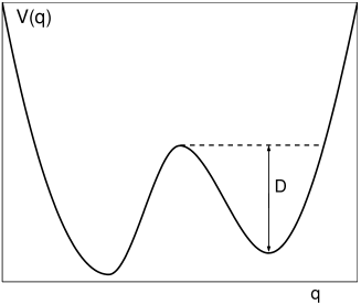
Figure 1: Minimization problem corresponding to a biased double well energy function requires the cooling schedule $T_{n}\sim D/\ln n$ and an exponential computational time in the frame of the simulated annealing algorithm.

Figure 2: Tunneling with dissipation allows particle to penetrate through the potential barrier in a finite space of time and then to stay at the point of the global minimum.

It appears at first sight, one can somehow accelerate cooling if does not require reaching the energy minimum on certainty. Then, after several reiteration, the position of the global minimum could be selected among all local minima found. But this strategy is, of course, wrong because no predictions about possibility to recognize the global minimum could be done if the true cooling schedule is broken.

Description of quantum systems often requires consideration of exponentially large number of different variants, e.g. a numerical realization of the path integral approach, and in particular for this purpose R. Feynman suggested quantum computers would be especially effective Feynman . For quantum computations no statements similar to the Strong Church’s Thesis were formulated so far and, therefore, both analog and digital approaches are still of equal interest. Below, we discuss an approaches to solution of the Traveling Salesman Problem by a quantum analog computing machine.

III INCOHERENT TUNNELING

In this section plausible reasoning are given in favor of incoherent tunneling as an effective remedy for solution of minimization problems on the stage of low temperatures when the simulated annealing algorithm is inoperative. To this goal let us consider again a biased double well potential shown in Fig.2 and a particle localized initially in the left local minimum at point $q_{0}$. Due to quantum tunneling effect, the particle can penetrate the potential barrier and fall into the global minimum at $q_{1}$. When the motion of the particle is accompanied by dissipation, there is a chance that the particle will stay at the global minimum and, hence, an optimization problem will be resolved.

A probable picture sketched above may be rigorously grounded. In the case when thermal energy, $k_{B}T$, is much less than energy, $\hbar\omega$, of classical oscillations at the positions of minima and the latter is, in its turn, much than the height of the potential barrier, $V_{bar}$, between the wells,

$$k_{B}T\ll\hbar\omega\ll V_{bar},$$

the process of tunneling with dissipation can be described on the base of multi-instanton calculations in the framework of the imaginary time functional integral approach Weiss . For temperature close to zero, the tunneling rate from $q_{0}$ to $q_{1}$ is given by an expression:

$$\gamma(q_{0}\rightarrow q_{1})=\frac{\pi}{2}\frac{\triangle^{2}}{\omega}\frac{1}{\Gamma(2\alpha)}\left(\frac{\sigma}{\omega}\right)^{2\alpha-1},$$

while the inverse transitions are suppressed,

$$\gamma(q_{1}\rightarrow q_{0})=0.$$

Here $\alpha=\eta d^{2}/2\pi\hbar$ is dimensionless damping coefficient, $d=q_{1}-q_{0}$ is the tunneling length, $\eta$ describes the force of friction, $F=-\eta dq/dt,$ and $\triangle$ is the tunnel matrix of undamped and unbiased system. The time of transition to the minimum, $\tau$, is finite now:

$$\tau\sim\frac{\hbar}{\gamma}.$$

Thus, at least for the double well, tunneling with dissipation, or incoherent tunneling, can be effectively applied for solving the minimization problem in the vicinity of zero temperatures.

Figure 3: Particle moves down the tilted periodic potential hill with a constant speed.

In the case of a tilted periodic potential, displayed in Fig.3, it is also possible to fulfil calculations explicitly and show that the time of transition from one local minimum to another is finite. An average position of the particle may be expressed as Weiss

$$\langle q(t)\rangle=v\;t,$$

where $v$ is mean drift velocity,

$$v=\frac{d\hbar}{\gamma}\;\tanh(\beta\hbar\sigma/2),\qquad\beta=1/k_{B}T.$$

Therefore, the time of minimization is proportional now to the sum of the tunneling time through all potential barriers on the way to the global minimum. It is naturally to suggest that a similar picture remains in the general case when the slope of the ”hill” is variable. Thus, the main question left to be discussed is how many local minima actually are on the way to the global minimum. In the case of the exponential number of them the problem would remain open.

The practice of solving optimization problems shows that usually there are much less of energy local minima than all possible (non minimal) values of energy. For example, number of local minima of the energy function was thoroughly investigated for the Hopfield Network Hopfield which was suggested as a mathematical model of the associative memory in human brain. Here each local minimum $H(\vec{x})$ is used to retain an information about $\vec{x}$ (called a pattern) since for a small deviation from $\vec{x}$, $\vec{x}\rightarrow\vec{x}+\vec{\delta x}$, the system returns back into $\vec{x}$ if it is navigated with the help of the gradient equations. It was shown that for random created patterns the number of local minima $M$ can be estimated as

$$M=0.138\;n,$$

where $n$ is a number of artificial neuron cells Hertz . Thus $M$ is only a linear function of the size, $n$, of the input. A similar result was obtained for an associative memory based on $Q$-state Potts-glass with biased patterns Bolle .

Further increase of the number of stored pattern up to $\alpha=1$ converts the Hopfield Network into a spin-glass Kinzel . The problem of finding the ground state in a spin-glass was studied in Barahona . This problem was shown to belong to the class of NP-hard problems both for three-dimensional case, and for two-dimensional lattice within a magnetic field. Infinite-ranged models of spin-glasses were considered in Kirkpatrick . Numerical experiments have shown the total number of local minima increases as some small power of $n$, rather than $\exp(n)$.

A drastic decrease of the number of local minima with different energies in the vicinity of the global one, for any system in the thermodynamic limit, follows also from the Nernst theorem for entropy,

$$\lim_{T\rightarrow 0}S(T)=0,$$

if there are no gaps of function $S(T)$ near $T=0$.

It is a commonly accepted method to demonstrate an efficiency of a new quantum algorithm with the help of a classical computer simulation of corresponding quantum calculations. But in our case there is no need to do so, because this has been already done. Actually, some kind of incoherent tunneling was used efficiently many times as an optimizing procedure during simulated annealing. For instance, in Kirkpatrick not only neighboring (in the Hamming sense) configuration of spin were checked during minimization, but also states which were 2, 3 and 4 steps away. When energy of a trial state was found to be less than energy of the current state the system was transmitted to the trial state. This corresponds to the under-barrier transitions through the potential barriers with 1, 2 and 3 Hamming’s steps of width. Of course, such a strategy is hampered for classical computers for more wider potentials barriers by a huge number of possible trial states. Quantum incoherent tunneling turns out to be much more effective because it allows to run over all local energy minima only, without examination of all possible values of energy for all possible trial states.

IV ELASTIC NET APPROACH TO THE TRAVELING SALESMAN PROBLEM AND ITS QUANTIZATION

The Traveling Salesman Problem (TSM-problem) is formulated as follows: given positions of cities, what is the shortest tour in which each city is visited once? It is evident that the total number of possible tours increases exponentially with the increase of number, $n$, of cities:

$$N_{tours}\sim e^{C\;n},$$

and their sequential consideration requires computing time which increases faster than any power of $n$. Therefore problem is considered as intractable in the classical theory of computation. In this section we show how the problem can be solved, at least in principle, using the quantum calculation technique. We consider the analog approach, because practical construction of quantum digital computers is still confronted with serious difficulties. Therefore, it is quite possible that quantum analog computers will win the digital ones, despite the opposite situation in the field of the classical computations.

Quantum analog computers for solving TSM-problem can be constructed on the base of the Elastic Net analog algorithm elaborated for the usual digital computers Durbin . The algorithm is grounded on a discrete form of the gradient equation,

$$\frac{d\vec{y}_{j}}{dt}=-\frac{\partial F}{\partial\vec{y}_{j}},$$

with free energy, $F$:

$$F=-\alpha k^{2}\sum_{i}\ln\sum_{j}e^{-|\vec{x}_{i}-\vec{y}_{j}|/2k^{2}}+\beta k\sum_{j}|\vec{y}_{j+1}-\vec{y}_{j}|^{2}.$$

For $\triangle t=1$ it is possible to write:

$$\triangle\vec{y}_{j}\simeq-\frac{\partial F}{\partial\vec{y}_{j}},\qquad\triangle F\simeq\sum_{j}\frac{\partial F}{\partial\vec{y}_{j}}\triangle\vec{y}_{j}\simeq-\sum_{j}\left(\frac{\partial F}{\partial\vec{y}_{j}}\right)^{2}<0.$$

This means that the algorithm directs the system to a local minimum of $F$ in accordance with the steepest descent method. The explicit form of $F$ was devised in Durbin using a very clear physical picture. Positions of cities are described by $\vec{x}_{i}$, points with coordinates $\vec{y}_{j}$ lie on an elastic string. Each point moves under the influence of two types of force. The first moves it towards those cities to which it is nearest; the second pulls it towards its neighbors on the string, acting to minimize the total string length.

The authors described an iteration procedure which consists in a gradual decrease of the value of a parameter $K$ describing a force and a range of interaction between $\vec{x}_{i}$ and $\vec{y}_{j}$ in such a way that at $K$ approaching to zero the range is transformed from a big value to very small one and the force is strongly increased. After applying this iteration procedure, an initial string in a form of a small circle placed nearby the cities’ centre of mass is converted into a salesman tour of a very high quality. Comparative analysis fulfilled in Peterson has shown that the performance of the Elastic Net algorithm is even of higher quality than that of Simulated Annealing. Therefore, one can use any of them, or some other described in Peterson , to find a preliminary solution to TSM-problem as an input for a further quantum computation.

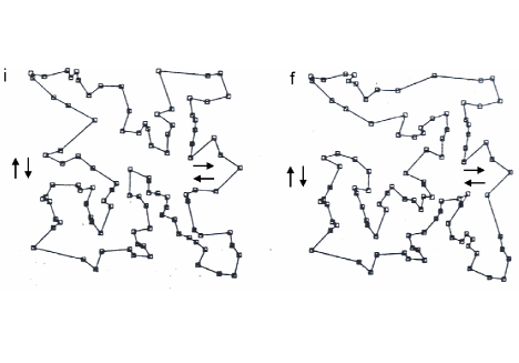
Figure 4: The process of solution of TSM-problem by the domain wall analog computer: an input, $i$, corresponding to a local minimum spontaneously decays into the final state, $f$, describing the global minimum.

Elastic string can be created as a physical computation device in the form of a mesoscopic domain wall in an antiferromagnetic thin film at low temperature. Tunneling of the domain walls in ferromagnetic and antiferromagnetic insulators through potential barriers (see, e.g., Chudnovsky ) is described in a similar way as incoherent tunneling of particles, considered in previous section. The role of the barriers can play defects or other singular points in the lattice. The domain wall has a variety of dissipative couplings to the magnons, photons, impurities, defects, and phonons. Nevertheless, it was shown that large domain walls, containing up to $10^{10}$ spins can behave as quantum objects at low temperatures Stamp . Both theory and experiment revealed a finite tunneling time of domain walls through potential barriers Chudnovsky . This gives an opportunity of devising an analog quantum computer using the incoherent tunneling effect. The process of solution of TSM-problem by this computer is shown schematically in Fig.4. Firstly, one creates an input, $i$, corresponding to some local minimum found with the help of the classical computer, and then, after a time, obtains a final state, $f$, as the solution. Points in the picture denote ”cities”, which are some kind of defects in the lattice that pin the domain wall to necessary locations. They may be some implanted atoms with high value of spins, or strongly magnetized atoms. Energy of the domain wall per unit of length (and, therefore, tension of the string) can be regulated by the material properties, or by a change of the mutual orientation of directions of spins on either side of the domain wall. It is clear that a value of tension should be small enough to prevent the string from a temptation to pass round some cities to minimize its length. Such a slack string limit corresponds to the strong shot-range interaction between the string and the cities considered as the last step of the iteration procedure in the classical Elastic Net analog algorithm Durbin . Therefore, quantum computer solution of the problem can be interpreted as a natural continuation of the classical algorithm after taking into account the tunneling processes. It is an easy task to examine that at least for a square lattice with the four nearest spin-spin interactions tension of the string is independent on its orientation. Thus, setting aside purely engineering problems, one may conclude that the Traveling Salesman Problem seems to be solvable by the quantum analog computer.

V ACKNOWLEDGMENT

The authors are thankful to Dr. M.V. Altaisky for useful remarks.

REFERENCES

- (1) Shor P. // Soc. Ind. Appl. Math. J. Comp. 1997. V.26. P.1484.
- (2) Grover L.K. // Proc. XXVIII Ann. ACM Symp. on the Theory of Computing (Philadelphia, Pennsylvania, 22-24 May 1996). P.212.
- (3) Vergis A., Steigilitz K., Dickinson B. // Mathematics and Computers in Simulation. 1986. V.28. P.91.
- (4) Rabinovich M.I., Ezersky A.B. Dynamic theory of pattern formation. // Janus-K, Moscow, 1998 (in Russian).
- (5) Feynman R. Intern. J. Theor. Phys. 1982. V.21. P.467.
- (6) Azencott R. // Sém. Bourbaki. No. 697. 1987-1988. P.223.
- (7) Weiss U., Grabert H. // Phys. Lett. A. 1985. V.108. P.63.
- (8) Hopfield J.J. // Proc. Nat. Acad. Sci. (USA). 1982. V.79. P.2554.
- (9) Hertz J., Krough A., Palmer R.G. Introduction to the theory of neural computation. // Addison-Wesley, Redwood City, CA, 1991.
- (10) Bolle D., Cools R., Dupont P. // J. Phys. A. 1993. V.26. P.549.
- (11) Kinzel W. // Z. Phys. B. 1985. V.60. P.205.
- (12) Barahona F. // J. Phys. A. 1982. V.15. P.3241.
- (13) Kirkpatrick S., Sherrington D. // Phys. Rev. B. 1978. V.17. P.4384.
- (14) Durbin R., Willshaw D. // Nature. 1987. V.326. P.689.
- (15) Peterson C. // Neural Computation. 1990. V.2. P.261.
- (16) Chudnovsky E. M. // J. Appl. Phys. 1993. V.73. P.6697.
- (17) Stamp P.C.E. // Phys. Rev. Lett. 1991. V.66. P.2802.