Intrinsic optical bistability of thin films of linear molecular aggregates: The two-exciton approximation

Abstract

We generalize our recent work on the optical bistability of thin films of molecular aggregates [J. Chem. Phys. 127, 164705 (2007)] by accounting for the optical transitions from the one-exciton manifold to the two-exciton manifold as well as the exciton-exciton annihilation of the two-exciton states via a high-lying molecular vibronic term. We also include the relaxation from the vibronic level back to both the one-exciton manifold and the ground state. By selecting the dominant optical transitions between the ground state, the one-exciton manifold, and the two-exciton manifold, we reduce the problem to four levels, enabling us to describe the nonlinear optical response of the film. The one- and two-exciton states are obtained by diagonalizing a Frenkel Hamiltonian with an uncorrelated on-site (diagonal) disorder. The optical dynamics is described by means of the density matrix equations coupled to the electromagnetic field in the film. We show that the one-to-two exciton transitions followed by a fast exciton-exciton annihilation promote the occurrence of bistability and reduce the switching intensity. We provide estimates of pertinent parameters for actual materials and conclude that the effect can be realized.

I Introduction

The phenomenon of optical bistability already has more than thirty years of history, going back to the theoretical prediction of McCall McCall74 in 1974, followed by experimental demonstration of the effect by Gibbs, McCall, and Venkatesan Gibbs76 in 1976 (see also Refs. Lugiato84, ; Gibbs85, , and Rosanov96, for an overview). Since then a vast amount of literature has been devoted to explore the topic (an extended bibliography can be found in our recent paper, Ref. Klugkist07a, ); controlling the flow of light by light itself is of great importance for optical technologies, especially on the micro- and nano-scale. More recently, new materials such as photonic crystals, Soljacic03 surface-plasmon polaritonic crystals, Wurtz06 and materials with a negative index of refraction, Litchinitser07 have revealed bistable behavior.

In our previous work, Klugkist07a we studied theoretically the bistable optical response of a thin film of linear molecular J-aggregates. To describe the optical response of a single aggregate, we exploited a Frenkel exciton model with an uncorrelated on-site energy disorder, taking into account only the optically dominant transitions from the ground state to the one-exciton manifold, while neglecting the one-to-two exciton transitions. Within this picture, an aggregate can be viewed as a meso-ensemble of two-level localization segments, Malyshev00 which allows for a description of the optical dynamics by means of a $2\times 2$-density matrix. Employing a joint probability distribution of the transition energy and the transition dipole moment of Frenkel excitons, allowed us to account for the correlated fluctuations of these two quantities, obtained from diagonalizing the Frenkel Hamiltonian with disorder. By solving the coupled Maxwell-Bloch equations, we calculated the phase diagram of possible stationary states of the film (stable, bistable) and the input-dependent switching time. From the analysis of the spectral distribution of the exciton population at the switching point, we realized that the field inside the film is sufficient to produce one-to-two exciton transitions, confirming a similar statement raised in Ref. Glaeske01, .

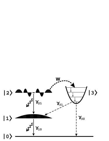
Figure 1: Four-level model of the film’s optical response. The input field induces transitions between the ground state $|0\rangle$, one-exciton manifold $|1\rangle$, and two-exciton manifold $|2\rangle$. The population of the latter is transferred with a rate $w$ to a vibronic molecular level $|3\rangle$, followed by fast relaxation between the vibronic sublevels towards the vibronic ground state. Finally, the latter undergoes relaxation to the one-exciton and/or ground state with the rates $\gamma_{31}$ and $\gamma_{30}$, respectively. The constants $\gamma_{10}$ and $\gamma_{21}$ denote the radiative decay of the one- and two-exciton states, respectively.

The goal of the present paper is to extend the one-exciton model Klugkist07a by including two-exciton states and transitions between the one- and two-exciton manifolds, respectively. Furthermore, two excitons spatially located within the same localization domain usually quickly annihilate, transferring their energy to an appropriate resonant monomer vibronic level. Stiel88 ; Sundstroem88 ; Minoshima94 ; Gaizauskas95 ; Scheblykin00a ; Shimizu01 ; Brueggemann03 ; Spitz06 Hence, the generalized model requires the consideration of exciton-exciton annihilation. Glaeske01 We will assume that exciton-exciton annihilation prevents the three-exciton states from playing a significant role in the response of the film. The relevant transitions of the model are depicted in Fig. 1.

To make the two-exciton model tractable, we will select the optically dominant transitions between the ground state and the one-exciton manifold (as we did in Ref. Klugkist07b, ), and also between the one- and two-exciton manifolds. Treating the different localization segments independently, in combination with the state selection, allows one to considerably reduce the set of relevant states, namely to four states of a segment: the ground state, the optically dominant one- and two-exciton states, and a high-lying molecular electronic or vibronic state, through which the excitons annihilate. This model has been implemented for the first time in Ref. Glaeske01, , using the simplifying assumption that the transition energies and transition dipole moments are correlated perfectly. Unlike Ref. Glaeske01, , we will account for the correct joint statistics of both quantities, similarly to our previous work. Klugkist07a The optical dynamics of a single localization segment is described within the framework of a $4\times 4$-density matrix. We derive a steady-state equation for the output field intensity as a function of the input intensity. The field inside the film is calculated taking into account the field produced by the aggregate dipoles. We find that, counterintuitively, tuning away from the resonance may, depending on the dephasing rate, promote bistable behavior. In addition, we show that fast exciton-exciton annihilation combined with slow relaxation from the high-lying vibronic level enhances the tendency towards bistablity. The phase diagram of bistability is computed and compared with the one-exciton model. We address also the realizability of the bistable behavior in actual materials.

The outline of this paper is as follows. In the next section we present our model of a single aggregate, consisting of a Frenkel Hamiltonian with uncorrelated on-site energy (diagonal) disorder (Sec. II.1). Next, we describe the selection of the optically dominant transitions in Sec. II.2 and introduce our model for the exciton-exciton annihilation of two-exciton states in Sec. II.3. In Sec. II.4, we formulate our approach, based on the density matrix equations in the $4\times 4$ space of states, as well as the Maxwell equation for a thin film of oriented linear J-aggregates. Section III deals with the results of our numerical analysis of the bistable optical response of the film in a multidimensional parameter space. We identify conditions that are most favorable for bistable behavior of the film. In Sec. IV, we estimate the driving parameters and the input light flux required for experimental realization of bistability for films of pseudoisocyanine J-aggregates. Section V summarizes the paper.

II Model

The geometry of the model system and the assumptions we adopt hereafter are essentially the same as in our previous paper. Klugkist07a In short, we aim to study the transmittivity of an assembly of linear J-aggregates arranged in a thin film (with the film thickness $L$ small compared to the emission wavelength $\lambda^{\prime}$ inside the film) and aligned in one direction, parallel to the film plane. The aggregates in the film are assumed to be decoupled from each other; their coupling to the environment is treated through phenomenological relaxation rates (see Ref. Klugkist07a, for a detailed discussion).

II.1 A single aggregate

We model a single aggregate as a linear chain of $N$ three-level monomers. The two lower states are assumed to form multi-exciton bands, as a result of strong dipole-dipole excitation transfer interactions between the monomers. To simplify the treatment of the multi-exciton states, we restrict ourselves to nearest-neighbor interactions. The transition dipole moments between the two lower molecular states are considered to align in one direction for all monomers. Then the (Frenkel) exciton part of the aggregate Hamiltonian reads

$$H_{0}=\sum_{n=1}^{N}\>\epsilon_{n}b_{n}^{\dagger}b_{n}-J\sum_{n=1}^{N-1}\left(b_{n}^{\dagger}b_{n+1}+b_{n+1}^{\dagger}b_{n}\right)\ ,$$ (1)

where $b_{n}^{\dagger}(b_{n})$ denotes the creation (annihilation) Pauli operator of an excitation at site $n$. The monomer excitation energies $\epsilon_{n}$ between the two lower states are modeled as uncorrelated Gaussian variables with mean $\epsilon_{0}$ and standard deviation $\sigma$. The parameter $J$ represents the magnitude of the nearest-neighbor transfer integral. We assume that it does not fluctuate. After applying the Jordan-Wigner transformation, the multi-exciton eigenstates are found as Slater determinants of one-exciton states $\varphi_{\nu n}$ with different $\nu$. Chesnut63 ; Juzeliunas88 ; Spano91 The multi-exciton eigenenergies are given by $\sum_{\nu=1}^{N}n_{\nu}\varepsilon_{\nu}$, with $\varepsilon_{\nu}$ being the one-exciton eigenenenrgies and $n_{\nu}=0,1$ depending on whether the $\nu$th state is occupied or not. Particularly, we will be interested in the one- and two-exciton states:

$$|\nu\rangle=\sum_{n=1}^{N}\varphi_{\nu n}|n\rangle\ ,$$ (2a)

$$|\nu_{1}\nu_{2}\rangle=\sum_{n_{1}>n_{2}}^{N}\left(\varphi_{\nu_{1}n_{1}}\varphi_{\nu_{2}n_{2}}-\varphi_{\nu_{1}n_{2}}\varphi_{\nu_{2}n_{1}}\right)|n_{1}n_{2}\rangle\ ,$$ (2b)

where $|n\rangle=b_{n}^{\dagger}|0\rangle$ and $|n_{1}n_{2}\rangle=b_{n_{1}}^{\dagger}b_{n_{2}}^{\dagger}|0\rangle$, and $|0\rangle$ is the ground state of the aggregate (with all monomers in the ground state). We also will need the transition dipole moments from the ground state $|0\rangle$ to a one-exciton state $|\nu\rangle$ and from a one-exciton state $|\nu\rangle$ to a two-exciton state $|\nu_{1}\nu_{2}\rangle$. In units of the single-molecule transition dipole moment, they obtain the dimensionless form

$$\mu_{\nu}=\sum_{n=1}^{N}\varphi_{\nu n}\ ,$$ (3a)

$$\mu_{\nu_{1}\nu_{2},\nu} =\sum_{n_{2}>n_{1}}\left(\varphi_{\nu n_{1}}-\varphi_{\nu n_{2}}\right)$$

$$\times\left(\varphi_{\nu_{1}n_{1}}\varphi_{\nu_{2}n_{2}}-\varphi_{\nu_{1}n_{2}}\varphi_{\nu_{2}n_{1}}\right)\ ,$$ (3b)

where it was assumed that the aggregate is small compared to an optical wavelength.

II.2 Selecting the dominant exciton transitions

At low temperatures, exciton states reduce their extension from the physical size of the aggregate to much smaller segments as a result of the disorder-induced Anderson localization Abrahams79 ; Schreiber82 . We will denote the typical size of these segments as $N^{*}$, often referred to as the number of coherently bound molecules or localization length in terms of the localization theory.

For J-aggregates, the optically dominant localized states reside in the neighborhood of the bottom of the exciton band. Some of them resemble $s$-like atomic states: they consist of mainly one peak with no node within the localization segment (see Fig. 2a). We will denote the subset of such states as ${\cal S}$. To find all the $s$-like states from the complete set of wave functions $\varphi_{\nu n}$, we used the rule proposed in Ref. Malyshev01, , $\big{|}\sum_{n}\varphi_{\nu n}|\varphi_{\nu n}|\big{|}\geq C_{0}$ with $C_{0}=0.75$. The inequality selects those states that contain approximately 75% of the density in the main peak. We found numerically that for a wide range of the disorder strength $\sigma$ ($0.05J<\sigma<J$), the thus selected states accumulate on average 73% of the total oscillator strength (equal to $N$). Recall that for a disorder-free aggregate, the optically dominant (lowest) exciton state contains 81% of the total oscillator strength of the one-exciton transitions (see, e.g., Refs. Fidder91, and Malyshev91, ). Furthermore, we have shown that the $s$-like states, used as a basis to calculate the linear absorption spectrum, well reproduce its peak position and the shape of its red part, failing slightly in describing the blue wing, where higher-energy exciton states contribute as well. Klugkist07b From this, we conclude that our procedure to select the optically dominant ($s$-like) one-exciton states works well.

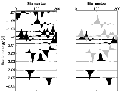
Figure 2: (a) The lowest 12 one-exciton states of a chain of length $N=500$ for a particular disorder realization at the disorder strength $\sigma=0.1J$. (b) A subset of $s$ states (black) and $p_{s}$ states (gray) that mostly contribute to the ground state to one-exciton and to the one-to-two exciton transitions. The average single molecule transition energy $\epsilon_{0}$ was chosen as origin of the energy scale.

Similar to the $s$-like states, one may also distinguish states that resemble atomic $p$ states. They have a well defined node within localization segments and occur in pairs with $s$-like states. Each pair forms an $sp$ doublet localized on the same chain segment. The levels within a doublet undergo quantum level repulsion, with their spacing nicely following the one that exists between $k=1$ and $k=2$ exciton states in a homogeneous chain of size $N^{*}$. Malyshev01 From the theory of multi-exciton transitions in homogeneous aggregates, Knoester93 we know that the Slater determinant of the $k=1$ and $k=2$ states forms the two-exciton state that predominantly contributes to the two-exciton optical response. This gives us a solid ground to believe that the $s$-like one-exciton states and the two-exciton states composed of $(sp)$ doublets dominate the one-to-two exciton transitions in disordered aggregates (see below).

Usually, well defined $(sp)$ doublets occur below the bare exciton band edge at the energy $-2J$. These doublets are responsible for a hidden level structure of the Lifshits tail. Malyshev95 For the $s$-like states located close to or above the bare band edge, it is already impossible to assign a $p$-like partner localized on the same segment: higher-energy states have more than one node and spread over segments of size larger than $N^{*}$ (see Fig. 2). To obtain all the states that give a major contribution to the one-to-two exciton transitions, the following procedure has been used. First, we selected all the $s$-like states, as described above. After that, we considered all the two-exciton states $|s\nu\rangle$ given by Eq. (2b) and calculated the corresponding transition dipole moments $\mu_{s\nu,s}$. From the whole set of $\mu_{s\nu,s}$, we took the largest ones denoted by $\mu_{sp_{s},s}$, were the substrict $s$ in $p_{s}$ indicates its relation with the state $|s\rangle$. This procedure catches all true $sp_{s}$ doublets and assigns a partner to solitary $s$-like states, which do not necessarily look like real $p$ states. In Fig. 2b, we depicted the final set of the doublets selected from the states in Fig. 2a according to the above procedure, which contribute mostly to the one- and two-exciton transitions.

The average ratio of the oscillator strength of the thus selected transitions $|s\rangle\to|sp_{s}\rangle$ and $|0\rangle\to|s\rangle$ turned out to be approximately 1.4. For a homogeneous chain, this ratio equals 1.57 (then $|s\rangle=|k=1\rangle$ and $|sp_{s}\rangle=|k_{1}=1,k_{2}=2\rangle$). The similarity of these numbers gives support to our selection procedure. Even stronger support is obtained from computing the pump-probe spectrum, using our state selection, and comparing the result to that of the exact calculations. Klugkist07b The comparison revealed that the model spectrum only deviates from the exact one in the blue wing of the induced absorption peak, similarly to the linear absorption spectra.

II.3 Exciton-exciton annihilation

As was already mentioned in the Introduction, two excitons created within the same localization segment efficiently annihilate (the intra-segment annihilation in terms of Refs. Malyshev99, and Ryzhov01, ). Thus, the authors of Ref. Minoshima94, studied experimentally the exciton dynamics in J-aggregates of pseudoisocyanine bromide (PIC-Br) at low temperature and found a 200 fs component in the two-exciton state decay. They attributed this to the annihilation of two-excitons located within the same chain segment of typical size of $N^{*}=20$. We adopt this mechanism for $|sp_{s}\rangle$ states described in the preceding section. Note that 200 fs is much shorter than all other population decay times. Other processes, such as radiative decay, occur at times of tens-to-hundreds of picoseconds.

Two excitons located on different localization segments can also annihilate (the inter-segment annihilation in terms of Refs. Ryzhov01, ). This process, however, is much slower as compared to the intra-segment channel; Ryzhov01 we neglect it. The thermally activated diffusion of excitons accelerates the annihilation of excitons created far away from each other. We consider this diffusion-limited exciton annihilation as irrelevant to our problem, because for bistability to occur we need the majority of $s$-like states to be saturated (also see Sec. IV).

It is usually assumed that the annihilation occurs via transferring the two-exciton energy to a resonant molecular vibronic level (see, e.g., Ref. Stiel88, ), which undergoes a fast vibration-assisted relaxation to the ground vibronic state. The population collected in this state relaxes further to the one-exciton state $|1\rangle$ of the segment or to the ground state $|0\rangle$ of the aggregate (cf. Fig 1). In this way, one or two excitations, respectively, are taken from the system. In summary, a four-level model, including the ground, one- and two-exciton states, and a molecular vibronic level through which the excitons annihilate, should be employed to describe the optical response of the film in the two-exciton approximation.

II.4 Truncated density-matrix-field equations

Within the four-level model introduced in the preceding sections, we describe the optical dynamics of a segment in terms of a $4\times 4$ density matrix $\rho_{\alpha\beta}$, where the indexes $\alpha$ and $\beta$ run from 0 to 3, where $|1\rangle\equiv|s\rangle$ and $|2\rangle\equiv|sp_{s}\rangle$. We neglect the off-diagonal matrix elements $\rho_{30},\rho_{31}$, and $\rho_{32}$, assuming a fast vibronic relaxation within the molecular level 3. Within the rotating wave approximation, the set of equations for the populations $\rho_{\alpha\alpha}$ and for the amplitudes of the relevant off-diagonal density matrix elements $R_{\alpha\beta},(\alpha\neq\beta)$ reads Glaeske01

$$\dot{\rho}_{00}=\frac{1}{4}\mu_{10}\left[\Omega R^{*}_{10}+\Omega^{*}R_{10}\right]+\gamma_{10}\rho_{11}+\gamma_{30}\rho_{33}\ ,$$ (4a)

$$\dot{\rho}_{11}=-\gamma_{10}\rho_{11}+\gamma_{21}\rho_{22}+\gamma_{31}\rho_{33}+\frac{1}{4}\mu_{21}\left(\Omega R^{*}_{21}-\Omega^{*}R_{21}\right)-\frac{1}{4}\mu_{10}\left(\Omega R^{*}_{10}-\Omega^{*}R_{10}\right)\ ,$$ (4b)

$$\dot{\rho}_{22}=-\left(\gamma_{21}+w\right)\rho_{22}-\frac{1}{4}\mu_{21}\left(\Omega R_{21}^{*}-\Omega^{*}R_{21}\right)\ ,$$ (4c)

$$\dot{\rho}_{33}=-\gamma_{3}\rho_{33}+w\rho_{22}\ ,$$ (4d)

$$\dot{R}_{10}=-\left(i\Delta_{10}+\Gamma_{10}\right)R_{10}-\mu_{10}\Omega\left(\rho_{00}-\rho_{11}\right)+\frac{1}{2}i\mu_{21}\Omega^{*}R_{20}\ ,$$ (4e)

$$\dot{R}_{21}=-\left(i\Delta_{21}+\Gamma_{21}+\frac{1}{2}w\right)R_{21}-\mu_{21}\Omega\left(\rho_{11}-\rho_{22}\right)-\frac{1}{2}i\mu_{10}\Omega^{*}R_{20}\ ,$$ (4f)

$$\dot{R}_{20}=-\left(i\Delta_{10}+i\Delta_{21}+\Gamma_{20}+\frac{1}{2}w\right)R_{20}+\frac{1}{2}i\mu_{21}\Omega R_{10}-\frac{1}{2}i\mu_{10}\Omega R_{21}\ .$$ (4g)

Here, $\gamma_{10}=\gamma_{0}|\mu_{10}|^{2}$ and $\gamma_{21}=\gamma_{0}|\mu_{21}|^{2}$ are the radiative relaxation rates of the one-exciton state $|1\rangle$ and the two-exciton state $|2\rangle$, respectively, with $\gamma_{0}$ denoting the monomer radiative rate, and $\mu_{10}$ and $\mu_{21}$ being the corresponding dimensionless transition dipole moments. Furthermore, $w$ is the annihilation constant of the two-exciton state $|2\rangle$ and $\gamma_{3}=\gamma_{30}+\gamma_{31}$ is the population relaxation rate of the vibronic state $|3\rangle$. The constants $\Gamma_{10}=\gamma_{10}/2+\Gamma$ and $\Gamma_{21}=\Gamma_{20}=\gamma_{21}/2+\Gamma$ stand for the dephasing rates of the corresponding transitions. They include a contribution from the population decay as well as a pure dephasing part $\Gamma$, which, for the sake of simplicity, we assume equal for all off-diagonal density matrix elements and not fluctuating. By $\Delta_{10}=\omega_{10}-\omega_{i}$ and $\Delta_{21}=\omega_{21}-\omega_{i}$ we denote the detuning between the exciton transition frequencies $\omega_{10}$ and $\omega_{21}$, and the frequency $\omega_{i}$ of the incoming field. It is worth to notice that Eqs. (4) automatically conserve the sum of level populations: $\rho_{00}+\rho_{11}+\rho_{22}+\rho_{33}=1$.

The quantity $\Omega=d_{0}E/\hbar$ in Eqs. (4) is the amplitude $E$ of the field inside the film in frequency units, where $d_{0}$ is the transition dipole moment of a monomer and $\hbar$ is the Planck constant. It obeys the following equation Glaeske01

$$\Omega=\Omega_{i}+\Gamma_{R}\>\frac{N_{s}}{N}\,\Big{\langle}\mu_{10}R_{10}+\mu_{21}R_{21}\Big{\rangle}\ ,$$ (5)

where $\Omega_{i}=d_{0}E_{i}/\hbar$ is the amplitude $E_{i}$ of the incoming field in frequency units, $N_{s}$ is the average number of $s$-like states in an aggregate, and $\Gamma_{R}=2\pi n_{0}{d_{0}}^{2}kL/\hbar$ is the superradiant constant, an important parameter of the model. Malyshev99 ; Glaeske01 ; Klugkist07a In this expression, $n_{0}$ is the number density of monomers in the film, $k$ is the field wave number, and $L$ is the film thickness. The angular brackets in Eq. (5) denote the average over disorder realizations.

The set of equations (4) forms the basis of our analysis of the effects of one-to-two exciton transitions, exciton-exciton annihilation from the two-exciton state, and relaxation of the annihilation level back to the one-exciton and ground states on the optical bistable response from an ultrathin film of J-aggregates. In the remainder of this paper, we will be interested in the dependence of the transmitted field intensity $|\Omega|^{2}$ on the input field intensity $|\Omega_{i}|^{2}$, following from Eqs. (4) and (5).

III Steady-state analysis

III.1 Bistability equation

To study the stationary states of the system, we first consider the steady-state regime of the film’s optical response and set the time derivatives in Eqs. (4) to zero. Furthermore, we will mostly focus on the limit of fast exciton-exciton annihilation, assuming the annihilation constant $w$ to be largest of all relaxation constants and also much larger than the magnitude of the field inside the film, $|\Omega|$. The reason for the latter assumption is based on the fact that below the switching threshold, the field magnitude $|\Omega|^{2}\sim(\gamma_{0}\sigma^{*})$, Klugkist07a where $\gamma_{0}$ and $\sigma^{*}$ are the radiative decay rate of a monomer and the half width at half maximum (HWHM) of the linear absorption spectrum, respectively. As $\gamma_{0}\ll\sigma^{*}$, the magnitude of the field is also much smaller than $\sigma^{*}$. Above the switching threshold, $|\Omega|$ becomes comparable to $\sigma^{*}$. Klugkist07a The typical HWHM of J-aggregates of PIC at low temperatures is on the order of a few tens of cm^-1, which in time units corresponds to one picosecond. On the other hand, the time scale of exciton-exciton annihilation is 200 femtoseconds (see Sec. II.3). This justifies our assumption $|\Omega|\ll w$ and allows us to neglect $R_{20}$ in steady-state Eqs. (4), because $|R_{20}|\sim|\Omega/(i\Delta_{21}+\Gamma_{20}+w/2)|$. Within this approximation, we are able to derive a closed steady-state equation for the $\Omega$-vs-$\Omega_{i}$ dependence, which reads

$$|\Omega_{i}|^{2}=\Bigg{\{}\left[1+\gamma_{R}\frac{N_{s}}{N}\bigg{\langle}\mu_{10}^{2}\frac{\Gamma_{10}}{\Gamma_{10}^{2}+\Delta_{10}^{2}}\left(\rho_{00}-\rho_{11}\right)+\mu_{21}^{2}\frac{\Gamma_{21}+w/2}{\left(\Gamma_{21}+w/2\right)^{2}+\Delta_{21}^{2}}\left(\rho_{11}-\rho_{22}\right)\bigg{\rangle}\right]^{2}$$

$$+\left[\gamma_{R}\frac{N_{s}}{N}\bigg{\langle}\mu_{10}^{2}\frac{\Delta_{10}}{\Gamma_{10}^{2}+\Delta_{10}^{2}}\left(\rho_{00}-\rho_{11}\right)+\mu_{21}^{2}\frac{\Delta_{21}+w/2}{\left(\Gamma_{21}+w/2\right)^{2}+\Delta_{21}^{2}}\left(\rho_{11}-\rho_{22}\right)\bigg{\rangle}\right]^{2}\Bigg{\}}|\Omega|^{2}\ .$$ (6)

The steady-state populations are given by Glaeske01

$$\rho_{00}-\rho_{11}=\frac{1+\left(1+w\gamma_{03}/\gamma_{10}\gamma_{3}\right)S_{21}}{1+2S_{10}+\left(1+w\gamma_{03}/\gamma_{10}\gamma_{3}\right)S_{21}+\left(3+w/\gamma_{3}\right)S_{10}S_{21}}\ ,$$ (7a)

$$\rho_{11}-\rho_{22}=\frac{S_{10}}{1+2S_{10}+\left(1+w\gamma_{03}/\gamma_{10}\gamma_{3}\right)S_{21}+\left(3+w/\gamma_{3}\right)S_{10}S_{21}}\ ,$$ (7b)

where

$$S_{10}=\frac{\mu_{10}^{2}|\Omega|^{2}}{2\gamma_{10}}\frac{\Gamma_{10}}{\Delta_{10}^{2}+\Gamma_{10}^{2}}\ ,$$ (8a)

$$S_{21}=\frac{\mu_{21}^{2}|\Omega|^{2}}{2\left(\gamma_{21}+w\right)}\frac{\Gamma_{21}+w/2}{\Delta_{21}^{2}+\left(\Gamma_{21}+w/2\right)^{2}}\ .$$ (8b)

The terms proportional to $\mu_{21}^{2}$ in Eq. (III.1) describe the effects of the two-exciton state, exciton-exciton annihilation, and relaxation from the vibronic level back to the one-exciton and ground states. Equation (III.1) reduces to the one-exciton model considered in our previous paper Klugkist07a by setting $\mu_{21}=0$. Similarly to the one exciton model, Eq. (III.1) contains a small factor $N_{s}/N$, absent in the earlier paper, Ref. Glaeske01, . This smallness, however, is compensated by the $N_{s}$-scaling of the average in Eq. (III.1): it is proportional to $\langle(\mu_{10}^{2}+\mu_{21}^{2})\rangle/N_{s}\approx 2N/N_{s}\gg 1$. Klugkist07a Thus, the actual numerical factor in Eq. (III.1) is approximately 2. We stress that, unlike previous work, Glaeske01 Eq. (III.1) properly accounts for the joint statistics of all transition energies and transition dipole moments.

It is worth to notice that the second term in the first square brackets in Eq. (III.1) represents the imaginary part of the nonlinear susceptibility, while the one in the second square brackets is its real part. Hence, we will will refer to these terms as to absorptive and dispersive, respectively, following the convention adapted in the standard theory of bistability of two-level systems in a cavity. Gibbs76

We numerically solved Eq. (III.1), looking for a range of parameters ($\Gamma_{R},\sigma^{*},\Gamma,\gamma_{31},\gamma_{30}$) where the output-input dependence becomes S-shaped, the precursor for bistability to occur. In all simulations, we used linear chains of $N=500$ sites and the radiative constant of a monomer $\gamma_{0}=2\times 10^{-5}J$ (typical for monomers of polymethine dyes). The exciton-exciton annihilation rate was set to $w=5000\gamma_{0}$, corresponding to an annihilation time of 200 fs. Minoshima94 The average single molecule transition energy $\epsilon_{0}$ was chosen as origin of the energy scale. 10000 localization segments were considered in disorder averaging.

Figure 3 shows the output intensity $I_{\mathrm{out}}=|\Omega|^{2}/(\gamma_{0}\sigma^{*})$ versus the input intensity $I_{\mathrm{in}}=|\Omega_{i}|^{2}/(\gamma_{0}\sigma^{*})$, varying the superradiant constant $\Gamma_{R}$ from small to large values to find the threshold for $\Gamma_{R}$ at which bistablity sets in. The relaxation constants $\gamma_{30}$ and $\gamma_{31}$ from the state $|3\rangle$ were taken to be equal to the radiative rate of a monomer, $\gamma_{0}$, which is the smallest one in the problem under study. The incoming field was tuned to the absorption maximum $\Delta_{10}^{(0)}=\epsilon_{0}-\omega_{i}-2.02J$, which naively speaking is expected to give the lowest threshold for bibtability (see a discussion of the detuning effects in Sec. III.3). The other parameters of the simulations are specified in the figure caption. As follows from Fig. 3, for the given set of parameters the bistability threshold is $\Gamma_{R}^{c}=7\sigma^{*}$.

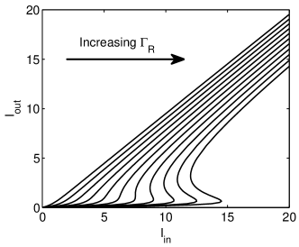
Figure 3: Examples of the output-input characteristics, demonstrating the occurrence of S-shaped behavior in the film’s optical response. Simulations were performed for a disorder strength $\sigma=0.1J$, resulting in an inhomogeneous HWHM $\sigma^{*}=0.024J$. The incoming field was tuned to the $J$-band maximum, $\Delta_{10}^{(0)}=\epsilon_{0}-\omega_{i}-2.02J$. The population relaxation rates of the vibronic state $|3\rangle$ were taken equal to the monomer decay rate, i.e., $\gamma_{31}=\gamma_{30}=\gamma_{0}$, while the dephasing constant $\Gamma=500\gamma_{0}$. In the plot, the superradiant constant $\Gamma_{R}$ ranges from $\sigma^{*}$ to $11\sigma^{*}$ in steps of $\sigma^{*}$ (left to right). The critical value for bistability to occur is seen to be $\Gamma_{R}^{c}=7\sigma^{*}$.

III.2 Effects of relaxation from the vibronic level

From the physical point of view, the most favorable conditions for bistability occur in the case of slow relaxation from the vibronic state $|3\rangle$, which is populated via a fast energy transfer from the two-exciton state $|2\rangle$ (fast exciton-exciton annihilation). Indeed, under these conditions, all population can be rapidly transferred to the state $|3\rangle$, and, accordingly, the system can be made transparent easier as compared to the case of the one-exciton model. Clearly, faster relaxation from the state $|3\rangle$ to the ground state $|0\rangle$ will deteriorate the condition for the occurrence of bistability, while slower relaxation improves the situation. Figure 4 demonstrates this.

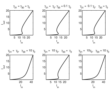
Figure 4: Examples of the output-input characteristics, demonstrating the effect of the relaxation rates $\gamma_{30}$ and $\gamma_{31}$ from the vibronic state $|3\rangle$ on the occurrence of bistability. The set of parameters used in the simulations are: $\sigma=0.1J$, $\Delta_{10}^{(0)}=\epsilon_{0}-\omega_{i}-2.02J$ (tuning to the J-band maximum), $\Gamma=500\gamma_{0}$, and $\Gamma_{R}=10\sigma^{*}$.

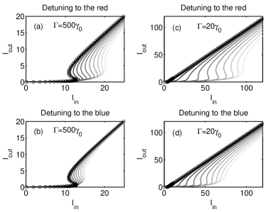
Figure 5: Examples of the output-input characteristics, demonstrating the combined effect of dephasing, $\Gamma$, and detuning off-resonance, $\Delta_{10}$, on the occurrence of bistability. In the simulations, the following set of parameters were used: a disorder strength $\sigma=0.1J$  (HWHM $\sigma^{*}=0.024J$), the exciton-exciton annihilation rate $w=5000\gamma_{0}$, the decay rates of the intermediate vibronic level $\gamma_{31}=\gamma_{30}=\gamma_{0}$, and the superradiant constant $\Gamma_{R}=10\sigma^{*}$. Panels (a) and (b) represent the results obtained for $\Gamma=500\gamma_{0}\sim\sigma^{*}$ when changing $\Delta_{10}$ from the absorption maximum at $\Delta_{10}^{(0)}=\epsilon_{0}-\omega_{1}-2.02J$ to the red (a) and to the blue (b) in 20 steps of $0.0025J$. The lighter curves correspond to a larger $\Delta_{10}$. Panels (c) and (d) show similar results obtained for $\Gamma=20\gamma_{0}\ll\sigma^{*}$.

III.3 Effects of detuning

As we mentioned in Sec. III.1, a naive viewpoint is that tuning of the incoming field to the absorption maximum is expected to give the lowest threshold for bistability. In this section, we show that in general this expectation is incorrect.

In Fig. 5 we plotted the results of our simulations of the film’s optical response as a function of the detuning off-resonance, $\Delta_{10}$, obtained for two values of the dephasing constant $\Gamma$. The disorder strength was set to $\sigma=0.1J$, resulting in an inhomogeneous HWHM $\sigma^{*}=0.024J$. From these data, one can distinguish two regimes. First, for a relatively large $\Gamma=500\gamma_{0}=0.02J\sim\sigma^{*}$ [panels (a) and (b)] the film’s response behaves according to the naive reasoning: the output-input characteristic looses its S-shaped form upon a deviation of the incoming field frequency from the absorption maximum. In contrast, as is observed in Figs. 5(c) and (d), for $\Gamma=20\gamma_{0}\ll\sigma^{*}$, when the absorption width is dominated by inhomogeneous broadening $\sigma^{*}$, tuning away from the resonance favors bistability.

We note that similar behavior has been found for assemblies of inhomogeneously broadened two-level emitters placed in a cavity, Gibbs76 ; Bonifacio78 ; Hassan78 where it was suggested that this counterintuitive frequency dependence results from the interplay of absorptive and dispersive contributions to the nonlinear susceptibility. We believe that our model exhibits the same spectral behavior because only the ground state to one-exciton transitions lead to spectral sensitivity. The one-to-two exciton transitions and the relaxation from the molecular vibronic level do not: the former because of the fast exciton annihilation, which washes out all spectral details, and the latter because it occurs from a relaxed state. Thus, all spectral features of the two-exciton model of the film’s bistability are driven by the ground state to one-exciton transitions. In other words, the one-exciton (two-level) model considered in our previous paper Klugkist07a is relevant for explaining the observed spectral behavior. In this case, the bistability equation (III.1) is reduced to

$$|\Omega_{i}|^{2}=\Bigg{\{}\left[1+\gamma_{R}\frac{N_{s}}{N}\bigg{\langle}\mu_{10}^{2}\frac{\Gamma_{10}}{\Gamma_{10}^{2}+\Delta_{10}^{2}+|\Omega|^{2}\Gamma_{10}/\gamma_{0}}\bigg{\rangle}\right]^{2}$$

$$+\left[\gamma_{R}\frac{N_{s}}{N}\bigg{\langle}\mu_{10}^{2}\frac{\Delta_{10}}{\Gamma_{10}^{2}+\Delta_{10}^{2}+|\Omega|^{2}\Gamma_{10}/\gamma_{0}}\bigg{\rangle}\right]^{2}\Bigg{\}}|\Omega|^{2}\ .$$ (9)

In our further analysis we show that, indeed, the interplay of the absorptive and dispersive terms in Eq. (III.3) is responsible for the counterintuitive spectral behavior. First, let us assume that we are far outside the resonance, i.e., $|\Delta_{10}|$ is large compared to the absorption HWHM, whether the homogeneous ($\Gamma^{*}=\langle\Gamma_{10}\rangle$) or the inhomogeneous one ($\sigma^{*}$). Then, the dispersive term drives the bistability, because its magnitude decreases as $|\Delta_{10}|^{-1}$ upon increasing $\Delta_{10}$, while the absorptive one drops faster, proportionally to $\Delta_{10}^{-2}$. The critical superradiant constant for the dispersive bistability has been reported to be $\Gamma_{R}^{c}=4\big{[}\Gamma^{*}+(\Gamma^{*2}+\Delta_{10}^{2})^{1/2}\big{]}$ (see, e.g., Ref. Gibbs76, ) which is reduced to $\Gamma_{R}^{c}\approx 4|\Delta_{10}|$ in the limit of $|\Delta_{10}|\gg\Gamma^{*}$. On the other hand, we found within the one-exciton model Klugkist07a that close to the resonance ($|\Delta_{10}|\ll\sigma^{*}$), where the contribution of the absorptive term is dominant, $\Gamma_{R}^{c}$ scales superlinearly with the HWHM, namely as $(\sigma^{*}/\Gamma^{*})^{\alpha}\Gamma^{*}$ with $\alpha\approx 1.7$. Similar scaling ($\Gamma_{R}^{c}=\sigma^{*2}/\Gamma^{*}$) has been obtained in Ref. Hassan78, for a collection of inhomogeneously broadened two-level systems placed in a cavity.

The superlinear dependence of $\Gamma_{R}^{c}$ for the absorptive type of bistability is a key ingredient in understanding the counterintuitive $\Delta_{10}$ behavior of the film’s optical response. Indeed, let $|\Delta_{10}|\gg\sigma^{*}$ and $\Gamma_{R}=4|\Delta_{10}|$, i.e., we are at the (dispersive) bistability threshold. Now, let us go back to the resonance, where bistability is of absorptive nature. Choose for the sake of simplicity $\Gamma_{R}^{c}=\sigma^{*2}/\Gamma^{*}$ as the critical value. If $4|\Delta_{10}|>\sigma^{*2}/\Gamma^{*}$, we are still above the (absorptive) bistability threshold, while in the opposite case bistable behavior is not possible. For $\sigma^{*}\sim\Gamma^{*}$, the line width is almost of homogeneous nature, and tuning away from the resonance deteriorates the conditions for the occurrence of bistability. Gibbs76 In our simulations, this holds for the case of $\Gamma=500\gamma_{0}=0.02J$ and $\sigma^{*}=0.024J$ [see panels (a) and (b) in Fig. 5].

To conclude this section, we note that the detuning effect found in our simulations is asymmetric with respect to the sign of $\Delta_{10}$: the behavior of $I_{\mathrm{out}}$ versus $I_{\mathrm{in}}$ is different for the incoming frequency tuned to the red or to the blue from the absorption maximum. We believe that this arises from the asymmetry of the absorption spectrum.

III.4 Phase diagram

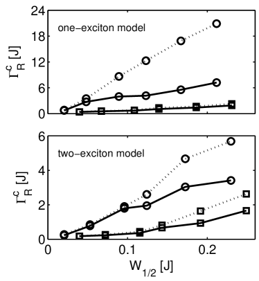
Figure 6: Phase diagram of the bistable optical response of a thin film in the ($\Gamma_{R},W_{1/2}$)-space, where $W_{1/2}=\sigma^{*}+\Gamma^{*}$, with $\Gamma^{*}=\Gamma+\langle\gamma_{10}\rangle/2$, is used as a measure for HWHM of the absorption spectrum accounting for contributions of inhomogeneous and homogeneous broadening (through $\sigma^{*}$ and $\Gamma^{*}$, respectively) to the total width of the $J$ band. The data were obtained by solving Eq. (III.1) for the input field tuned to the J-band center, $\Delta_{10}^{(0)}=\epsilon_{0}-\omega_{i}-2.02J$ and varying the disorder strength $\sigma$. In both panels, upper and lower curves correspond to $\Gamma=20\gamma_{0}$ and $\Gamma=500\gamma_{0}$, respectively. The open circles and squares represent the numerical data points, whereas the solid lines are a guide to the eye. The solid lines themselves represent the $W_{1/2}$-dependence of the critical superradiant constant $\Gamma_{R}^{c}$. Above (below) the curve for a given $\Gamma$, the film behaves in a bistable (stable) fashion. For comparison, we also plotted the phase diagram calculated under the assumption that the detuning is the only stochastic parameter (dotted curves, cf. Ref. Glaeske01, ).

In Fig. 6 we plotted the results of a comparative study of phase diagrams of the film’s response calculated within the one- and two-exciton model under the resonance condition, $\Delta_{10}^{(0)}=\epsilon_{0}-\omega_{i}-2.02J$. Presented is the critical superradiant constant $\Gamma_{R}^{c}$ versus the quantity $W_{1/2}=\sigma^{*}+\Gamma^{*}$, where $\Gamma^{*}=\Gamma+\langle\gamma_{10}\rangle/2$ is the homogeneous width of the one-exciton transition. The last term denotes the averaged rate of population relaxation from the one-exciton state to the ground state, see Eq. (4b). Roughly, $W_{1/2}$ can be interpreted as the HWHM of the absorption spectrum accounting for both inhomogeneous and homogeneous broadening (through $\sigma^{*}$ and $\Gamma^{*}$, respectively). The upper (lower) solid curve in both panels was obtained for the dephasing constant $\Gamma=20\gamma_{0}$ ($\Gamma=500\gamma_{0}$) and varying the disorder strength $\sigma$. For a given $\Gamma$, the film is bistable (stable) above (below) the corresponding curve. To compare these results with those calculated under the assumption that the detuning is the only stochastic parameter, Glaeske01 we also plotted the $\Gamma_{\mathrm{R}}^{c}$ vs $W_{1/2}$ dependence taking all the transition dipole moments and relaxation constants equal to their averaged values (dotted curves).

One of the principal conclusions which can be drawn from the data in Fig. 6 is that a more efficient dephasing helps the occurrence of bistability: all curves calculated for $\Gamma=20\gamma_{0}$ lie above those obtained for $\Gamma=500\gamma_{0}$. The physics of this behavior is simple: as the threshold for the absorptive bistability is $\Gamma_{R}^{c}=(\sigma/\Gamma^{*})^{\alpha}\Gamma^{*}$ (see Sec. III.3), a smaller $\Gamma^{*}$ gives rise to a higher threshold value for $\Gamma_{R}$. Thus, adjusting the dephasing constant $\Gamma^{*}$, we can manipulate the film’s optical response. This conclusion has been drawn already in Ref. Malyshev00, within the simplified one-exciton model.

Another observation is that the magnitude of the critical superradiant constant $\Gamma_{R}^{c}$ is considerably lower in the two-exciton model than in the one-exciton approach. This was to be expected from the physical reasoning which we presented above: a fast exciton-exciton annihilation combined with a slow relaxation from the high-lying molecular vibronic level favors bistability. Without showing detailed data, we note that also the critical switching intensity, i.e., the intensity calculated at the bistability threshold, is smaller in the two-exciton model compared to the one-exciton model. In both models, it also decreases upon increasing the dephasing rate.

Finally, from comparison between the solid and dotted curves in Fig. 6, it appears that, surprisingly, bistability is favored by the fact that also transition dipole moments and relaxation constants are stochastic variables and not only the detuning, as was assumed in the simplified model of Ref. Glaeske01, . At first glance this seems counterintuitive. However, inspection of changes in the absorption spectrum allows to shed light of on this result. We found that upon neglecting the fluctuations, the absorption spectrum, first, acquires a shift which introduces an additional detuning off-resonance. Second, the shape of the absorption spectrum gets more asymmetric. As the film’s response is sensitive to both the detuning and asymmetry, the combined effect of these changes produces the observed big difference between the two sets of calculations. In principle, this discrepancy may be reduced by adjusting the detuning; it is impossible, however, to correct for asymmetry. Most importantly, this comparison shows that to adequately calculate the film’s optical response, fluctuations of all variables should be taken into account.

IV Thin film of PIC: Estimates

In this section we will analyze low-temperature experimental data of $J$-aggregates of pseudo-isocyanine (PIC) to shed light on the feasibility of measuring optical bistability in a thin film of PIC. We will focus, in particular, on aggregates of PIC-Br studied experimentally in detail in Refs. Fidder90, ; Fidder93, and Minoshima94, . At low temperatures, the absorption spectrum of PIC-Br is dominated by a very narrow absorption band (HWHM = 17 cm^-1) peaked at $\lambda$ = 573 nm and red shifted relative to the main monomer feature ($\lambda$ = 523 nm). For these aggregates, vibration-induced intra-band relaxation is strongly suppressed (no visible Stokes shift of the fluorescence spectrum with respect to the $J$-band is observed). This favors a long exciton lifetime, which is highly desirable from the viewpoint of saturation, and thus for optical bistability. The lifetime of the exciton states forming the $J$-band in PIC-Br is conventionally assumed to be of radiative nature. For temperatures below about 40 K, it has been measured to be 70 ps. Fidder90

Within the one-exciton model studied in our previous paper, Klugkist07a we found that the number density of monomers, required for the driving parameter $\Gamma_{R}/\sigma^{*}$ to exceed the bistability threshold, has to obey $n_{0}>10^{19}$ cm^-3. Such densities can be achieved in thin films prepared by the spin-coating method. Misawa93 ; Ramunas Within the extended four-level model considered in the present paper, the critical ratio of $\Gamma_{R}/\sigma^{*}$ may be even lower. Thus, we believe that from the viewpoint of monomer density, J-aggregates of PIC are promising candidates.

Another important requirement for candidates, potentially suitable for bistable devices, is their photostability. J-aggregates are known to bleach if they are exposed for a long time to powerful irradiation. Therefore, it is useful to estimate the electromagnetic energy flux through the film. For the field slightly below the higher switching threshold, the dimensionless intensity inside the film obeys $I_{\mathrm{out}}=|\Omega|^{2}/(\gamma_{0}\sigma^{*})\approx 1$ (see, e.g., Fig.3). Using the expression for the monomer spontaneous emission rate $\gamma_{0}=32\pi^{3}d_{0}^{2}/(3\hbar\lambda^{3})$, we obtain $E_{\mathrm{out}}^{2}\approx 32\pi^{3}\hbar\sigma^{*}/(3\lambda^{3})$. The electromagnetic energy flux through the film is determined by the Poynting vector, whose magnitude is given by $S_{\mathrm{out}}=cE^{2}_{\mathrm{out}}/(4\pi)$. Being expressed in the number of photons $S_{\mathrm{out}}/(\hbar\omega_{10})$, passing per cm² and per second through the film, this value corresponds to $5\times 10^{21}$ photons/(cm² s). As is seen from Fig. 3, above the switching threshold the intensity inside the film rises by an order of magnitude. Hence, above threshold the electromagnetic energy flux reaches a value on the order of $S_{\mathrm{out}}\approx 5\times 10^{22}$ photons/(cm² s).

Furthermore, the typical time $\tau$ for the outgoing intensity $I_{\mathrm{out}}$ to reach its stationary value is on the order of the population relaxation time, which is 70 ps, except for values of $I_{\mathrm{out}}$ slightly above (below) the higher (lower) switching threshold, where the relaxation slows down. Klugkist07a This means that typically, a nanosecond pulse is enough to achieve the steady-state regime. Bearing in mind the above estimates for $S_{\mathrm{out}}$, we obtain the corresponding flux for a nanosecond pulse $S_{\mathrm{out}}\approx 10^{13}$ photons/(cm²  ns). On the other hand, for a thin film of thickness $L=\lambda/(2\pi)$ and number density of monomers $n_{0}=10^{20}$ cm^-3, the surface density is $n_{0}\lambda/(2\pi)\approx 10^{15}$ cm^-2. Combining these numbers, we conclude that only one photon per $20$ monomers produces the effect, which is well below the bleaching threshold. Ramunas

V Summary and concluding remarks

We theoretically studied the optical response of an ultrathin film of oriented J-aggregates with the goal to examine the effect of two-exciton states and exciton-exciton annihilation on the occurrence of bistable behavior. The standard Frenkel exciton model was used to describe a single aggregate: an open linear chain of monomers coupled by delocalizing dipole-dipole excitation transfer interactions, in combination with uncorrelated on-site disorder, which tends to localize the exciton states.

We considered a single aggregate as a meso-ensemble of exciton localization segments, ascribing to each segment a four-level system consisting of the ground state (all monomers in the ground state), an $s$-like one-exciton state, a two-exciton state constructed as the antisymmetric combination of this $s$-like state and an associated $p$-like one-exciton state, and a vibronic state of the monomer through which the two-exciton states annihilate. To select the $s$- and $p$-like states, a new procedure was employed which correctly accounts for the fluctuations and correlations of the transition energies and transition dipole moments, improving on earlier works. Glaeske01 The optical dynamics of the localization segment was described within the $4\times 4$-density matrix formalism, coupled to the total electromagnetic field. In the latter, in addition to the incoming field, we accounted for a part produced by the aggregate dipoles.

We derived a novel steady-state equation for the transmitted signal and demonstrated that three-valued solutions to this equation exist in a certain domain of the multi-parameter space. Analyzing this equation, we found that several conditions promote the occurrence of bistable behavior. In particular, a fast exciton-exciton annihilation, in combination with a slow relaxation from the monomer vibronic state, favors bistablity. In contrast, fast relaxation from the vibronic level to the ground state acts against the effect. Additionally, a faster dephasing also works in favor of the occurrence of bistability.

The interplay of detuning away from the resonance and dephasing was found to be counterintuitive. When homogeneous broadening of the exciton states (associated with the incoherent exciton-phonon scattering) is comparable with the inhomogeneous broadening (resulting from the localized nature of the exciton states), the detuning destroys bistability. Oppositely, at a slower dephasing, the bistability effect is favored by tuning away from the resonance. We relate this anomalous behavior to an interplay of the absorptive and dispersive parts of the nonlinear susceptibility, which jointly contribute to the overall effect.

We found that in general, including the one-to-two-exciton transitions promotes bistability. All critical parameters, such as the critical superradiant constant, driving the bistability, and the critical switching intensity are lower than in the one-exciton model. Klugkist07a In addition, bistable behavior is easier to reach if the ratio of the inhomogeneous and homogeneous width is reduced. We also found that the stochastic nature of the transition dipole moments (the aspect in which our model goes beyond Ref. Glaeske01, ) strongly influences the film’s optical response.

Estimates of parameters of our model for aggregates of polymethine dyes at low temperatures indicates that a film with a monomer number density on the order of $10^{20}$ cm^-1 and a thickness of $\lambda/2\pi$, achievable with the spin coating method, Misawa93 is sufficient to realize the effect. Under these conditions, one photon per 20 monomers produces the switching of the film’s transmittivity.

To conclude, we point out that a microcavity filled with molecular aggregates Lidzey98 ; Litinskaya04 ; Beltyugov04 ; Agranovich05 ; Zoubi05 in the strong coupling regime of excitons to cavity modes is another promising arrangement to realize an all-optical switch. The recent observation of optical bistability in planar inorganic microcavities Baas04 and the prediction of the effect for hybrid organic-inorganic microcavities Zoubi07 in the strong coupling regime suggest that organic microcavities can exhibit a similar behavior.

- (1) S. L. McCall, Phys. Rev. A 9, 1515 (1974).
- (2) H. M. Gibbs, S. L. McCall, and T. N. C. Venkatesan, Phys. Rev. Lett. 36, 1135 (1976).
- (3) L. A. Lugiato, in Progress in Optics, ed. E. Wolf (North-Holland, Amsterdam, 1984), vol. XXI, p. 71.
- (4) H. M. Gibbs, Optical Bistability: Controlling Light with Light (Academic, New York, 1985).
- (5) N. N. Rosanov, in Progress in Optics, ed. E. Wolf (North-Holland, Amsterdam, 1996), vol. XXXV, p. 1.
- (6) J. A. Klugkist, V. A. Malyshev, and J. Knoester, J. Chem. Phys. 127, 164705 (2007).
- (7) M. Soljacić, M Ibanescu, C. Luo, S. G. Jonson, S. Fan, Y. Fink, and J. D. Joannopoulos, Proceedings of SPIE, Photonic Crystal Materials and Devices, Ali Adibi, Alex Sherer, and Shawn Yu Lin, Editors, Vol. 5000, p. 200 (2003).
- (8) G. A. Wurtz, R. Polland, and A. V. Zayats, Phys. Rev. Lett. 97, 057402 (2006).
- (9) N. M. Litchinitser, I. R. Gabitov, A. I. Maimistov, and V. M. Shalaev, Opt. Lett. 32, 151 (2007).
- (10) V. A. Malyshev, H. Glaeske, and K.-H. Feller, Opt. Commun. 169, 177 (1999); J. Chem. Phys. 113, 1170 (2000).
- (11) H. Glaeske, V. A. Malyshev, and K.-H. Feller, J. Chem. Phys. 114 1966 (2001); Phys. Rev. A 114, 033821 (2002).
- (12) H. Stiel, S. Daehne, K. Teuchner, J. Lumin. 39, 351 (1988).
- (13) V. Sundström, T. Gillbro, R. A. Gadonas, A. Piskarskas, J. Chem. Phys. 89, 2754 (1988).
- (14) K. Minoshima, M. Taiji, K. Misawa, T. Kobayashi, Chem. Phys. Lett. 218, 67 (1994).
- (15) E. Gaizauskas, K.-H. Feller, and R. Gadonas, Opt. Commun. 118, 360 (1995).
- (16) I. G. Scheblykin, O. Y. Sliusarenko, L. P. Lepnev, A. G. Vitukhnovsky, M. Van der Auweraer, J. Phys. Chem. B 104, 10949 (2000); 105, 4636 (2001).
- (17) M. Shimizu, S. Suto, A. Yamamoto, T. Goto, A. Kasuya, A.Watanabe, M.Matsuda, Phys. Rev. B 64 (2001) 115417.
- (18) B. Brueggemann, V. May, J. Chem. Phys. 118, 746 (2003).
- (19) C. Spitz, S. Daehne, Int. J. Photoenergy 2006, 84950 (2006).
- (20) J. A. Klugkist, V. A. Malyshev, and J. Knoester, arXiv:0707.0826v1 [cond-mat.dis-nn]; J. Lumin., in print.
- (21) D. B. Chesnut and A. Suna, J. Chem. Phys. 39, 146 (1963).
- (22) G. Juzeliunas, Z. Phys. D 8, 379 (1988).
- (23) F. C. Spano, Phys. Rev. Lett. 67, 3424 (1991).
- (24) E. Abrahams, P. W. Anderson, D. C. Licciardello, and T. V. Ramakrishnan, Phys. Rev. Lett. 42, 673 (1979).
- (25) M. Schreiber and Y. Toyozawa, J. Phys. Soc. Jpn. 51, 1528 (1982); 51, 1537 (1982).
- (26) A. V. Malyshev and V. A. Malyshev, Phys. Rev. B 63 195111 (2001); J. Lumin. 94-95, 369 (2001).
- (27) H. Fidder, J. Knoester, and D.A. Wiersma, J. Chem. Phys. 95, 7880 (1991).
- (28) V. A. Malyshev Opt. Spektrosk. 71, 873 (1991) [Opt. Spectrosc. 71, 505 (1991)]; J. Lumin. 55, 225 (1993).
- (29) J. Knoester, Phys. Rev. A 47, 2083 (1993).
- (30) V. Malyshev and P. Moreno, Phys. Rev. B 51 14587 (1995); V. A. Malyshev and F. Dominguez-Adame, Am. J. Phys. 72, 226 (2004).
- (31) V. A. Malyshev, H. Glaeske, K.-H. Feller, Chem. Phys. Lett. 305, 117 (1999).
- (32) V. A. Malyshev, G. G. Kozlov, H. Glaeske, K.-H. Feller, Chem. Phys. 254, 31 (2000); I. V. Ryzhov and G. G. Kozlov and V. A. Malyshev, and J. Knoester, J. Chem. Phys. 114 5322 (2001).
- (33) R. Bonifacio and L. A. Lugiato, Lett. Nuovo Cimento 21, 517 (1978).
- (34) S. S. Hassan, P.D. Drummond, and D. F. Walls, Opt. Commun. 27, 480 (1978).
- (35) H. Fidder, J. Knoester, and D.A. Wiersma, Chem. Phys. Lett. 171, 529 (1990).
- (36) H. Fidder, J. Knoester, and D.A. Wiersma, J. Chem. Phys. 98, 6564 (1993).
- (37) K. Misawa, K. Minoshima, H. Ono, and T. Kobayashi, Appl. Phys. Lett. 63, 577 (1993).
- (38) R. Augulis, private communication.
- (39) D. G. Lidzey, D. D. C. Bradley, M. S. Skolnick, T. Virgili, S. Walker, and D. M. Whiteker, Nature 395, 53 (1998); D. G. Lidzey, D. D. C. Bradley, T. Virgili, A. Armitage, M. S. Skolnick, and S. Walker, Phys. Rev. Lett. 82, 3316 (1999).
- (40) M. Litinskaya, P. Reineker, and V. M. Agranovich, Phys. Stat. Sol. (a) 201, 646 (2004).
- (41) V. N. Bel’tyugov, A. I. Plekhanov, and V. V. Shelkovnikov, J. Opt. Technol. 71, 411 (2004).
- (42) V. M. Agranovich and G.C. La Rocca, Sol. St. Commun. 135, 544 (2005).
- (43) H. Zoubi and G. C. La Rocca, Phys. Rev. B 71, 235316 (2005).
- (44) D. G. Lidzey, in ”Thin Films and Nanostructures”, eds. V. M. Agranovich and F. Bassani (Elsevier, New York, 2003), Vol. 31, Chapt. 8.
- (45) A. Baas, J. Ph. Karr, H. Eleuch, and E. Giacobino, Phys. Rev. A 69, 023809 (2004).
- (46) H. Zoubi and G. C. La Rocca, Phys. Rev. B 76, 035325 (2007).