Robustly estimating the flow direction of information in complex physical systems

Abstract

We propose a new measure to estimate the direction of information flux in multivariate time series from complex systems. This measure, based on the slope of the phase spectrum (Phase Slope Index) has invariance properties that are important for applications in real physical or biological systems: (a) it is strictly insensitive to mixtures of arbitrary independent sources, (b) it gives meaningful results even if the phase spectrum is not linear, and (c) it properly weights contributions from different frequencies. Simulations of a class of coupled multivariate random data show that for truly unidirectional information flow without additional noise contamination our measure detects the correct direction as good as the standard Granger causality. For random mixtures of independent sources Granger Causality erroneously yields highly significant results whereas our measure correctly becomes non-significant. An application of our novel method to EEG data (88 subjects in eyes-closed condition) reveals a strikingly clear front-to-back information flow in the vast majority of subjects and thus contributes to a better understanding of information processing in the brain.

To understand interacting systems it is of fundamental importance to distinguish the driver from the recipient, and hence to be able to estimate the direction of information flow. If one cannot interfere with the system, the direction can be estimated with a temporal argument: the driver is earlier than the recipient from which it follows that the driver contains information about the future of the recipient not contained in the past of the recipient while the reverse is not the case. This argument is the conceptual basis of Granger Causality Granger (1969, 1980) which is probably the most prominent method to estimate the direction of causal influence in time series analysis. Granger Causality was originally developed in econometry, but is applied to many different problems in physics, geosciences (cause of climate change), social sciences, and biology with special emphasis on neural system Kaufmann and Stern (1997); Narayan and Smyth (2006); Marinazzo et al. (2006); Brovelli et al. (2004); Sato et al. (2006).

The difficulty in realistic measurements in complex systems is that asymmetries in detection power may as well arise due to other factors, specifically independent background activity having nontrivial spectral properties and eventually being measured in unknown superposition in the channels. In this case the interpretation of the asymmetry as a direction of information flow can lead to significant albeit false results Albo et al. (2004). The purpose of this paper is to propose a novel estimate of flux direction which is highly robust against false estimates caused by confounding factors of very general nature.

More formally, we are interested in statistical dependencies in complex physical systems and especially in causal relations between a signal of interest consisting of two sources with time series $x_{i}(t)$ for $i=1,2$. The measured data ${\bf y}(t)$ are assumed to be a superposition of these sources of interest and additive noise ${\bf\eta}(t)$ in the form

$${\bf y}(t)={\bf x}(t)+B{\bf\eta}(t)$$ (1)

where ${\bf\eta}(t)$ is a set of $M$ independent noise sources which are mixed into the measurement channels by an unknown $2\times M$ mixing matrix $B$.

The proposed method is based on the slope of the phase of cross-spectra between two time series. A fixed time delay for an interaction between two systems will affect different frequency components in different ways. This is most easily seen if we assume that the interaction is merely a delay by a time $\tau$, i.e. $y_{2}(t)=ay_{1}(t-\tau)$ with $a$ being some constant. In the Fourier-domain this relation reads $\hat{y}_{2}(f)=a\exp(-i2\pi f\tau)\hat{y}_{1}(f)$. For the cross-spectrum $S_{ij}(f)$ between the two channels $i$ and $j$ one has

$$S_{12}(f)=\langle\hat{y}_{1}(f)\hat{y}_{2}^{*}(f)\rangle\sim\exp(i2\pi f\tau)\equiv\exp(i\Phi(f))$$ (2)

where $\langle\cdot\rangle$ denotes expectation value. The phase-spectrum $\Phi(f)=2\pi f\tau$ is linear and proportional to the time delay $\tau$. The slope of $\Phi(f)$ can be estimated, and the causal direction is estimated to go from $y_{1}$ to $y_{2}$ ($y_{2}$ to $y_{1}$) if it is positive (negative).

The idea here is now to define an average phase slope in such a way that a) this quantity properly represents relative time delays of different signals and especially coincides with the classical definition for linear phase spectra , b) it is insensitive to signals which do not interact regardless of spectral content and superpositions of these signals, and c) it properly weights different frequency regions according to the statistical relevance. This quantity is termed ’Phase Slope Index’ (PSI) and is defined as

$$\tilde{\Psi}_{ij}=\Im\left(\sum_{f\in F}C_{ij}^{*}(f)C_{ij}(f+\delta f)\right)$$ (3)

where

$$C_{ij}(f)=\frac{S_{ij}(f)}{\sqrt{S_{ii}(f)S_{jj}(f)}}$$ (4)

is the complex coherency, $S$ is the cross-spectral matrix, $\delta f$ is the frequency resolution, and $\Im(\cdot)$ denotes taking the imaginary part. $F$ is the set of frequencies over which the slope is summed.

To see that the definition of $\tilde{\Psi}_{ij}$ corresponds to a meaningful estimate of the average slope it is convenient to rewrite it as

$$\tilde{\Psi}_{ij}=\sum_{f\in F}\alpha_{ij}(f)\alpha_{ij}(f+\delta f)\sin(\Phi(f+\delta f)-\Phi(f))$$ (5)

with $\alpha_{ij}(f)=|C_{ij}(f)|$ being frequency dependent weights. For smooth phase spectra, $\sin(\Phi(f+\delta f)-\Phi(f))\approx\Phi(f+\delta f)-\Phi(f)$ and hence $\Psi$ corresponds to a weighted average of the slope. We emphasize that since $\Psi$ vanishes if the imaginary part of coherency vanishes it will be insensitive to mixtures of non-interacting sources Nolte et al. (2004, 2006).

Finally, it is convenient to normalize $\tilde{\Psi}$ by an estimate of its standard deviation

$$\Psi=\frac{\tilde{\Psi}}{std(\tilde{\Psi})}$$ (6)

with $std(\tilde{\Psi})$ being estimated by the Jackknife method. In the examples below we always show normalized measures of directionality, and we consider absolute values larger than 2 as significant.

Estimations of cross-spectra is standard Nunez et al. (1997); Nolte et al. (2004) but technical details may differ. Here, we first divide the whole data into epochs containing continuous data (4 seconds duration), then we divide each epoch further into segments of time $T$, here of 2 seconds duration corresponding to a frequency resolution of $\delta f=0.5$ Hz, multiply the data for each segment with a Hanning window, Fourier-transform the data, and estimate the cross-spectra according to Eq.2 as an average over all segments. The segments have 50% overlap within each epoch but not across epochs. To apply the Jackknife method, for each pair of channels we calculate $\tilde{\Psi}_{k}$ from data with the $k.th$ epoch removed for all $k$. The standard deviation of $\tilde{\Psi}$ is finally estimated for $K$ epochs as $\sqrt{K}\sigma$ where $\sigma$ is the standard deviation of the set of $\tilde{\Psi}_{k}$.

Our new method is compared to Granger causality using Autoregressive (AR) models both for wide band and narrow band analysis Ding et al. (2006) with analogous normalization by the estimated standard deviation. To estimate the parameters of the model we here use the Levinson-Wiggens-Robinson Marple (1987) algorithm available in the open Biosig toolbox Schlögl . Granger Causality is defined as the difference between the flux from channel $1$ to $2$ and the flux from channel $2$ to $1$ normalized to unit estimated standard deviation.

We first illustrate typical results for two simple cases in Fig.1. The upper panels show a simulation of a strong interaction from the second (dashed) to the first channel (solid) generated with a simple AR model of order one. The second signal is clearly earlier than the first signal. Both methods detect this direction correctly from only 2000 data points. In the lower panels we show a mixture of pink and white noise. In contrast to PSI, Granger causality erroneously still detects a significant direction.

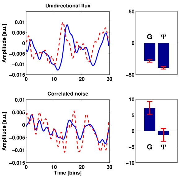
Figure 1: Upper panels: strong interaction from second (red in left panels) to first (blue in left panels) signal. Lower panels: mixture of brown and white noise. The error bars in the right panels indicate estimated 95% error margins corresponding to 2 standard deviations. Time series in the left panels were upsampled to 400 Hz.

To study a more general class of signals we simulated data with structure

$${\bf y}(t)=(1-\gamma)\frac{{\bf x}(t)}{N_{x}}+\gamma\frac{B{\bf\eta}(t)}{N_{\eta}}$$ (7)

Here, the signal ${\bf x}(t)$ contains truly unidirectional information flux and is generated using AR-models of order $P=5$ for two channels. In general, an AR-model is defined as

$${\bf z}(t)=\sum_{p=1}^{P}A(p){\bf z}(t-p)+{\bf\xi}(t)$$ (8)

where $A(p)$ are the AR-matrices up to order $P$ and $\xi(t)$ is white Gaussian noise with covariance matrix $\Sigma$ chosen here to be the identity matrix. For computing Granger Causality, the AR model was fitted with order $P=10$.

All entries of AR-matrices were selected randomly as independent Gaussian random numbers with $A_{21}(p)=0$ for the signal part ${\bf x}(t)$, corresponding to unidirectional flow from the second to first signal, and $A_{12}(p)=A_{21}(p)=0$ for the noise part ${\bf\eta}(t)$, corresponding to independent sources. Noise was mixed into channels with a random $2\times 2$ mixing matrix $B$. Both the signal part and the mixed noise part ($B{\bf\eta}(t)$) are normalized by the Frobenius norms of the respective data matrices ($N_{x}$ and $N_{\eta}$) and finally added with a parameter $\gamma$ controlling for the relative strength. The time constant implicit in the AR-model was assumed to be 10 ms, and we generated 60000 data points for each system and channel. This corresponds to a Nyquist frequency of 50 Hz and to 10 minutes measurement. We analyzed systems for all $\gamma$ in the range $[0,1]$ with step $0.1$. For each $\gamma$ we analyzed 1000 randomly selected stable systems with both methods and both for wide band (using all frequencies) and narrow band analysis. For the narrow band, we used a band of 5 Hz width, centered this band around the spectral peak of the (known) signal of interest and analyzed only cases where the band includes at least 60% of the total power of the signal of interest.

Figure 2: Fraction of significant detections of Granger Causality and PSI as a function of noise level $\gamma$.

The fractions of significant false and significant correct detections as a function of $\gamma$ are shown in Fig.2. We observe that for increasing noise level the fraction of significant false detections for Granger Causality comes close to $50\%$ while PSI rarely makes significant false detection at all. For PSI, the worst case observed is at $\gamma=0.8$ for the wide band with $6\%$ significant false detections. This level can be reduced to about $3.5\%$ if we increase the frequency resolution to $0.25$Hz. However, the price is some loss in statistical power and it is important to show that also the proposed method might fail, even if it is unlikely in the sense of the present simulation.

We observe similar significant correct detection rates for both methods for small and moderate noise levels. For high noise level Granger Causality shows a much larger fraction of significant correct detections which, however, is meaningless given the large fraction of significant false detections.

After having illustrated the robustness of our new method on simulated data we now apply the PSI to real data, namely EEG. For this, 88 healthy subjects were recruited randomly by the aid of the Swedish population register. During the experiment, which lasted for 15 minutes, the subjects were instructed to relax and keep their eyes closed. Every minute the subjects were asked to open their eyes for 5 seconds. EEG was measured with standard 10-20 system consisting of 19 channels. Data were analysed using linked mastoids reference. The protocol was approved by the Hospital Ethics Committee.

The most prominent feature of this measurement is the alpha peak at around 10 Hz. This rhythm is believed to represent a cortico-cortical or thalamo-cortical interaction. The direction of this interaction is an open question. While it is mostly believed that this rhythm originates in occipital areas and spreads to other (more frontal) areas da Silva (1991) this view has also been challenged Ito et al. (2005).

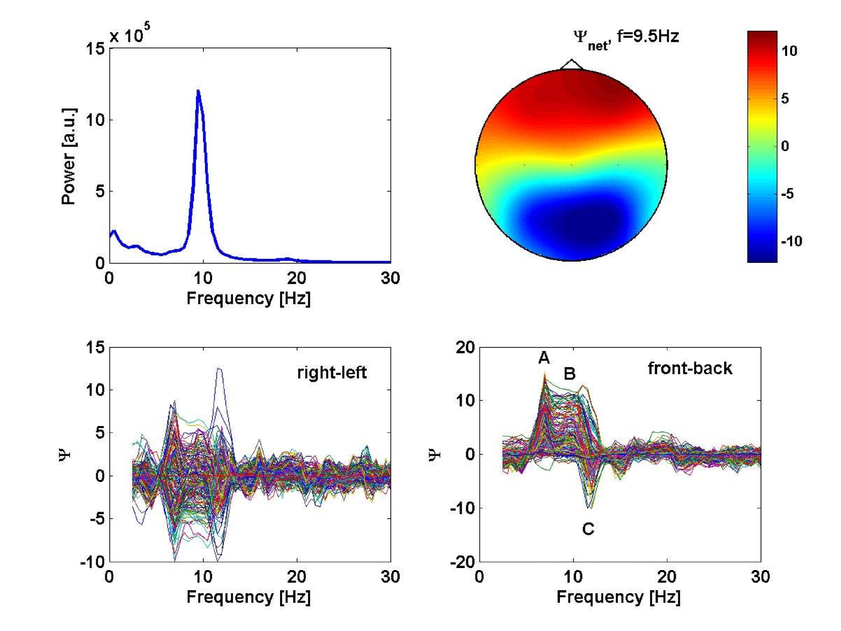
Figure 3: Upper left: signal power as a function of frequency averaged over the two occiptial channels O1 and O2 showing a clear alpha peak at $f=9.5$ Hz. Upper right: net information flux at $f=9.5$ Hz. Lower panels: PSI for all channel pairs and all frequencies projected on right-to-left and front-to-back direction, respectively.

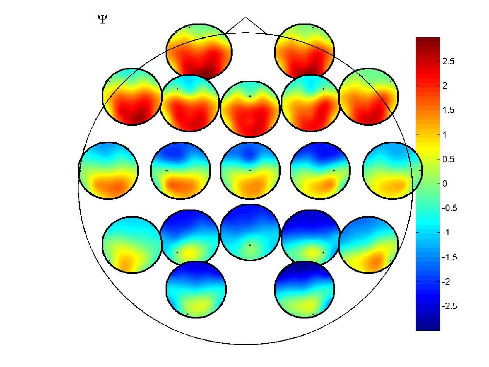
Figure 4: Phase Slope Index for all pairs of channels averaged over all subjects each at the peak of the alpha rhythm. The $i.th$ small circle is located at the $i.th$ electrode position and is a contour plot of the $i.th$ row of the matrix with elements $\Psi_{ij}$. The red color in frontal circles indicates that the frontal electrodes are estimated as the drivers.

For illustration we show results for PSI for one selected subject in Fig.3. The power (upper left panel), averaged over the two occipital channels (O1 and O2), shows a very strong peak at $9.5$ Hz. PSI values were calculated for all channel pairs with frequency resolution $0.5$ Hz using a frequency band of $5$Hz width centered around frequency $f$. In the upper right panel we show the net information flux at $f=9.5$ Hz defined for the $i.th$ channel by

$$\Psi_{net}(i,f)=\frac{\sum_{j}\Psi_{ij}(f)}{std(\sum_{j}\Psi_{ij}(f)}$$ (9)

We clearly observe that frontal channels are net drivers ( $\Psi_{net}>0$) and occipital channels net recipients ($\Psi_{net}<0$).

To show prefered direction for all pairs of channel and for all frequencies we calculate the respective contribution to a given direction in the following way: for channels $i$ and $j$ with locations ${\bf r}_{i}$ and ${\bf r}_{j}$ in the two dimensional plane (as shown in the upper right panel) respectively, we calculate the normalized difference vector

$$\delta{\bf r}_{ij}=\frac{{\bf r}_{j}-{\bf r}_{i}}{|{\bf r}_{i}-{\bf r}_{j}|}$$ (10)

and project it onto the direction of interest, i.e. onto ${\bf u}=(-1,0)^{T}$ for right to left direction and onto ${\bf u}=(0,-1)^{T}$ for front to back direction. We finally calculate the contribution of $\Psi_{ij}(f)$ to direction ${\bf u}$ as

$$\Psi_{i,j}(f,{\bf u})=\Psi_{ij}(f){\bf u}\cdot\delta{\bf r}_{ij}$$ (11)

Results for all channel pairs and for all frequencies are shown for right-left information flow (lower left panel) and for front-back information flow (lower right panel). We do not observe any prefered direction in the right-left flow. In contrast, the information flow in front-back direction shows a clear positive plateau at the alpha-frequency (indicated with letter ’B’) meaning that typically the frontal channels are estimated as the drivers. We also observe a positive and negative peak (indicated with letters ’A’ and ’C’) at frequencies around 7 Hz and 12 Hz, respectively. Note that these peaks differ by the width of the frequency band. They are clearly artefacts due to inadequate settings of the band. Specifically, the alpha rhythm has a prefered phase (for given channel pair) which is irrelevant for the estimation of the phase slope unless the alpha-peak is right at the edge of the frequency band such that the band covers only half of the system.

We found a similar structure in about 60% of the subjects. An average over all subjects now showing information flux between all subjects is shown in Fig.4. We also found a substantial inter-subject variability, both with regard to PSI and actual phase at the alpha peak. The origin is interesting but so far unclear and goes beyond the scope of this letter. Note that Granger Causality did not yield any consistent spatial pattern, presumably for reasons of high false negative rates similar to the ones observed in Fig.2.

Recent neuroimaging studies have challenged a simple view on a rest condition by showing a presence of default states in the cortex, which display complex patterns of neuronal activation Laufs et al. (2003); Mantini et al. (2007). We here show that not only specific areas are co-activated during rest state, but they also demonstrate at a gross level a preferential ”default” mode of information flow in the cortex. Importantly, the drivers of such flow are mostly situated in the frontal areas, from where many top-down attentional influences are thought to be originated Gilbert and Sigman (2007). In agreement with the above mentioned imaging studies, our study suggests that the maintenance of vigilance is a process displaying a coordination of neuronal activity with well defined drivers and recipients of information flow.

To conclude, we presented a new method to estimate the direction of causal relations from time series’ based on the phase slope of the cross-spectra. While it is well known that this slope is an indicator of the direction, the crucial point here is that we defined an average of the phase slope such that this average is insensitive to arbitrary mixtures of independent sources with arbitrary spectra.

We verified the claimed properties of the PSI for random linear systems also showing that the most prominent method to estimate direction of information flow, Granger Causality, is highly sensitive to mixtures of independent noise sources. Additionally, we showed that in situations with combined unidirectional flow and undirected noise our method correctly distinguished the two phenomena - in sharp contrast to Granger Causality. A final application of our method to real EEG data shows significant and meaningful results from the neurophysiological point of view and underlines the versatility of our new method as a universal tool for estimating causal flow in complex physical systems that consist of mixtures of subcomponents.

Acknowledgements. We acknowledge partial funding from DFG, BMBF and EU.

References

- Granger [1969] C. Granger, Econometrica 37, 424 (1969).
- Granger [1980] C. Granger, Journal of Econ. Dynamics Control 2, 329 (1980).
- Kaufmann and Stern [1997] R. Kaufmann and D. Stern, Nature 388, 39 (1997).
- Narayan and Smyth [2006] P. Narayan and R. Smyth, Applied Economics 38, 563 (2006).
- Marinazzo et al. [2006] D. Marinazzo, M. Pellicoro, and S. Stramaglia, Physical Review E 73, No.066216 (2006).
- Brovelli et al. [2004] A. Brovelli, M. Ding, A. Ledberg, Y. Chen, R. Nakamura, and S. Bressler, Proceedings of the National Academy of Sciences of the United States of America 101, 9849 (2004).
- Sato et al. [2006] J. Sato, E. Amaro, D. Takahashi, M. Felix, M. Brammer, and P. Morettin, Neuroimage 31, 187 (2006).
- Albo et al. [2004] Z. Albo, G. D. Prisco, Y. Chen, G. Rangarajan, W. Truccolo, J. Feng, R. Vertes, and M. Ding, Biol. Cybern. 90, 318 (2004).
- Nolte et al. [2004] G. Nolte, O. Bai, L. Wheaton, Z. Mari, S. Vorbach, and M. Hallett, Clin. Neurophysiol. 115, 2292 (2004).
- Nolte et al. [2006] G. Nolte, F. Meinecke, A. Ziehe, and K. Müller, Phys Rev E 73, 051913 (2006).
- Nunez et al. [1997] P. Nunez, R. Srinivasan, A. Westdorf, R. Wijesinghe, D. Tucker, R. Silberstein, and P. Cadusch, Electroencephalogr. Clin. Neurophysiol. 103, 499 (1997).
- Ding et al. [2006] M. Ding, Y. Chen, and S. Bressler, in Handbook of Time Series Analysis (Whiley, 2006), pp. 437–459.
- Marple [1987] S. Marple, Digital Spectral Analysis with Applications (Prentice Hall, Englewood Cliffs, NJ, 1987).
- [14] A. Schlögl, BIOSIG - an open source software library for biomedical signal processing, http://BIOSIG.SF.NET.
- da Silva [1991] F. L. da Silva, Electroencephal. and Clin. Neurophys. 79, 81 (1991).
- Ito et al. [2005] J. Ito, A. Nikolaev, and C. van Leeuwen, Biol. Cybern. 92, 54 (2005).
- Laufs et al. [2003] H. Laufs, K. Krakow, P. Sterzer, E. Eger, A. Beyerle, A. Salek-Haddadi, and A. Kleinschmidt, Proc Natl Acad Sci USA 100, 11053 (2003).
- Mantini et al. [2007] D. Mantini, M. Perucci, C. D. Gratta, G. Romani, and M. Corbetta, Proc Natl Acad Sci USA 104, 13170 (2007).
- Gilbert and Sigman [2007] C. Gilbert and M. Sigman, Neuron 54, 677 (2007).