Optimization and Scale-freeness for Complex Networks

Abstract

Complex networks are mapped to a model of boxes and balls where the balls are distinguishable. It is shown that the scale-free size distribution of boxes maximizes the information associated with the boxes provided configurations including boxes containing a finite fraction of the total amount of balls are excluded. It is conjectured that for a connected network with only links between different nodes, the nodes with a finite fraction of links are effectively suppressed. It is hence suggested that for such networks the scale-free node-size distribution maximizes the information encoded on the nodes. The noise associated with the size distributions is also obtained from a maximum entropy principle. Finally explicit predictions from our least bias approach are found to be born out by metabolic networks.

Networks galore! Representations of real complex systems in terms of networks range over all science from social science, economics, internet, physics, chemistry and biology and much more. Basically a network is a representation of who or what is connected to or influences whom or what. It takes the form of some irregular cobweb where the parts (the who’s or what’s) are connected by links. The parts are called nodes so the representation is in terms of nodes and links (see Fig.1). One feature of a network is the number of links which are attached to a node: a network can be characterized by $N(k)$, the number nodes with $k$ links attached to them. In many real networks one finds that this distribution over sizes $k$ is very broad and power law like i.e. $N(k)\sim k^{-\gamma}$. Why is this and what does it imply? This is still to large extent an open question. Here we adress this question using the maximum entropy principle. The predictive value of this principle is greatest when it fails! For example, when it was found that the measured blackbody radiation did have a smaller entropy than the one predicted from Maxwells equations and classical statistical mechanics, the maximum entropy principle (had it been known at the time) would immediately tell you that a physical constraint was lacking in the theory. This alas turned out to be the Planck constant. We use the same reasoning here: we first find that the maximum entropy for an unconstrained network does have a larger entropy than the broad distribution found in real systems. So there is a missing contraint! We argue that this missing contraint is the advantage (in many cases) of maximizing the information encoded on the nodes. Thus we are suggesting that the real advantage is not to maximize the total number of possibilities but rather to maximize the information encoded on the nodes. Our ”least bias” approach gives explicit predictions for real networks which can be tested. We demonstrate that metabolic networks (a network representation of the metabolism in a cell) are likely to be a maximum information network.

Complex networks have undergone a rapid surge of interest and a number of review articles already exist Albert and Barabási (2002)Dorogovtsev and Mendes (2003)Newman (2003)Boccaletti et al. (2006). A striking observation in this field is that many real networks have a broad scale-free like degree distribution. Why is this and what does it imply for the evolution mechanism of the networks? There exists many suggestions Albert and Barabási (2002)Dorogovtsev and Mendes (2003)Newman (2003)Boccaletti et al. (2006). Most suggestions concerns steadily growing networks. The most well-known proposal for an evolution mechanism which produces a scale-free network for this case is the preferential attachment scenario Barabási, Albert and Jeong (1999). This mechanism rests on two explicit assumptions: 1) a link on a new node attaches randomly to a node belonging to the network with a probability directly proportion to the number of links that are already attached to this latter node. 2) once a link is in place it stays in place. Although this model mechanism has become a successful prototype explanation in many cases Albert and Barabási (2002), its applicability is obviously limited by the very specific model assumptions. Other suggestions are based on various optimization ideas Valverde et al. (2002), and, finally, some concern non-growing networks Kim et al. (2005)Thurner and Tsallis (2005)Bianconi (2006).

In the present paper we discuss non-growing networks. Such a network has a fixed number of nodes and links and the time-evolution is through rewiring of links. First we discuss the definition of a random network. Next we address the question ”What is the least bias needed to impose on a random network in order to obtain a scale-free distribution?”. The possible ”least bias” solutions are presented together with the corresponding noise. Finally characteristic features arising from the ”least bias” random scale-free network are extracted and compared to real metabolic networks. Some speculations are added. Our approach is based on information theory and statistical mechanics Jaynes (1957).

I Randomness and States

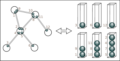
Figure 1: Figure showing how an undirected network can be described by numbered balls placed in boxes. The balls represent link-ends and are distinguishable because each link start and end on a specific node.

In statistical mechanics random means that each possible state of a system is equally probable. Consequently, one first has to identify what is meant by a state before the concept of randomness takes on a precise meaning. Here we will follow Ref. Jaynes (1957) by making the connection between states and different distinguishable ways of distributing objects. For example the lower right hand box in Fig.1 contains four distinguishable (numbered) balls. There are $4!=24$ ways in which these four balls can be distributed into the box. All these ways are distinguishable because the balls are distinguishable and thus correspond to $24$ different states. This is just like the box contained four different compartments each of which can contain one ball.

Figure 1 shows a non-directed network in terms of undirected links and nodes. Each link starts and ends with a link-end. Let us consider the link-ends on a node. In statistical mechanics one could think of the link-ends as particles. Since each link-end on a particular node is connected to another link-end on a different node, it means that the link-ends on a node are de facto distinguishable. Thus the closest analogy with statistical mechanics is that of boxes (nodes) containing distinguishable balls (link-ends). A first description of the system is then in terms of balls in boxes Bialas et al. (2000)Burdas et al. (2001). In addition there are constraints imposed by the network topology. Typical constraints are no loops (links starting and ending on the same node), at most a single link between two nodes, and keeping the network connected. A necessary (but not sufficient) constraint corresponding to connected networks is that each box always contains at least one ball. The other two constraints are often unimportant and occurs with a vanishing probability in the limit of large random networks Dorogovtsev and Mendes (2003). However, sometimes the no-loop constraint is crucial, as will be discussed further on.

II Balls in Boxes

Let us start with randomly distributing $M$ distinguishable balls into $N$ boxes. The total number of ways of picking the balls are $M!$ and the outcome is a distribution into the $N$ boxes where $N(k)$ boxes has $k$ balls. Since all the balls are distinguishable all boxes with $k$ balls are distinguishable and consequently the number of distinguishable ways of distributing the balls into the boxes, $\Omega,$ are given by

$$\ln\Omega = \ln M!-\sum_{k=0}\ln N(k)!$$ (1)

$$\eqsim M\ln M-M-\sum_{k=0}N(k)[\ln N(k)-1]$$ (2)

The degeneracy expressed by $N(k)!$ reflects the trivial fact that two boxes which contain the same number of balls have indistinguishable sizes. The connection to statistical physics is the one-to-one correspondence between distinguishable ways of distributing the balls and the states of the system Jaynes (1957). The unbiased estimate of the total number of different states $\Omega$ is given by the maximum of $\ln\Omega$ with respect to the distribution $N(k),$ subject to the constraints $\sum_{k=1}^{N}N(k)=N$ and $\sum_{k=1}^{N}kN(k)=M$. This gives by variational calculus $-\ln N(k)+a-bk=0$ with the solution

$$N(k)=A\exp(-bk)$$ (3)

[$a$ and $b$ are the Lagrange multipliers corresponding to the constraints and $A$ is a normalization constant corresponding to $\sum_{k}N(k)=N$]. This is the exponential distribution which within statistical physics in other variables can be recognized as the well-known Boltzmann distribution.

Suppose now that the balls instead are indistinguishable. In this case the boxes can only be distinguished if the number of balls they contain are different. Compared to the case with distinguishable particles this means that all ways of distributing $k$ balls into a box are indistinguishable or degenerate. We define the degeneracy $f(k)$ as the number of of ways of distributing balls into a box which are indistinguishable. This means that $f(k)$ is the total number of of ways of distributing $k$ different particles into a box divided by the total number of distinguishable states which the box can have. In the present example this is obviously $f(k)=k!/1$. Consequently total number of distingushable state are now

$$\ln\Omega= \ln M!-\sum_{k=0}\ln N(k)!-\sum_{k=0}N(k)\ln f(k)]$$

$$\eqsim M\ln M-M-\sum_{k=0}N(k)[\ln N(k)-1+\ln k!]$$ (4)

and the unbiased estimate is again given by maximizing $\Omega$ with respect to the distribution $N(k)$. The variational solution in this case gives $-\ln N(k)-\ln k!+a-bk=0$, and thus $N(k)\sim\exp(-bk)/k!\sim const^{k}/k!$. This is the Poisson distribution which in the context of networks is associated with the random Erdős-Renyi (ER) network.

As mentioned above a connected network corresponds to the case when all boxes contain at least one ball. How does this constraint change the distribution? It corresponds to first filling all the boxes with precisely one ball. The number of ways of doing this is $M!/(M-N)!$. The number of ways to fill in the remainder is given by

$$\ln(M-N)!-\sum_{k=1}\ln N(k)!-\sum_{k=1}N(k)\ln f(k).$$ (5)

Thus the crucial question is how the degeneracy $f(k)$ changes. Let us start with ER-case and indistinguishable balls. The degeneracy $f(k)$ is this time given by the number of distinct ways to fill a box with distinguishable balls divided by the number of distinguishable ways to fill a box will the remaining $k-1$ balls. For indistinguishable balls this is simple. There is only one distinguishable way to fill a box with $k-1$ indistinguishable balls. Consequently, $f(k)=\frac{k!}{1}$ and the distribution has again the Poisson-distribution form.

The case of distinguishable balls is in this respect quite different: the number of distinguishable ways to fill a box with $k-1$ distinguishable balls is obviously $(k-1)!$ and consequently the degeneracy is now $f(k)=\frac{k!}{(k-1)!}$. Thus the total number of distinguishable ways of distributing distinguishable balls subject to the constraint that all boxes contains at least one ball is given by

$$\ln\Omega= \ln M!-\sum_{k}\ln N(k)!-\sum_{k}N(k)\ln k$$

$$\eqsim M\ln M-M-\sum_{k}N(k)[\ln N(k)-1+\ln k].$$ (6)

The unbiased estimate of the total number of different states $\Omega$ is given by the maximum of $\ln\Omega$ with respect to the distribution $N(k),$ subject to the constraints $\sum_{k=1}^{N}N(k)=N$ and $\sum_{k=1}^{N}kN(k)=M$ which by variational calculus gives $-\ln N(k)-\ln k+a-bk=0$ with the solution

$$N(k)=\frac{A\exp(-bk)}{k}$$ (7)

By this reasoning an unbiased random connected network has a degree-distribution of the form

$$P(k)=\frac{N(k)}{N}\sim\frac{\exp(-bk)}{k}$$ (8)

To sum up: We use the correspondence between the different ways to distribute balls and states in statistical mechanics. Taking this into account gives more possible states for distinguishable than for indistinguishable balls. The link-ends on a node correspond to distinguishable balls. An unbiased estimate assumes that all these states are equally probable. This leads to a degree-distribution $P(k)\sim\exp(-bk)/k$ which is distinctly different from the Poisson distribution.

How close is the analogy between distinguishable-balls-in-boxes (DBB) model and a network? If we define a link by its link-ends such that an enumeration of them are given by $(1,2),(3,4),...,(M-1,M)$ then the mapping is precise. However, not all possible distributions of links fulfill the requirement for a network. As pointed out above, the difference imposed by the network constraints on the states of the DBB-model are often of minor importance, except for the no-loop constraint which can be crucial. An example when the no-loop condition makes a crucial difference between the DBB-model and the corresponding network is the star-like networks (or more generally networks which contain nodes of order $M$): the number of possible states for such networks are significantly smaller in comparison with the number of the corresponding DBB-states.

We note that a necessary but not sufficient (because the orderings of the objects in a box corresponds to different states) condition for two states to be equal is that they contain precisely the same boxes provided a box is identified by the specific balls it contains; for two equal DBB-states all the boxes corresponding to the one state can be put on top of identical boxes corresponding to the other. Likewise for two equal states of a network: the two networks corresponding to the equal states can be put on top of each other so that all nodes and all links precisely match.

How should one actually fill the boxes with balls in case of the constrained DBB-model? One starts with one ball in each box. Next one randomly chooses one of the remaining $M-N$ balls and add another ball in an arbitrary box. This box is chosen with the probability $p(k=1)\sim 1$, $p(k>1)\sim k-1$ in order to ensure that all the possible states are given the same chance. It follows that

$$p(1) =\frac{1}{N(1)+\sum(k-1)N(k)}$$

$$p(k>1) =\frac{k-1}{N(1)+\sum(k-1)N(k)}$$

Throwing the balls into the boxes according to the above probability distribution gives the unbiased distribution $P(k)\sim\exp(-bk)/k$ (for $k>1$). If the balls are already in the boxes and one wants to choose all possible states with equal probability, then one have to use the procedure of choosing two balls randomly and then move the one to the same box as the other Minnhagen et al. (2005). We also note in passing that for the unconstrained DBB-model, the probability reduces to $p(k)\sim k$ which has the form of a preferential attachment to boxes. However, in our context it arises as a direct statistical consequence of distinguishable balls and in fact represents the unbiased situation with no preference what so ever!

III Box Information and Scale-freeness

So far we have argued that the random distribution for a network is given by $P(k)\sim\exp(-bk)/k$. What type of bias in the sampling of different states are necessary for changing the degree-distribution to a power law $P(k)\sim k^{\gamma}$ and what is the least bias necessary? To this end we consider the box information (the information contained within a box) of the DBB-model. The box (or ”useful”) information, $s_{in}$, contained in a box with distinguishable particles is given by the logarithm of the number of possible different orderings of the balls within the boxes. For the unconstrained DBB model this is $s_{in}=\ln k!$, while for the constrained DBB-model it is $s_{in}=\ln(k-1)!$. The total box information for the unconstrained DBB-model is hence $S_{in}=\sum_{k}N(k)\ln k!$. Note that this is the maximum box information you can store for a given distribution $N(k)$. The global maximum is trivially the case when all balls are in the same box i.e. $N(M)=1$ and $N(k<M)=0$ so that $S_{in}^{\max}=\ln M!$. For the constrained DBB-model we instead have $S_{in}=\sum_{k}N(k)\ln(k-1)!$ with the global maximum $S_{in}^{\max}=\ln(M-N+1)!$ for $N(M-N+1)=1$ and $N(1)=N-1$. The difference between the total box information for the unconstrained DBB-model, i.e. the maximum box information you can store for a given distribution $N(k)$, and the total box information for the constrained DBB-model (divided by the number of boxes to get an intensive quantity) is

$$\Delta S_{in}=\frac{1}{N}\sum_{k=1}N(k)\ln k.$$ (9)

Thus small $\Delta S_{in}$ means large box information. It seems plausible to us that a bias towards large box information could be favored in various contexts and will hence consider how such a bias will affect the network degree-distribution.

In order to find the distribution $N(k)$ which corresponds to the smallest $\Delta S_{in}$ we do a variational calculation: In addition to the basic constraints for a non-growing network, $\sum_{k=1}^{N}P(k)=1$ and $\sum_{k=1}^{N}kN(k)=M/N$, we then also have the constraint $\Delta S_{in}[P(k)]=B$. The fixed information value, $B$, introduces a bias on the purely random states. This biased $P_{B}(k)$ is obtained by maximizing the number of different states, subject to the three constraints. These constraints are handled by three Lagrange multipliers and the solution is the one which maximizes

$$-\sum_{k}P_{B}(k)[\ln P_{B}(k)+a+bk+c\ln k]$$ (10)

with respect to the distribution $P_{B}(k)$. This leads to

$$P_{B}(k)=\frac{A\exp(-bk)}{k^{c}}$$ (11)

where the constant $A$, $b$, and $c$ are given by the three constraints. From the normalization condition $\sum_{k=1}^{N}P_{B}(k)=1$ we directly get $A(b,c)$ and the remaining constants $b$ and $c$ are obtained from the remaining two constraints. Figure 2(a) shows how $b$ and $c$ depend on the ratio $M/N$. The possible solutions ranges from $(1\leq c<c_{0},\ b>0)$ to $(c=c_{0},\ b=0)$ i.e. from $P(k)\sim\exp(-bk)/k^{c}$ to $P(k)\sim k^{-c_{0}}$, where $c_{0}=c_{0}(N,M/N)$. [Note that $c_{0}>2$ for large N because of the normalization condition]. Using the explicit form of the solutions it is easy to show that for $M$ balls and $N$ boxes the scale-free distribution corresponds to the smallest $B$ and hence to the largest box information for the ”least bias” solutions (see Fig. 2(b))Least bias (2006).

The relation between the global maximum solutions mentioned above (which are not obtained within variational calculus) and networks will be discussed in the following. Our conclusion will be that the scale-free network corresponds to the global maximum of node information.

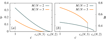
Figure 2: Figure showing how the Lagrange multiplier $b$ (Fig. a) and the box information difference $B$ (Fig. b) depend on $c$ for two different average number of balls ($2$ and $3$) and $N=10^{6}$. Here, $c_{0}(N,2)=2.41$ and $c_{0}(N,3)=2.15$.

IV Scale-freeness and Noise

The degree distributions $P(k)$ are average distributions. This means that, if $p_{i}$ is the probability for a possible distinct system state $i$, then the average distribution $P(k)$ is given by $P(k)=\sum_{i}p_{i}N_{i}(k)/N$ $=\langle n(k)\rangle$, where the sum is over all box distributions corresponding to the system states $i$ (denoted by $\langle\rangle$). We have so far only characterized the system by the average box distribution $\langle n(k)\rangle$. Our goal is to find as detailed characteristics as possible for the maximum node-information random scale-free network, in order to be able to decide whether or not a particular network obeys the statistical properties implied by this particular random scale-free network. To this end we also derive the statistical deviations from the average distribution $\langle n(k)\rangle$. This statistical deviation is measured by the noise

$$\sum_{k}\langle(n(k)-\langle n(k)\rangle^{2}\rangle.$$ (12)

The actual calculation follows the same steps as the variational calculation of the maximum box information scale-free network in the previous section. Again we address the problem of imposing the fixed information constraint $\Delta S_{in}=B$ into the DBB-model

$$B=\sum_{k}P(k)\ln k=\langle\sum n(k)\ln k\rangle=\sum_{i}p_{i}\sum_{k}n_{i}(k)\ln k$$ (13)

Thus our constraints are now a fixed value $B,$ $\sum_{i}p_{i}=1$ and $\sum_{i}p_{i}\sum_{k}n_{i}(k)k=M/N.$ We want to maximize the average number of distinct states $\Omega$ or equivalently

$$\ln\Omega=const-\sum_{i}p_{i}\sum_{k}n_{i}(k)\ln[n_{i}(k)k]$$ (14)

(see Eq. (6)). With no bias the problem just corresponds to maximizing the entropy $-\sum_{i}p_{i}\ln p_{i}$ subject to the constraint $\sum_{i}p_{i}=1$ Jaynes (1957): the unbiased value of the probability for a state is the maximum of $-\sum_{i}p_{i}[\ln p_{i}+const]$ with respect to variations of $p_{i}$. The answer is obviously that all $p_{i}$ are equal i.e. all system states are equally probable. Note that the variation is now with respect to the probabilities $p_{i}$ of the system states $i$, whereas in the previous sections it was with respect to the average distributions $P(k)$. For fixed values of $B$, $\Omega$ and $M/N$ the problem instead corresponds to finding the maximum of the expression (where $\alpha$, $\beta$, $\gamma$ and $\delta$ are Lagrange multipliers).

$$-\sum_{i}p_{i}[\ln p_{i}-\alpha\sum_{k}n_{i}(k)\ln k+\beta\sum_{k}n_{i}(k)\ln[n_{i}(k)k]$$

$$+\gamma\sum_{k}n_{i}(k)+\delta\sum_{k}n_{i}(k)k],$$ (15)

with respect to variations of $p_{i}$. We here use different symbols for the multipliers than in previous sections in order to emphazise that the variations are with respect to a different variable. The result is straightforwardly obtained and gives the probabilty for a system state $i$ as an exponential $p_{i}\sim\exp(-H/T)$ where

$$\frac{H}{T}= -\alpha\sum_{k}n_{i}(k)\ln(k)+\beta\sum_{k}n_{i}(k)\ln[n_{i}(k)k]$$

$$+\gamma\sum_{k}n_{i}(k)+\delta\sum_{k}n_{i}(k)k$$ (16)

Here we used the notation $\frac{H}{T}$ for the function in the exponent in order to display the equivalence with statistical physics and the Boltzman factor: in statistical physics the probability of a system state $i$ is given by $p_{i}=Z^{-1}\exp(-H/T)$ where $H$ is the hamiltonian, $T$ is the temperature and $Z^{-1}$ is a the normalization constant determined by the condition $\sum_{i}p_{i}=1$. In statistical physics $Z$ is called the partition function. The average value of any quantity $O(n(k),k)$ is given by $\langle Z^{-1}\exp(-H/T)O(n(k),k)\rangle$ where the brackets means the average over all different states. For the DBB-model the two last constraints in Eq.(16) (i.e. constant number of boxes and balls) are included already in the definition of the model, so the Hamiltonian $H$ reduces to

$$\frac{H}{T}=\frac{1}{T}[\sum_{k}n(k)\ln n(k)+\gamma_{0}\sum_{k}n(k)\ln k]$$ (17)

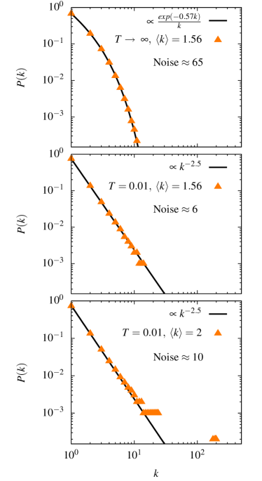
Figure 3: Distribution of box-sizes obtained by Monte Carlo simulations where the Hamiltonian from Eq. 17 was used. $N=1000$, $\gamma_{0}=2.5$ and the results were averaged over $2000$ runs. Figure (a) and (b) shows the results for an average number of balls equal to $1.56$ and $T$ reaching infinity and zero respectively. In (c), $T$ is also close to zero but $M/N=2$ and boxes (nodes) of order $M$ is forming. Note that the Scale-free distribution (b) has the smallest noise.

with $T=1/\beta$ and $\gamma_{0}=(\beta-\alpha)/\beta$. This system state probability and Hamiltonian in the network context was first derived and investigated in Ref. Minnhagen et al. (2005). In particular Monte-Carlo simulations are easily implemented following the standard proceedure in statistical physics: choose two random balls and then move one to the same box as the other with a probability given by the Boltzmann factor $\exp(-H/T)$. Figure 3(a) shows the unbiased estimate obtained from MC simulations which obviously corresponds to $T=\infty$ and also $\alpha=0$ (= no bias). This is just the unconstrained DBB-model and the average distribution is of the form $P(k)\sim\exp(-\delta k)/k$ as previously shown. The new characteristics is the statistical deviations from the average distribution, the noise, associated with the least bias (which in this case is no bias at all). The least bias always corresponds to the smallest ratio $\alpha/\beta$ in Eq. (16) and hence to the largest $\gamma_{0}$ in Eq. (17) for which the average solution of the form $P(k)\sim\exp(-\delta k)/k^{\gamma}$ with $1\leq\gamma<\gamma_{0}$ is obtained. It turns out that for each given ratio $M/N$ there is precisely one such largest value $\gamma_{0}$ which is given by the condition

$$C\equiv\frac{\sum_{k=1}^{N}kk^{-\gamma_{0}}}{\sum_{k=1}^{N}k^{-\gamma_{0}}}=M/N$$ (18)

(note that $\gamma_{0}=c_{0}(N,M)$ where $c_{0}(N,M)$ is defined in the preceding section). This also means that the statistical noise for the whole sequence of least biased solutions is uniquely given. Since $\gamma_{0}$ is unique the noise is just given by the ”temperature” $T$ : large noise corresponds to large $T$ and small noise to small, which is, of course, precisely what you would expect from statistical physics. The scale-free distribution is obtained in the limit of small $T$ and consequently has the smallest noise. Figure 3(b) shows the average distribution and the noise obtained for a low $T$. The important point is the connection between the scale-free distribution and the smallest noise.

What do the two cases $C>M/N$ and $C<M/N$ correspond to? In the first case the average distribution is of the form $P(k)\sim\exp(-\delta k)/k^{\gamma}$ with $\delta>0$. So the solutions overlap with the ones obtained for the least bias. The point is that these solutions are obtained for a smaller $\gamma_{0}$ and hence for a larger bias. This means the same $P(k)$ but a smaller noise. The case $C<M/N$ means that $\gamma_{0}$ is larger than for the least bias solutions. In this case boxes with of order $M$ balls are created. An example is given in Fig. 3(c). Note that these solutions with order $M$ nodes are not picked up by variational calculus.

For the network, the presence of nodes of order $M$ greatly constrains the number of possible different states relative to the DBB-model, because of the no-loop constraint. For example a perfect star with $N$ nodes and $M=2(N-1)$ link-ends [ $N-1$ single nodes attached to a central node of degree $N-1)$] for the constrained DBB model corresponds to the box information

$$\Delta S_{in}=\sum_{k=1}P(k)\ln k\approx\frac{1}{N}\ln(N-1)\rightarrow 0$$ (19)

for large $N$. However, only one of these states is consistent with the network requirement so that

$$\Delta S_{in}\sim\frac{1}{N}[M\ln M-N\ln N]\approx\ln(N).$$ (20)

For a network this implies the solutions containing order $M$ nodes will always have much smaller node information than the corresponding scale-free network.

Based on these observations, we conjecture that the scale-free network maximizes the node information.

V Consequences for Directed Networks.

So far we discussed undirected networks. However, also directed networks has a one-to-one mapping to the constrained DBB-model. In this case a link is again defined by two balls: if the balls are enumerated $1,2,,,M$ then the links are enumerated by two consecutive numbers $12,34,,,\ M-1M$ where the first number (which is always odd) denotes the start of the link and the last (even numbers) denote the end of the link. This does not change anything as to the number of different ways you can distribute the balls (or links) among the boxes (nodes). Thus the scale-free network should again be the one which maximizes the node information. Note that the direction of the links does not affect the amount of node information which a node can carry. Consequently, from the point of view of node information the directions of the links attached to a node are completely random. Thus a network, which is only optimized with respect to the node information, acquires characteristic random features with respect to the distribution of in-going and out-going links attached to a node.

Some of these characteristic random features for in- and out-links attached to a node are as follows: Suppose that the numbers of the in-, out-, and total numbers of links connected to a node are $k_{in},$ $k_{out}$, and $k$ , respectively, so that $k_{in}+k_{out}=k$. The average number of in-links $\langle k_{in}\rangle_{out}$ for for nodes with precisely the number of $k_{out}$ out-links are then given by the binomial coefficient $B(k_{in},k)$ i.e. the probability to get $k_{in}$ tails when tossing a coin $k=k_{\mathrm{in}}+k_{\mathrm{out}}$ times:

$$\langle k_{in}\rangle_{k_{\mathrm{out}}}=\frac{\sum_{k=k_{out}}^{k_{max}-k_{out}}B(k-k_{out},k)P(k)(k-k_{out})}{\sum_{k=k_{out}}^{k_{max}-k_{out}}B(k-k_{out},k)P(k)}.$$ (21)

For a the case of $P(k)\propto 1/k^{\gamma}$ one then finds $\langle k_{\mathrm{in}}\rangle_{out}\approx k_{\mathrm{out}}$ Bernhardsson and Minnhagen (2006). The result $\langle k_{\mathrm{in}}\rangle_{out}$ $\approx$ $k_{\mathrm{out}}$ may look innocent, but it is completely non-trivial, as realized when comparing to the ER-network: in this latter case there is no correlation and $\langle k_{\mathrm{in}}\rangle_{out}=const$ no matter what size $k_{out}$ one chooses. Another characteristic feature is the spread of the distribution of $k_{in}$-links for the nodes with a given number of $k_{out}$. For this spread we use the measure

$$S_{in}(k_{out})=\frac{\sum_{(k_{in}|k_{out})}|k_{in}-\langle k_{in}\rangle_{k_{out}}|}{\langle k_{in}\rangle_{k_{out}}}$$ (22)

which in terms of the binomial coefficient becomes

$$S_{in}(k_{out})=$$

$$\frac{\sum_{k=k_{out}}^{k_{max}-k_{out}}B(k-k_{out},k)P(k)\frac{k-k_{out}-\langle k_{in}\rangle_{k_{out}}}{\langle k_{in}\rangle_{k_{out}}}}{\sum_{k=k_{out}}^{k_{max}-k_{out}}B(k-k_{\mathrm{out}},k)P(k)}$$ (23)

This gives $S_{\mathrm{in}}(k_{\mathrm{out}})\propto k_{\mathrm{out}}^{-1/2}$,whereas for the ER-network the spread is independent of $k_{\mathrm{out}}$ i.e. $S_{\mathrm{in}}(k_{\mathrm{out}})=const$ Bernhardsson and Minnhagen (2006). From symmetry one has $P_{in}(k)=P_{out}(k).$ Using the relation $\langle k_{\mathrm{in}}\rangle_{out}$ $\approx$ $k_{\mathrm{out}}$ one can motivate the (at least) approximate relation

$$P_{tot}(k)\sim P_{in}(\frac{k}{2})=P_{out}(\frac{k}{2})$$ (24)

for even $k$, where $P_{tot}$, $P_{in}$ and $P_{out}$, are the size distributions of the tot-, in-, and out-links, respectively. This means that all three distributions are described by the same functional form $P(k)=P_{tot}(k)\sim P_{in}(\frac{k}{2})=P_{out}(\frac{k}{2}).$ The motivation steps are as follows:

$$P_{in}(k_{in}) =\sum_{k_{out}}P_{tot}(k_{out}+k_{in})\sim P_{tot}(\langle k_{out}\rangle|_{k_{in}}+k_{in})$$

$$\simeq P_{tot}(2k_{in})$$ (25)

Taking into account that $\sum_{k}P_{tot}(2k)$ only has half as many points as $\sum_{k}P_{in}(k)$ fixes the normalization constant to $2$ and thus leads to the relation

$$2P_{tot}(2k)=P_{in}(k)$$ (26)

The general connection between the total- and in-, out-link distributions,

$$P_{tot}(k_{tot})={\textstyle\sum\limits_{k_{in+k_{out}}=k_{tot}}}P_{in}(k_{in})P(k_{out}),$$ (27)

is then of the form

$$2\ P(2k)={\textstyle\sum\limits_{q=0}^{k}}P(q)P(k-q)\text{ \ \ \ }for\text{ \ }k\geqq 2.$$ (28)

Metabolic networks:

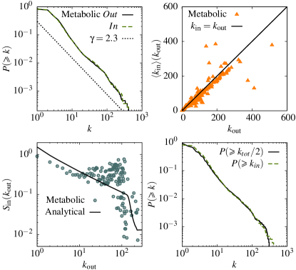
Figure 4: Metabolic Networks: Average over 107 metabolic networks with data obtained from Ref. (Ma et al. (2003)). The same characteristics as for Model A and Friendly Merging: a) Cumulative degree-distribution $P(\geq k)$. The dashed straight line line has the slope $\gamma=2.3$ and $\langle k_{in}\rangle=\langle k_{out}\rangle\approx 4.3$. b) Plot of $\langle k_{in}\rangle_{out}$ versus $k_{out}$ showing that the data is consistent with $\langle k_{in}\rangle_{out}=k_{out}$. c) Demonstration that the spread goes as $S_{in}(k_{out})\propto k_{out}^{-1/2}$ to reasonable approximation, full line from Eq. (23) and data points from simulations. The cut-off for large $k_{out}$ is a finite size effect. d) demonstrates that the relation $2P_{tot}(2k)=P_{in}(k)=P_{out}(k)$ is fulfilled as expected for a maximum-node-information network (note that $P(>k)=\sum_{k}^{k_{\max}}P(k)$).

These three characteristics can now be used to compare with real networks. As an illustration we choose metabolic networks:Bernhardsson and Minnhagen (2006) The data shown in Fig. 4 are average properties of 107 metabolic networks with the average size $\langle N\rangle\approx 940$ (data taken from Ref. Ma et al. (2003)Ma et al. (2003)). A metabolic network is constructed as follows: Substrates and products in the metabolism are nodes. Two nodes are connected if the substance of one is a substrate in a metabolic reaction which produces the substance represented by the other node. The links points from the substrate to the product. The data are obtained as the average over 107 such networks and consequently reflect an ensemble average network structure associated with metabolic networks. Figure 4(a) shows that metabolic networks have $P_{out}(k_{out})=P_{in}(k_{in})$ and also have a broad scale-free degree-distribution as was first demonstrated in Ref. Jeong et al. (2000). In addition from Fig. 4(b) and (c) we conclude for the ensemble average of metabolic networks the relation $\langle k_{in}\rangle\approx k_{out}$ holds to good approximation in accordance with the maximum node-information requirement. Likewise the spread has a similar decrease as required by maximum node information. Furthermore, Fig. 4(d) shows that the relation $2P_{tot}(2k)=P_{in}(k)=P_{out}(k)$ holds to excellent approximation [in accordance with standard practice in network analysis contexts, it is in Fig. 4(d) expressed in terms of the cumulant distribution $P(>k)=\sum_{k}^{k_{\max}}P(k)$]. Thus ensemble averages over metabolic networks show every sign of belonging to a maximum node-information network.

VI Concluding Remarks

In this paper we introduced and studied the constrained DDB-model. This model has a one-to-one mapping to a network provided the network is allowed to have loop-links and to be disconnected. We showed that the maximum box information state for the constrained DBB-model is a scale-free size-distribution of the boxes described by a power-law with an exponent $-\gamma$ with $\gamma>2$, provided the possibility of having boxes with a finite fraction of the balls are excluded (exclusion of order $M$ boxes). Next we observed that the presence of order $M$ nodes is effectively suppressed for connected networks with no loop-links. This led to the conjecture that the scale-free network gives the maximum node information. This conjecture in turn leads to explicit characteristic features for the scale-free maximum node-information network. We showed that an ensemble of metabolic networks has these features and concluded that metabolic network appears to have evolved in a way which maximizes the node information. The obvious question is then ”Why?”. We have at present no answer to this apart from the general observation that keeping as many options as possible increases the chances to adapt to new conditions. Neither has it escaped our notice that in the case of metabolic networks the ordering of the link ends on a node corresponds to a time-ordering and that further a particular time-ordering is required for creating a specific functional metabolic pathway. If this is the case one might speculate that maximum node information corresponds to the maximum number of potential metabolic pathways.

Acknowledgment 1

This work was supported by the Swedish research Council through contract 50412501.

References

- (1)
- (2)
- (3)
- (4)
- Albert and Barabási (2002) R. Albert and A.-L. Barabási, Rev. of Mod. Phys. 74, 47 (2002)
- Dorogovtsev and Mendes (2003) S. Dorogovtsev and J. Mendes, Evolution of Networks:From Biological Nets to the Internet and WWW (Oxford University Press, 2003)
- Newman (2003) M.E.J Newman, SIAM Review 45, 167 (2003).
- Boccaletti et al. (2006) S. Boccaletti, V. Latora, Y. Morena, M. Chavez, and D.-U. Hwang, Phys. Rep. 424, 175 (2006).
- Barabási, Albert and Jeong (1999) A.-L. Barabási, R. Albert, and H. Jeong, Science 286, 509 (1999).
- Valverde et al. (2002) S. Valverde, R.F. Cancho and R.V. Solé, Europhys. Lett 60, 512 (2002).
- Kim et al. (2005) B.J. Kim, A. Trusina, P. Minnhagen, and K. Sneppen, Eur. Phys. J. B 43, 369 (2005).
- Thurner and Tsallis (2005) S. Thurner and C. Tsallis, Europhys. Lett 72, 197 (2005).
- Bianconi (2006) G. Bianconi, cond-mat/0606365v5 (2006)
- Jaynes (1957) E.T. Jaynes, Phys. Rev 106, 620 (1957)
- Bialas et al. (2000) P. Bialas, L. Bogacz, Z. Burda, and A. Krzywicki, Nucl. Phys. B 575, 599 (2000).
- Burdas et al. (2001) Z. Burdas, J. Correia, and A. Krzywicki, Phys. Rev. E 64, 046118 (2001).
- Minnhagen et al. (2005) P. Minnhagen, S. Bernhardsson, and B.J. Kim, Submitted to Eur. Phys. Lett. (2006).
- Bernhardsson and Minnhagen (2006) S. Bernhardsson and P. Minnhagen Phys. Rev. E 74, 026104 (2006).
- Ma et al. (2003) H. Ma, and A.-P. Zeng, Bioinformatics 19, 270 (2003).
- Ma et al. (2003) H. Ma, and A.-P. Zeng, Bioinformatics 19, 1423 (2003).
- Jeong et al. (2000) H. Jeong, B. Tombor, R. Albert, Z.N. Oltvai, and A.-L Barabási, Nature 407, 651 (2000).
- Least bias (2006) The “least bias” solution corresponds to the largest number of states for a given value of the entropy see Ref. [13].