Nonlinear theory and tests of earthquake recurrence times

Abstract

We develop an efficient numerical scheme to solve accurately the set of nonlinear integral equations derived previously in (Saichev and Sornette, 2007), which describes the distribution of inter-event times in the framework of a general model of earthquake clustering with long memory. Detailed comparisons between the linear and nonlinear versions of the theory and direct synthetic catalogs show that the nonlinear theory provides an excellent fit to the synthetic catalogs, while there are significant biases resulting from the use of the linear approximation. We then address the suggestions proposed by some authors to use the empirical distribution of inter-event times to obtain a better determination of the so-called clustering parameter. Our theory and tests against synthetic and empirical catalogs find a rather dramatic lack of power for the distribution of inter-event times to distinguish between quite different sets of parameters, casting doubt on the usefulness of this statistics for the specific purpose of identifying the clustering parameter.

I Introduction

Most complex systems of interest in the natural and social sciences exhibit intermittent bursts of activity interspersed within long times of reduced activity. A simple metric to characterize this property consists in the distribution of recurrence (also called “waiting” or “inter-event”) times between (suitably defined) events. Recently, the literature has undergone itself a burst of publication activity on this topic, motivated by the idea that distributions of recurrence times may be one of the most important complexity measures for both random fields and nonlinear dynamical systems Gao . The applications include recurrence time and anomalous transport Zaslavsky91 , waiting times between earthquakes Corral03 ; Corral2004a ; Livina ; SaichevSor06 ; SaichevSor07 and rock fractures Davisenetal07 , time intervals between consecutive e-mails Barabasi_Nature05 and between web browsing, library visits and stock trading Vasquez_et_al_06 .

Much of the recent interest of the statistical physics community focused on applying scaling techniques, which are common tools in the study of critical phenomena, to the statistics of inter-earthquake recurrence times or waiting times Baketal02 ; Corral03 ; Corral2004a ; Corral2004b ; Corral2005a ; Corral2005b ; Corral2006 ; Corral_Christensen06 ; DavidsenGoltz04 ; Livina06 . Many of the claims made in these recent articles on recurrence statistics have either been challenged, refuted or explained by previously known facts about earthquake statistics Lindmanetal05 ; Lindmanetal06 ; Molchan05 ; Hainzl2006 ; SaichevSor06 ; SaichevSor07 . In particular, two of us SaichevSor06 ; SaichevSor07 have developed a general theory of the statistics of inter-event times in the framework of the general class of self-excited Hawkes conditional Poisson processes Hawkes71a ; Hawkes71b ; HawkesOakes74 adapted to modeling seismicity. The corresponding model is known as the epidemic-type aftershock sequence (ETAS) model, in which any earthquake may trigger other earthquakes, which in turn may trigger more, and so on. Introduced in slightly different forms by Kagan and Knopoff KK81 and Ogata Ogata88 , the model describes statistically the spatio-temporal clustering of seismicity. Using three well-known statistical laws of statistical seismicity (the Gutenberg-Richter, the Omori law and the productivity law), the empirical observations on the distribution of earthquake recurrence times can be explained within this model without invoking additional mechanisms other than the well-known fact that earthquakes can trigger other earthquakes SaichevSor06 ; SaichevSor07 .

A recent development is the proposition that inter-event time distributions may provide a new and more reliable way to measure of the so-called background earthquake activity Hainzl2006 ; Hardebeck07 . This question arises as follows: if earthquakes trigger other earthquakes, how much of the observed seismicity is due to past seismicity (endogenous origin) and how much is resulting from an “external” driving source (exogenous origin) often referred to as “background” seismicity thought to reflect the driving tectonic forces at large scales. This question obviously generalizes to any system in which future events may be in part triggered by past events, such as in commercial sales Sornetteetal04 and web browsing activity Vasquez_et_al_06 ; CraneSornette07 . Within the ETAS framework, the fraction of events in a given catalog which have been triggered by previous events can be shown Helmsor03 to be nothing but the so-called branching ratio $n$, defined mathematically as the average number of first-generation events triggered by a given preceding event Helmsor02 . Reciprocally, the fraction of background events is equal to $1-n$ (note that these models assume that the triggering branching-like processes are sub-critical: $n<1$). The degree to which the parameter $n$ can be retrieved from the distribution of inter-event times relies on departure from universality pointed out by Hainzl et al.Hainzl2006 and two of us SaichevSor06 ; SaichevSor07 . In this respect, the ETAS model provides an excellent training ground. Using synthetic catalogs generated with the ETAS model, Hainzl et al.Hainzl2006 found that the estimation of $n$ using the distribution of inter-event times is better than from the application of a standard declustering procedure Reasenberg85 .

More progress can be achieved by a better understanding of the sensitivity of the distribution of inter-event times to the branching ratio $n$. In principle, the theoretical framework based on the technique of probability generating functions developed in Ref. SaichevSor06 ; SaichevSor07 provides an ideal approach to this problem. However, this previous effort was limited on two accounts. First, while Saichev and Sornette derived the full exact nonlinear integral equations of the problem, they ended solving their linearized versions in order to derive the distribution of inter-event times. The present paper keeps the full nonlinear integral equations and shows that the linear simplification leads to systematic biases in the estimations of the key parameters of the ETAS model, and in particular of the branching ratio $n$ which has been the focus of recent interest in the seismological community Hainzl2006 ; Hardebeck07 . Secondly, only preliminary sensitivity analysis was performed with respect to $n$. The present paper presents a detailed treatment of the full exact nonlinear equations providing the distribution of inter-event times for the ETAS model and discusses how well $n$ can be constrained.

The organization of the presentation is as follows. Section 2 describes the theoretical framework developed by Saichev and Sornette SaichevSor06 ; SaichevSor07 and summarizes their main results, essentially based on a linear approximation to the full nonlinear equations that they derived. Section 3 focuses on these nonlinear equations and presents the numerical scheme that has been used to solve them. Detailed comparisons between the linear and nonlinear versions of the theory and direct ETAS simulated catalogs are presented. With improved adaptive mesh grids, it is shown that the nonlinear theory provides an excellent fit to the synthetic ETAS catalogs, while there are significant biases resulting from the use of the linear approximation. Section 3 concludes by a synthetic test demonstrating the possibility to use the nonlinear theory to invert for two of the unknown parameters, if constraints exist on the other three parameters of the model. Section 4 applies these results to the empirical data set treated by Corral Corral03 . We find a rather dramatic lack of power for the distribution of inter-event times to distinguish between quite different sets of parameters, casting doubt on the usefulness of this statistics for the specific purpose of identifying the clustering parameter $n$.

II Summary of results obtained by Saichev and Sornette SaichevSor06 ; SaichevSor07

II.1 The ETAS model

The ETAS model views the flow of future seismicity as being triggered by past seismicity and by a few background events. Each earthquake is assumed to have the potential to trigger future earthquakes according to three laws capturing the nature of seismicity viewed as a marked point-process. We restrict this study to the temporal domain only, summing over the whole spatial domain of interest. First, the magnitude of any earthquake, regardless of time, space or magnitude of the mother shock, is drawn randomly from the exponential Gutenberg-Richter (GR) law. Its complementary cumulative probability distribution is expressed as

$$Q(m)=10^{-b(m-m_{0})}.$$ (1)

where the constant exponent $b$ is typically close to one, and the cut-off $m_{0}$ serves to normalize the pdf. We do not consider the influence of an upper cut-off $m_{\rm max}$, usually estimated in the range $8-9.5$ Kagan99 ; Pisaetal07 , because its impact is quite weak in the calculations.

Second, the model assumes that direct aftershocks are distributed in time according to the modified “direct” Omori law (see Ref.Utsuetal95 and references therein). Denoting the usual Omori law exponent by $p=1+\theta$ and assuming $\theta>0$, the normalized pdf of the Omori law can be written as

$$\Phi(t)=\frac{\theta c^{\theta}}{(t+c)^{1+\theta}}~{},$$ (2)

where $t$ is the time since the earthquake and $c$ is a regularizing constant preventing the divergence of the rate at small times.

Third, the number of direct aftershocks of an event of magnitude $m$ is assumed to follow the productivity law:

$$\rho(m)=\kappa\cdot 10^{\alpha(m-m_{0})}~{},~{}~{}~{}~{}m_{0}\leq m~{},$$ (3)

where $\kappa$ and $\alpha$ are constants. Note that the productivity law (3) is zero below the cut-off $m_{0}$, i.e., earthquakes smaller than $m_{0}$ do not trigger other earthquakes. The existence of the small-magnitude cut-off $m_{0}$ acts as a “ultra-violet” cut-off which is necessary to ensure the convergence of the models of triggered seismicity for $\alpha\leq b$.

These laws are combined with the fundamental defining ETAS equation

$$\Lambda(t)=\omega+\sum_{i|t_{i}<t}\rho(m_{i})\Phi(t-t_{i})~{},$$ (4)

giving the conditional Poisson intensity $\Lambda(t)$ for the occurrence of the next event, conditioned on the history of past events ${\cal H}(t)=\{...(t_{i},m_{i}),....,(t_{1},m_{1})\}$. Here, $t_{i}<t$ (respectively $m_{i}$) is the time of occurrence (respectively magnitude) of the $i$-th earthquake counted from the present time $t$. The term $\omega$ is the background contribution assumed to embody the effect of the large scale tectonic driving. Taking the expectation of (4) yields the average seismic rate

$${\rm E}[\Lambda(t)]={\omega\over 1-n}~{},$$ (5)

where $n$ is the key parameter of the ETAS model defined as the number of direct aftershocks per earthquake, averaged over all magnitudes:

$$n\equiv\int_{m_{0}}^{+\infty}|dQ(m)/dm|\rho(m)dm={\kappa b\over(b-\alpha)}~{}.$$ (6)

As recalled in the introduction, the fraction of events in a given catalog which have been triggered by previous events can be shown Helmsor03 to be exactly given by this “branching ratio” $n$.

II.2 Mathematical formulation for the determination of the distribution of inter-event times

Saichev and Sornette SaichevSor06 ; SaichevSor07 used the formalism of probability generating functions to calculate from first principles for the ETAS model the distribution $H(\tau,m)$ of waiting times between events of magnitudes larger than or equal to $m$ in a region of seismicity rate $\lambda(m)$. In agreement with previous works Corral03 ; Corral2004a ; Livina ; SaichevSor06 ; SaichevSor07 , we express $H(\tau,m)$ as

$$H(\tau,m)\simeq\lambda(m)f(\lambda(m)\tau)~{},$$ (7)

so that the dependence on the local seismicity rate is absorbed in the variable $\lambda(m)$ while the more general functional form is captured by the function $f(x)$. Saichev and Sornette first used the general relation

$$H(\tau,m)={1\over\lambda(m)}{d^{2}P(\tau,m)\over d\tau^{2}}~{},$$ (8)

where $P(\tau,m)$ is the probability of absence of events of magnitude larger than or equal to $m$ within the interval $[t,t+\tau]$. The following expression was obtained

$$P(\tau,m)=\exp\left(-\int\limits_{0}^{\infty}N(t,\tau,m)dt-\int\limits_{0}^{\tau}N_{-}(\tau^{\prime},m)d\tau^{\prime}\right)~{},$$ (9)

with the auxiliary functions $N_{-}(\tau,m)$ and $N(t,\tau,m)$ given by the following nonlinear integral implicit equations

$$N_{-}(\tau,m)=1-\Psi[\Phi(\tau)\otimes N_{-}(\tau,m)]+Q(m)\Psi[Q^{-1/\gamma}(m)\Phi(\tau)\otimes N_{-}(\tau,m)]~{},$$ (10)

$$N(t,\tau,m)=1-\Psi[\Phi(t)\otimes N(t,\tau,m)+\Phi(t+\tau)\otimes N_{-}(\tau,m)]~{},$$ (11)

where

$$\gamma\equiv{b\over\alpha}$$ (12)

is assumed larger than $1$ (but probably close to $1$). $N_{-}(\tau,m)$ and $N(t,\tau,m)$ have the following probabilistic interpretation:

• $N_{-}(\tau,m)$ is the probability that either some background earthquake occurs in the time window $[t,t+\tau]$ which has a magnitude larger than $m$, or, if its magnitude is smaller than $m$, given that it occurred at time $t$, that it will generate at least one aftershock (or their subsequent daughters) of magnitude larger than $m$ within the interval $[t,t+\tau]$.

• Analogously, $N(t,\tau,m)$ is the probability that some background earthquake of magnitude larger than $m$, occurring at instant $t=0$, will generate at least one aftershock of magnitude larger than $m$ within the time interval $[t,t+\tau]$.

The symbol $\otimes$ stands for the convolution operation over the variable $\tau$ in (10) and in the second part of the argument of the function $\Psi$ in (11), and over the variable $t$ in the first part of the argument of the function $\Psi$ in (11). The function $\Psi(z)$ is expressed through the incomplete Gamma-function:

$$\Psi(z)=\gamma(\kappa z)^{\gamma}\Gamma(-\gamma,\kappa z).~{}.$$ (13)

For convenience, we use its expansion in powers of $z$:

$$\Psi(z)=1-nz+\beta z^{\gamma}-\eta z^{2}+\ldots$$ (14)

where $\beta$ and $\eta$ are two numerical constants which can be expressed in terms of $\kappa$ and $\gamma$.

It is clear that the distribution $H(\tau,m)$ of inter-event times $\tau$ depends on the magnitude cut-off $m$ of events used to construct this distribution. A natural value for this cut-off is the magnitude $m_{d}$ of so-called completeness of the considered catalog, above which all earthquakes are thought to be recorded by the existing seismic network. This detection threshold $m_{d}$ has evolved over time together with the technology and density of the seismic networks. In our comparison with Corral’s analysis presented below, we use the values $m_{d}$ reported by him for each corresponding catalog.

The goal of this paper sequel is to calculate the full solution of (10,11) leading to the expression of $H(\tau,m)$ given by (8) and to compare this prediction to the data analysis performed by Corral Corral03 in order to bracket the three key parameters of the ETAS model, $\theta,\gamma$ and $n$. The first one describes the direct Omori law. The second one, given the well-known $b$-value, provides a new estimate for the productivity exponent $\alpha$. The third one $n$ is directly associated with the fundamental question in seismicity of how much clustering occurs in recorded catalogs, as discussed in the introduction.

II.3 Analytical solution using the linear approximation

The determination of the form of $f(x)$ defined in (7) can be analytically resolved only by reducing equations (10) and (11) to their linear approximations, i.e., when only the two first summands of the expansion (14) are considered:

$$\Psi(z)\cong 1-nz.$$ (15)

Using this approximation, Saichev and Sornette SaichevSor06 ; SaichevSor07 introduces for convenience the auxiliary function $g(\tau,m_{d})$ defined by

$$g(\tau,m_{d})=1-\frac{N_{-}(\tau,m_{d})}{N_{-}(m_{d})},\quad N_{-}(m_{d})=\lim_{\tau\rightarrow\infty}(N_{-}(\tau,m_{d})).$$ (16)

With the linear approximation (15), we have

$$N_{-}(m_{d})=\frac{Q(m_{d})}{1-\delta},\quad\delta=n[1-Q^{1-1/\gamma}(m_{d})]$$ (17)

With (15), the main remaining problem of solving equation (11) can be done by representing the first integral in (9) via the second one, so that one just needs to determine the function $g(\tau,m_{d})$, from which one obtains

$$P(\tau)=\exp\left(-\frac{1-n}{1-\delta}\tau-\frac{1-n}{\delta}\Delta\int\limits_{0}^{\tau}g(\tau^{\prime},m_{d})d\tau^{\prime}\right),$$ (18)

where $\Delta=\frac{n}{1-n}-\frac{\delta}{1-\delta}$. Here, we have dropped the explicit dependence on the magnitude, except in the function $g$ which is written as dependent on the threshold magnitude $m_{d}$. Then, using a quasi-static approximation for $g(\tau,m_{d})$, Saichev and Sornette obtained

$$g(\tau,m_{d})\cong\frac{\delta a(\tau)}{1-\delta+\delta a(\tau)}~{},$$ (19)

where

$$a(\tau)=\int_{\tau}^{\infty}\Phi(t^{\prime})dt^{\prime}={c^{\theta}\over(\tau+c)^{\theta}}~{}.$$ (20)

Using the dimensionless variable $x=\lambda\tau$, where $\lambda=\omega Q(m_{d})/(1-\delta)$ and $\omega$ is the seismic rate of spontaneous seismic sources, expression (8) with (7) yields

$$f(x)=\frac{d^{2}\varphi(x,m_{d})}{dx^{2}}~{},\quad\varphi(x,m_{d})=P(\tau)=P\left(\frac{x}{\lambda}\right),$$ (21)

leading finally to the dimensionless distribution of inter-event times:

$$f(x)=\left(\theta\nu(1-\delta)\epsilon^{-\theta}(x+\epsilon)^{\theta-1}g^{2}(x,m_{d},\theta)+[\eta+\nu g(x,m_{d},\theta)]^{2}\right)\varphi(x,m_{d}),$$ (22)

Here, $\epsilon=\lambda c$, $\nu=(1-n)\Delta$ and $g(x,m_{d},\theta)=g(\tau,m_{d})=g(x/\lambda,m_{d})$.

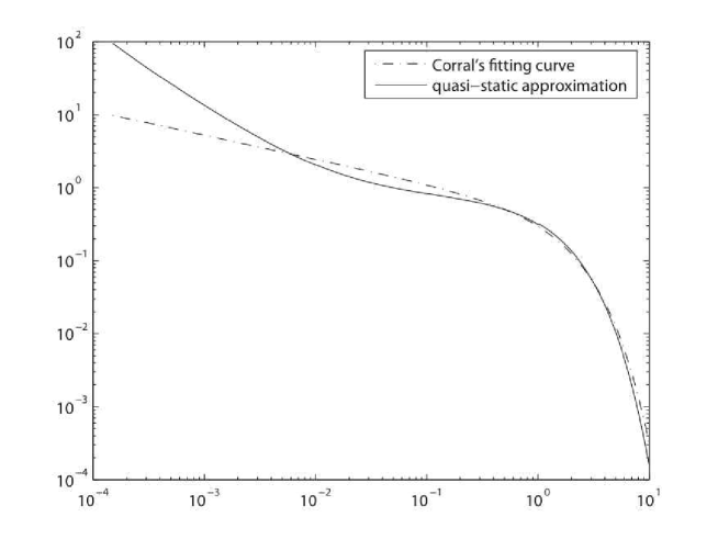
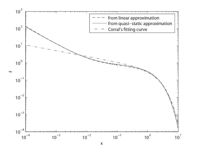
Fig. 1 reproduces the comparison obtained in Ref.SaichevSor06 ; SaichevSor07 between the function $f(x)$ given by (22) and Corral’s phenomenological functional fit Corral03 . Ref.SaichevSor06 ; SaichevSor07 found that expression (22) can fit rather well the empirical distributions of inter-event times, so as to even improve on Corral’s fit for short time scales, with $\alpha\approx 0.7-0.9$ and $n\approx 0.8-1.0$. These rather large intervals reflect a corresponding insensitivity of the quantitative shape of $f(x)$ with respect to $\alpha$ and $n$. An analysis of the impact of the first nonlinear term $\beta z^{\gamma}$ in the expansion (14) of $\Psi(z)$ in the nonlinear equations (10) and (11) led Saichev and Sornette to expect “weak departures from the results obtained with the linear approximation”. They added “It thus appears that the statistics of recurrence times is not sensitive enough to reveal the importance of these nonlinear corrections which describe the effect of cascades of generations of aftershocks.” It turns out that this statement was premature, as shown by our full treatment of the nonlinear equations. In particular, we identify significant biases in the estimation of the parameter $n$ when using the linear approximation. The reason lies in the fact that, for $\alpha$ close to $1$ (specifically $1\leq\gamma\leq 1.2$) as found in Ref.SaichevSor06 ; SaichevSor07 , the first nonlinear correction $\beta z^{\gamma}$ is only weakly nonlinear. We show below that the inclusion of the next term $\sim z^{2}$ changes somewhat the conclusions. In contrast, the higher-order terms beyond $z^{2}$ do not change the conclusions.

III Analysis of the full nonlinear equations (10) and (11)

III.1 Preparation of the equations and notations

Using the first four summands of the expansion (14), equations (10,11) can be written in the following form:

$$N_{-}(\tau,m_{d})=\frac{Q(m_{d})}{N_{-}(m_{d})}+\delta\Phi(\tau)\otimes N_{-}(\tau,m_{d})+\sigma N_{-}(m_{d})[\Phi(\tau)\otimes N_{-}(\tau,m_{d})]^{2},$$ (23)

$$\begin{array}[]{c}\displaystyle N(t,\tau,m_{d})=n[\Phi(t)\otimes N(t,\tau,m_{d})+\Phi(t+\tau)\otimes N_{-}(\tau,m_{d})]-\\ \displaystyle-\beta[\Phi(t)\otimes N(t,\tau,m_{d})+\Phi(t+\tau)\otimes N_{-}(\tau,m_{d})]^{\gamma}+\\ \displaystyle+\eta[\Phi(t)\otimes N(t,\tau,m_{d})+\Phi(t+\tau)\otimes N_{-}(\tau,m_{d})]^{2},\end{array}$$ (24)

where

$$\sigma=\eta[1-Q^{1-2/\gamma}(m_{d})].$$ (25)

In the present case, $N_{-}(m_{d})$ defined in (16) is not identical to $Q(m_{d})/(1-\delta)$ as in the linear approximation. Instead, $N_{-}(m_{d})$ is the root of a simple quadratic equation. However, the difference can be small: for instance, for $m_{d}-m_{0}=2,\theta=0.03,\gamma=1.2,n=0.9$, we have $Q(m_{d})/(1-\delta)\simeq 1.93*10^{-2}$ compared with $N_{-}(m_{d})\simeq 1.90*10^{-2}$.

Defining the dimensionless variables $x=\lambda t$, $y=\lambda\tau$ with $\lambda=\omega N_{-}(m_{d})$ and the functions

$$M_{-}(y)=N_{-}\left(\frac{y}{\lambda},m_{d}\right),\quad M(x,y)=N\left(\frac{x}{\lambda},\frac{y}{\lambda},m_{d}\right),$$ (26)

$$\Phi_{\epsilon}(x)=\lambda\Phi\left(\frac{x}{\lambda}\right).$$ (27)

the equations (23) and (24) become

$$M_{-}(y)=\frac{Q(m_{d})}{\lambda}+\delta\Phi_{\epsilon}(y)\otimes M_{-}(y)+\sigma\lambda[\Phi_{\epsilon}(y)\otimes M_{-}(y)]^{2},$$ (28)

$$\begin{array}[]{c}\displaystyle M(x,y)=n[\Phi_{\epsilon}(x)\otimes M(x,y)+\Phi_{\epsilon}(x+y)\otimes M_{-}(y)]-\\ \displaystyle-\beta[\Phi_{\epsilon}(x)\otimes M(x,y)+\Phi_{\epsilon}(x+y)\otimes M_{-}(y)]^{\gamma}+\\ \displaystyle+\eta[\Phi_{\epsilon}(x)\otimes M(x,y)+\Phi_{\epsilon}(x+y)\otimes M_{-}(y)]^{2}~{}.\end{array}$$ (29)

For the numerical calculations, we transform equation (28) into an equation for the new function $g(y)=1-M_{-}(y)/\lambda$:

$$\begin{array}[]{c}\displaystyle g(y)=1-\delta-\frac{Q(m_{d})}{\lambda}+\delta\left[a_{\epsilon}(y)+\Phi_{\epsilon}(y)\otimes g(y)\right]-\\ \displaystyle-\sigma\lambda\left[a_{\epsilon}(y)+\Phi_{\epsilon}(y)\otimes g(y)-1\right]^{2},\quad a_{\epsilon}(y)=\int\limits_{x}^{\infty}\Phi_{\epsilon}(x^{\prime})dx^{\prime}~{}.\end{array}$$ (30)

Solving for $g(y)$ instead of $M_{-}(y)$ is more efficient numerically because $g(y)$ is a monotonically decreasing function unlike $M_{-}(y)$. This ensures a faster numerical convergence and a weaker sensitivity to the finite mesh size of the discretization scheme. Equations (29) and (30) form the basis for our numerical calculations.

III.2 Numerical solution

The first step is to solve (30) for the function $g(y)$ that we reformulate as equation (34) given in the Appendix A. we use the method of successive approximations to obtain the value of the function $g(y_{i})$ on a regular grid $y_{i}=y_{0}+i\cdot dy$ with a small mesh $dy$. The performance of this method is discussed in Appendix A in the context of the linear approximation.

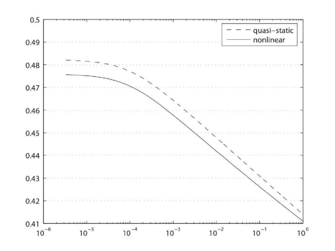
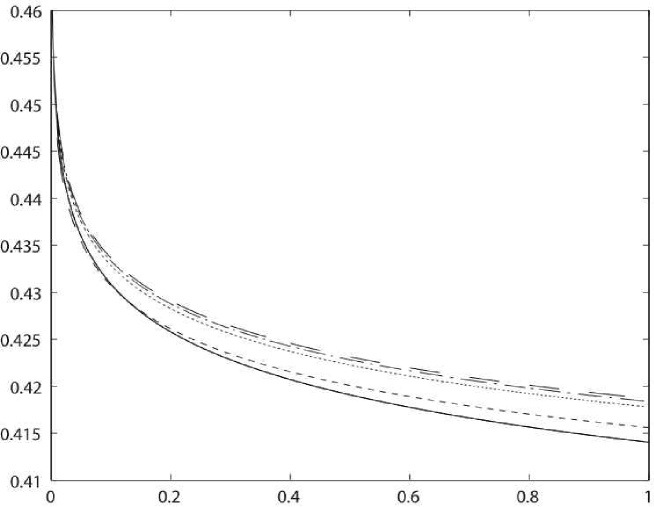
Fig.2 shows the difference between the quasi-static approximation (19) and the solution of the nonlinear equation (30). One can observe that the nonlinear solution lies under the quasi-static approximation, i.e., it gives a correction which is in the opposite direction compared with the linear solution (see fig.3 ).

The next step is to determine the function $M(x,y)$, obtained as the solution of equation (29). Note that the convolution operation involving $M_{-}(y)$ can now be expressed in terms of the known function $g(y)$:

$$\Phi_{\epsilon}(x+y)\otimes M_{-}(y)=a_{\epsilon}(t)-a_{\epsilon}(t+\tau)-\Phi_{\epsilon}(x+y)\otimes g(y)~{}.$$ (31)

In the nonlinear case, the function $M(x,y)$ cannot be represented analytically through the function $M_{-}(y)$ as in the linear case. This means that we have to calculate $M(x,y)$, a function of two variables (which significantly slows down the calculation speed). Equation (31) implies that the functions $\Phi_{\epsilon}(x+y)$ and $g(y)$ should be estimated on the same grid points $(x+y)_{k}$ and $y_{l}$. Therefore, the mesh sizes of $x$ and of $y$ should be identical: $dx=dy$.

In order to determine the probability $P(\tau)=\varphi(y,m_{d})$, we must also estimate the integral

$$\int\limits_{0}^{\infty}M(x,y)dy~{}.$$ (32)

This requires to span a large set of $y$ values in order to approximate the theoretical one $[0;+\infty]$ which, together with the condition $dx=dy$, make the problem very demanding in memory capacity. For example, for $x\in[0;1]$ and $y\in[0;1]$ with $dy=dx\sim 10^{-4}$, $M(x,y)$ is a matrix with $10^{8}$ elements. To alleviate this burden on memory capacity, we divide the $y$-interval into smaller intervals $y_{n},n=1,2,...,N$ and we determine the matrix $M(x,y_{n})$ consecutively for each of these sub-intervals. Having determined the probability function $\varphi(y,m_{d})$ on each such small intervals $y_{n}$, we use a simple smoothing polynomial interpolating scheme in order to prevent jumps in its second order derivative.

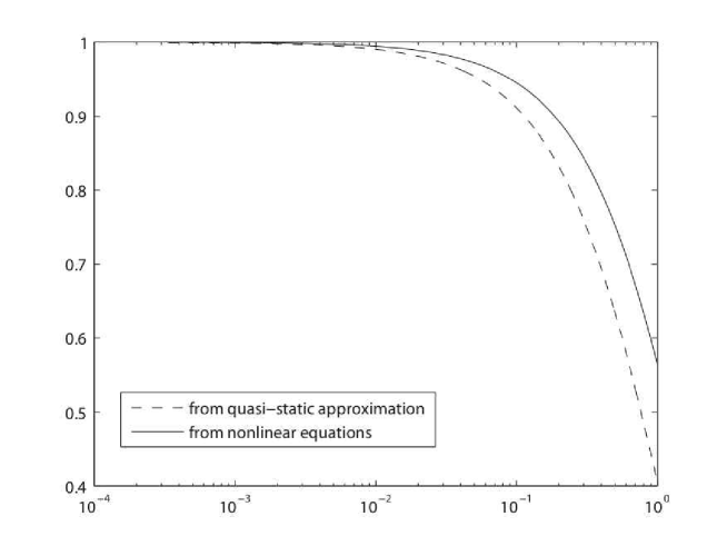
An example of the resulting probability $P(y)$ defined in (9) is shown in fig. 4, which identifies a significant difference between the quasi-static approximation presented in Ref. SaichevSor06 ; SaichevSor07 and the nonlinear solution.

III.3 Comparison between the linear and nonlinear versions of the theory and direct ETAS simulated catalogs

We present a comparison for the pdf of inter-event times obtained with

1. the linear analytic quasi-static approximation,

2. the numerical solution of the nonlinear equations (29) and (30) and

3. “exact” synthetic catalogs.

The two former solutions are obtained by taking the second order derivative of the functions $P(y)$ ($\varphi(y,m)$) shown in fig. 4, according to (21). The synthetic catalog was obtained using the method described in Appendix B. The ETAS parameters used here are: $n=0.9,\theta=0.05,\gamma=1.1,m_{d}-m_{0}=0$.

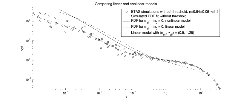
Fig. 5 shows the three pdf’s obtained by the three methods. For the “exact” pdf reconstructed from a synthetic ETAS catalog, we show both the histogram and a fit using a function constructed as the ratio between a polynomial function of order $5$ divided by another polynomial function of order $4$. These functions are expressed in terms of the logarithm of the dimensionless inter-event time. This fit has no pretence of rigor, it only provides a useful guide to the eye.

Fig.5 shows that the linear theory is significantly in error while the nonlinear theory provides an excellent agreement with the “exact” pdf for values of the dimensionless time interval $x\geq 4\cdot 10^{-2}$. For smaller $x$’s, the difference is due to numerical errors in the treatment of equations (29) and (30), which can be removed by using an adaptive mesh size, as discussed shortly below. The discrepancy between the “exact” pdf and the one obtained using the linear approximation implies that a fit of empirical pdf’s using the linear theory will likely provide spurious values for the significant parameters $n$ and $\gamma$. Indeed, a good fit of the “exact” synthetic pdf shown in fig.5 is obtained with the linear theory using effective parameters $n_{\rm eff}=0.86$ and $\gamma_{\rm eff}=1.28$, showing here a systematic bias of $5\%$ in the determination of $n$ and over $16\%$ in the determination of $\gamma$ (and therefore of the productivity $\alpha$).

Let us now return to the discrepancy between the nonlinear theory and the “exact” pdf observed for $x<4\cdot 10^{-2}$ in fig.5. Two possible factors need to be discussed:

1. impact of terms of order higher than $z^{2}$ in the expansion (14) of the function $\Psi(z)$ given by (13);

2. lack of convergence of the numerical scheme to solve equations (29) and (30), due to a too large mesh size.

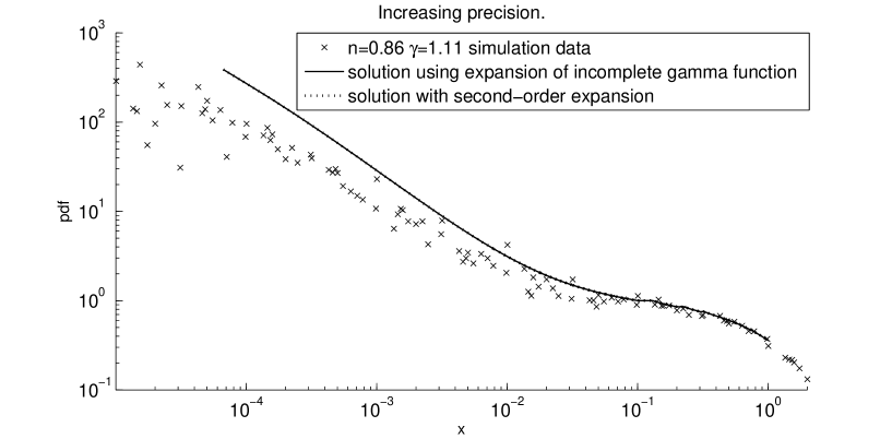
Fig. 6 rules out the first explanation, since the solution of the nonlinear equations obtained by using the full expression (13) in the calculation of equation (29) is undistinguishable from the solution obtained with the expansion (14). This check and other tests confirm that there is no need to complicate the computations by adding the calculation of the incomplete gamma function. This is important when using our theory for inverting the parameters from fits to empirical data, for instance.

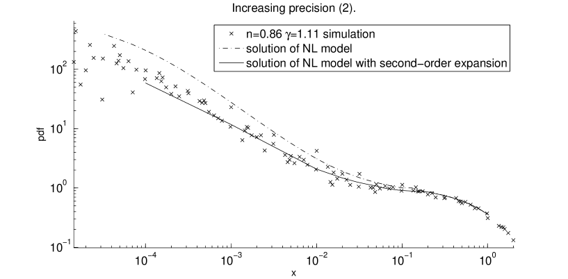
With respect to the second factor, we improve the numerical precision by varying the mesh size $dx$ so that $dx/x$ remains approximately equal to $10^{-4}$ for $x<0.1$ while $dx$ is fixed at $10^{-4}$ for $x\geq 0.1$. Thus, for $x\simeq 0.001$, we have chosen $dx\simeq 10^{-7}$, which is the limit that we have been able handle due to limited numerical precision of the computer. Fig 7 shows for the example $n=0.86,\theta=0.05,\gamma=1.11$ that the problem previously noted in fig. 5 disappears: there is a good agreement between the “exact” pdf obtained from the synthetic ETAS catalog and the nonlinear theory down to $x=0.001$.

III.4 Test of the inversion of the parameters $n$ and $\gamma$ using the nonlinear theory from a synthetic ETAS catalog

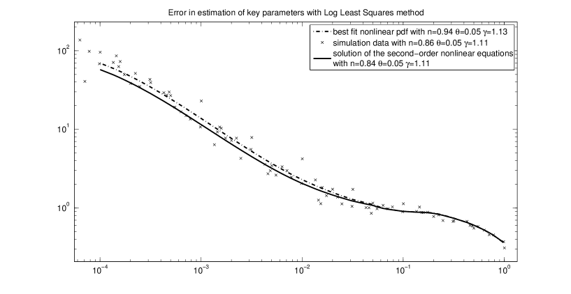
Consider a synthetic ETAS catalog of inter-event times for some fixed values of the parameters $n_{\rm cat},\theta_{\rm cat},\gamma_{\rm cat}$ and $\{m_{d}-m_{0}\}_{\rm cat}$. In this example, we take specifically $n_{\rm cat}=0.86,\theta_{\rm cat}=0.05,\gamma_{\rm cat}=1.11$ and $\{m_{d}-m_{0}\}_{\rm cat}=0$. Figure 8 shows the “exact” pdf of inter-event times (crosses), which mimics a real-life situation with statistical fluctuations. In a real-life experiment, one would like to use the nonlinear theory to invert for the unknown parameters $n,\theta,\gamma,m_{d}-m_{0}$. In this goal, using the nonlinear theory, we calculate the predicted pdf $f_{\rm NL}(x)$ of inter-event times for fixed values of the parameters $n,\theta,\gamma$ and $m_{d}-m_{0}$. For a given set of these four parameters, we construct the mean-square error of the logarithm of the pdf over the $N$ inter-event times of the catalog:

$$LLS(n,\theta,\gamma,m_{d}-m_{0})=\sum_{i=1}^{N}\left(\ln f_{\rm NL}(x_{i})-\ln f_{\rm cat}(x_{i})\right)^{2}~{},$$ (33)

where $f_{\rm NL}(x_{i})$ is the predicted pdf at the dimensionless inter-event time $x_{i}$ given by the nonlinear theory and $f_{\rm cat}(x_{i})$ is the corresponding empirical pdf (in the synthetic catalog). $LLS(n,\theta,\gamma,m_{d}-m_{0})$ quantifies how well the nonlinear prediction for the pdf of inter-event times can describe the (synthetic) data. The unknown parameters $n,\theta,\gamma,m_{d}-m_{0}$ are then obtained by finding the quadruplets which makes $LLS(n,\theta,\gamma,m_{d}-m_{0})$ minimum.

In practice, given the computational cost of the numerical solution of the nonlinear theory, we have found unpractical to explore systematically the four dimensional parameter space (with super-computer resources, this is not excluded but the next section removes the motivation to explore further this option as we will see). For the sake of demonstration, we assume that we already know $\theta=\theta_{\rm cat}=0.05$ and $m_{d}-m_{0}=\{m_{d}-m_{0}\}_{\rm cat}=0$. We are then left with searching for the remaining parameters $n$ and $\gamma$. For this, we form a grid in the $(n,\gamma)$ plane over which we find the minimum of $LLS(n,\gamma;\theta_{\rm cat},\theta_{\rm cat})$. The corresponding inverted values are $n_{\rm best~{}fit}=0.94\pm 0.02$ and $\gamma_{\rm best~{}fit}=1.13\pm 0.02$. The recovery of $\gamma$ (and therefore of the productivity exponent $\alpha$) is good, while there is $9\%$ error on $n$. Figure 8 shows that this best pdf fits well the “exact” pdf obtained from the ETAS catalog and is not far from the pdf predicted by the nonlinear theory with the true parameters.

IV On the lack of power of the pdf of inter-event times to invert for the clustering parameter $n$ and other parameters

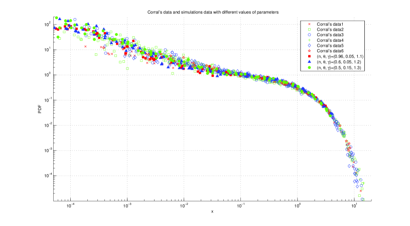
The title of this section is motivated by fig.9 comparing the pdf of inter-event times in synthetic ETAS catalogs with three different sets of parameters and the pdf’s obtained by Corral in different regions of the world Corral03 .

First, one can observe that the three triplets $(n=0.96,\theta=0.05,\gamma=1.1)$, $(n=0.6,\theta=0.05,\gamma=1.2)$ and $(n=0.5,\theta=0.15,\gamma=1.1)$ give almost the same pdf’s over the whole range of dimensionless inter-event times $10^{-4}\leq x\leq 15$. For $x>0.1$, the data collapse is almost perfect, while the scatter is larger for the smaller $x$ values. This is bad news for the determination of the clustering parameter $n$ in particular, since relatively small changes in the Omori law parameter $\theta$ and in the productivity law parameter $\gamma$ can compensate for a quite significant change in the branching ratio $n$. This suggests that previous claims on the use of the pdf of inter-event times to extract efficiently the clustering parameter have been over-optimistic Hainzl2006 ; Hardebeck07 .

Second, fig.9 shows that the three chosen triplets of parameters are basically equally good at fitting Corral’s data sets Corral03 . We note that, again for $x>0.1$, all empirical data and ETAS simulations present an almost perfect collapse on a quasi-universal curve. Larger scatter characterize smaller $x$ values, which is the region to scrutinize in the hope of extracting some useful constraints on the parameter values.

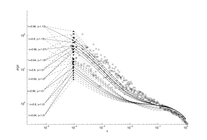
Actually, the situation is even more involved since, in addition to the parameters $n,\theta$ and $\gamma$, a genuine inversion needs also to determine $m_{d}-m_{0}$ (whose impact is significant as shown in Ref. SorWerner05 ) as well as the regularizing constant $c$ in the Omori law (2). Fig. 10 presents the pdf’s calculated with the nonlinear theory for different sets of four of these parameters $(n,\gamma,m_{d}-m_{0},c)$ with a fixed $\theta=0.05$, together with Corral’s data. For the pdf’s obtained from the nonlinear theory, we used all combinations between the three values $n=0.64,0.8,0.96$, the three values $\gamma=1.01,1.07,1.13$, two values $m_{d}-m_{0}=0.1,1$ and two values $\epsilon(c)\equiv\lambda c=10^{-4},10^{-5}$, corresponding to a total of 36 combinations. One can observe roughly two clusters among these 36 theoretical curves. All curves with $\gamma=1.01$ belong to the lower cluster, which is clearly not fitting the data. The upper cluster, which is in better agreement with the data, corresponds to the larger values $\gamma=1.07$ and $1.13$. This suggests that the productivity parameter $\alpha$ is likely to be smaller than (instead of equal to) the $b$-value of the Gutenberg-Richter law (recall that $\gamma=b/\alpha$). There is also a smaller impact of $\epsilon$ and of $m_{d}-m_{0}$: in general, higher values of these parameters displace the pdf downward.

The comparison between these 36 theoretical pdf’s and Corral’s data in figure 10 shows that there are large uncertainties in the inversion of the parameters. One could argue that the parameter $\theta$ should perhaps be modified to a value different from $0.05$ in order to better describe the data for small $x$’s. But this region is very sensitive to errors such as resulting from incompleteness HelmKJ ; Kagan03 and its use is problematic.

V Conclusion

We can conclude by the following rather conservative assessment. Recalling the definition of the dimensionless variable $x=\lambda\tau$, where $\lambda$ is the average seismicity rate of a given region and $\tau$ is a realization of the random variable defined as the inter-event time between two successive events in that region, we observe on the one-hand that the range of dimensionless inter-event times $x\geq 0.1$ is probably quite reliable from an empirical view point but the corresponding pdf’s are remarkably insensitive to the specific values of the clustering parameter, Omori law exponent, productivity exponent and completeness of the catalogs. On the other hand, the range of $x<0.1$ which would promise to give more sensitivity is not only highly unreliable but also lacks significant power to obtain a good inversion due to the existence of many almost equally good fits with quite different sets of parameters. Our theoretical analysis and its comparison with Corral’s data does not seem to support the proposition that inter-event time distributions could provide a new and more reliable way to measure of the so-called background earthquake activity as suggested in Ref.Hainzl2006 ; Hardebeck07 .

Acknowledgements: We are grateful to A. Corral for sharing his data with us.

Appendix A: Numerical solution for the linear approximation

This appendix provides a validation step of the numerical discretization scheme that we have developed to solve the nonlinear equations (29) and (30). Here, we apply this scheme to the linear approximation and compare the result with those which are available analytically. In the linear case, the equation (30) for $g(y)$ reduces to the following implicit linear integral equation

$$g(y)=\delta[a_{\epsilon}(y)+\Phi_{\epsilon}(y)\otimes g(y)]~{},$$ (34)

where $\delta$ is defined in (17). To solve (34), we use the method of successive approximations to obtain the value of the function $g(y_{i})$ on a regular grid $y_{i}=y_{0}+i\cdot dy$ with a small mesh $dy$. This method is adapted to the treatment of the convolution integral in the right-hand-side of (34). This simple method is fast and provides good convergence. For example, with $dy\sim 10^{-4}$, the calculation converges on the 15-th iteration with a residual absolute error $\sim 10^{-15}$.

This is illustrated in Fig. 11 which shows the function $g(y)$ in the linear approximation, obtained directly from the numerical solution of equation (34) for $dy=10^{-5}$ and $10^{-4}$, and by using the equation for $M_{-}(y)$ for $dy=10^{-5}$ and $10^{-4}$. As mentioned in the main text, the convergence is faster when using $g(y)$ compared with using $M_{-}(y)$. Eventually, as the mesh size goes to zero, both methods converge towards the same estimation. An illustration of this convergence is given with $dy=10^{-5}$, which shows much better agreement between the two estimations compared with the results obtained for $dy=10^{-4}$. The function $g(y)$ obtained by solving (34) is almost identical for $dy=10^{-5}$ and $10^{-4}$, demonstrating the faster convergence of this scheme. Fig. 11 also shows that the quasi-static approximation is not perfect, but exhibits a relative error of about no more than $1\%$ in this example. Once $g(y)$ has been obtained, the distribution of inter-event times is obtained from equation (18), which can be expressed here as

$$\varphi(y,m_{d})=\exp\left(-\frac{1-n}{1-\delta}y-\frac{1-n}{\delta}\Delta\int\limits_{0}^{y}g(x)dx\right)~{},$$ (35)

and with (21). Using the function $g(y)$ obtained by solving (34) with $dy=10^{-5}$ gives the dimensionless pdf of inter-event times shown in Fig. 11. For comparison is also shown the pdf obtained by Saichev and Sornette with the quasi-static approximation SaichevSor06 ; SaichevSor07 . There is an excellent agreement between the two methods.

Appendix B: ETAS simulations

This appendix describes how we construct the pdf of inter-event times in specific synthetic catalogs generated with the ETAS model. Actually, we do not generate synthetic catalogs. Instead, we use the analytical form of the cumulative distribution function (cdf) $F_{k+1}(\tau)$ of the waiting time $\tau$ between the $k$-th and the $(k+1)$-th event, knowing the times and magnitudes of the preceding $k$ events, to draw the occurrence time of this $(k+1)$-th event. Generating in this way 1000 or more inter-event times, we use logarithmic bins to construct the histogram of these inter-event times. This construction provides the “true” or “exact” numerical benchmark against which to compare our theory and the empirical data.

The cdf $F_{k+1}(\tau)$ is obtained by recurrence as follows. For the first event, $F_{1}(\tau)$ is nothing but the cumulative probability of occurrence of a spontaneous (background) shock since the origin of time, given by definition by the Poisson law with rate $\omega$:

$$F_{1}(\tau)=1-e^{-\omega\tau}.$$ (36)

The cdf $F_{2}(\tau)$ of the waiting time from the first to the second shock is made of two contributions: (i) the second shock may again be a background event or (ii) it may be triggered by the first shock. This yields

$$F_{2}(\tau)=1-e^{-\omega\tau}e^{-\rho_{1}(1-a(\tau))}~{},$$ (37)

where $\rho_{1}=\rho(m_{1})$ is the productivity of the first shock obtained from expression (3) given its magnitude $m_{1}$, and $a(\tau)$ is defined in (20).

All following shocks are similarly either a background event or triggered by one of the preceding events. The cdf $F_{3}(\tau)$ of the waiting time between the second and the third shocks is thus given by

$$F_{3}(\tau)=1-e^{-\omega\tau}e^{-\rho_{1}(a(\tau_{2})-a(\tau_{2}+\tau))-\rho_{2}(1-a(\tau))}~{},$$ (38)

where $\tau_{2}$ is the realized time interval between the first and the second shocks. Iterating, we obtain the cdf $F_{k}(\tau)$ for the waiting between the $(k-1)$-th and $k$-th shocks under the following form

$$F_{k}(\tau)=1-e^{-\omega\tau}\exp\left[-\sum_{i=1}^{k-1}\rho_{k-i}\cdot\left(a\left(\sum_{j=2}^{i}\tau_{j}\right)-a\left(\sum_{j=2}^{i}\tau_{j}+\tau\right)\right)\right]~{},$$ (39)

where $\tau_{j}$ is the waiting time between the $(j-1)$-th event and the $j$-th event, and $\rho_{i}=\rho(m_{i})$ is the productivity of the $i$-th shock obtained from expression (3) given its magnitude $m_{i}$.

In order to generate the $(k+1)$-th inter-event time interval between the occurrence of the $k$-th and $(k+1)$-th shock, it is necessary to know the $k$ previous inter-events times between the $k$ previous shocks and their $k$ magnitudes. Since, in the ETAS model, the magnitudes are drawn independently according to the Gutenberg-Richter distribution (1), they can be generated once for all. In order to generate a catalog of $N$ events, we thus draw $N$ magnitudes from the law (1). In order to generate the corresponding $N$ inter-event times, we use the expression (39) iteratively from $k=1$ to $k=N$ in a standard way: since any cdf $F(x)$ of a random variable $x$ is by construction itself uniformly distributed in $[0,1]$, we obtain a given realization $x*$ of the random variable $x$ by drawing a random number $r$ uniformly in $[0,1]$ and by solving the equation $F(x*)=r$. In our case, we generate $N$ independent uniformly distributed random numbers $x_{1},...,x_{N}$ in $[0,1]$ and determine each $\tau_{i}$ successively as the solution of $F_{i}(\tau_{i})=x_{i}$.

Figure 1: Non-dimensional probability density function $f(x)$ of inter-events times for $m_{d}-m_{0}=2,\gamma=1.2,n=0.9,\theta=0.03$ (continuous line) compared with Corral’s phenomenological expression Corral03 (dashed-dotted line).

Figure 2: Solution $g(y)$ of the nonlinear equation (30) (continuous line) and quasi-static approximation (19) (dashed line). The parameters of the ETAS model are $m_{d}-m_{0}=2,\gamma=1.2,n=0.9,\theta=0.03$.

Figure 3: Function $g(y)$ obtained with different schemes: (solid) - quasi-static approximation developed in SaichevSor06 ; SaichevSor07 ; numerical solution of equation (34) for (dash-dotted) $dy=10^{-5}$ and (long dashed) - $10^{-4}$; numerical of solution of (28) for $M_{-}(y)$ yielding $g(y)=1-M_{-}(y)$: (dotted) $dy=10^{-5}$ and (dashed) $10^{-4}$. The ETAS parameters are $m_{d}-m_{0}=2,\gamma=1.2,n=0.9,\theta=0.03$.

Figure 4: Probability $P(y)$ defined in (9) obtained by the numerical solution of the nonlinear equations (29) and (30) (continuous line) compared with the quasi-static approximation reported in Ref. SaichevSor06 ; SaichevSor07 (dashed line). The ETAS parameters are $m_{d}-m_{0}=2,\gamma=1.2,n=0.9,\theta=0.03$.

Figure 5: Pdf of dimensionless inter-event times for the ETAS parameters equal to $n=0.9,\theta=0.05,\gamma=1.1,m_{d}-m_{0}=0$. The pdf obtained with the nonlinear theory leading to the equations (29) and (30) is shown with the solid line. The pdf obtained with the linear theory is shown as the dashed line. The “exact” pdf obtained by the simulation method described in Appendix B is shown in histogram form (circles) and with a smoothing fit (dashed-dotted) performed with a function defined as the ratio of a polynomial function of $5$-th order over another polynomial function of $4$-th order, in terms of the logarithm of the dimensionless inter-event times. The dotted line shows the pdf obtained with the linear theory with effective parameters $n_{\rm eff}=0.86$ and $\gamma_{\rm eff}=1.28$, chosen to fit the “exact” pdf in the region $x\geq 4\cdot 10^{-2}$ where the nonlinear theory is performing well.

Figure 6: Test showing that using the exact values of the incomplete gamma function (13) in the calculation of equation (29) is undistinguishable from the solution obtained with the expansion (14) which includes all four terms up to second-order.

Figure 7: Comparison between the “exact” pdf obtained from a synthetic ETAS catalog (crosses) with $n=0.86,\theta=0.05,\gamma=1.11$ and the nonlinear theory without (dashed line) and with (continuous line) adaptive mesh grid size as described in the text.

Figure 8: Comparison between (i) the “exact” pdf of inter-event times (crosses) generated with the ETAS model according to the method described in Appendix B with $n_{\rm cat}=0.86,\theta_{\rm cat}=0.05,\gamma_{\rm cat}=1.11$ and $\{m_{d}-m_{0}\}_{\rm cat}=0$, which mimics a real-life situation containing fluctuations, (ii) the best fit (dashed line) with the nonlinear theory and (iii) the pdf obtained with the nonlinear theory with the true values of the parameters (continuous line). For simplicity, we impose the true values $\theta=\theta_{\rm cat}=0.05$ and $m_{d}-m_{0}=\{m_{d}-m_{0}\}_{\rm cat}=0$ in the best fit and invert for the two other parameters, which yields $n_{\rm best~{}fit}=0.94\pm 0.02$ and $\gamma_{\rm best~{}fit}=1.13\pm 0.02$.

Figure 9: Comparison between the pdf’s of inter-event times in synthetic ETAS catalogs with three different sets of parameters and the pdf’s obtained by Corral in different regions of the world.

Figure 10: Comparison between the pdf’s obtained by Corral in different regions of the world and the 36 pdf’s of inter-event times calculated with the nonlinear theory for all combinations of the following sets (with a fixed $\theta=0.05$): $n=0.64,0.8,0.96$; (ii) $\gamma=1.01,1.07,1.13$; (iii) $m_{d}-m_{0}=0.1,1$; (iv) $\epsilon(c)=10^{-4},10^{-5}$. Solid lines: $m_{d}-m_{0}=0.1,\;c=10^{-4}$; dashed lines: $m_{d}-m_{0}=0.1,\;c=10^{-5}$; dashed-dotted lines: $m_{d}-m_{0}=1,\;c=10^{-4}$; dotted lines: $m_{d}-m_{0}=1,\;c=10^{-5}$.

Figure 11: Probability density functions (pdf) of inter-event times obtained by using the function $g(y)$ solution of (34) with $dy=10^{-5}$, with (35) and (21) (continuous line). The pdf obtained by Saichev and Sornette with the quasi-static approximation SaichevSor06 ; SaichevSor07 is shown as the dashed line. Corral’s fitting curve is the dotted-dashed line. The parameters of the ETAS model are $m_{d}-m_{0}=2,\gamma=1.2,n=0.9,\theta=0.03$.

References

- (1) Bak, P., K. Christensen, L. Danon, and T. Scanlon (2002), Phys. Rev. Lett., 88(17), 178501.
- (2) Barabási, A.-L., Nature 435, 207 (2005).
- (3) Corral, A., Phys. Rev. E 68, 035102(R) (2003).
- (4) Corral, A., Phys. Rev. Lett. 92, 108501 (2004).
- (5) Corral, A., Physica A, 340, 590-597 (2004).
- (6) Corral, A., Nonlinear Processes in Geophysics, 12, 89-100 (2005).
- (7) Corral, A., Phys. Rev. Lett., 95, 028501 (2005).
- (8) Corral, A., Phys. Rev. Lett., 97, 178501 (2006).
- (9) Corral, A., and K. Christensen, Phys. Rev. Lett., 96, 109801 (2006).
- (10) Crane, R. and D. Sornette, Searching with viral dynamics on social networks: Application to YouTube, working paper (2007).
- (11) Davidsen, J., and C. Goltz, Geophys. Res. Lett., 31, doi:10.1029/2004GL020892 (2004).
- (12) Davidsen, J., S. Stanchits and G. Dresen, Phys. Rev. Lett. 98, 125502 (2007).
- (13) Gao, J., Y. Cao, and J. Hu, Recurrence Time Distribution, Renyi Entropy, and Pattern Discovery, 2005 Conference on Information Sciences and Systems, The Johns Hopkins University, March 16 18, 2005.
- (14) Hainzl, S., F. Scherbaum, C. Beauval. Bulletin of the Seismological Society of America 96 (1), 313-320, (2006).
- (15) Hardebeck, J., Background seismicity rates from interevent-time statistics: spatial patterns appear stationary through time, working paper (2007).
- (16) Hawkes, A. G., Biometrika, 58(1), 83-90 (1971a).
- (17) Hawkes, A. G., J. Royal Stat. Soc. Series B (Meth.), 33(3), 438-443 (1971).
- (18) Hawkes, A. G., and D. Oakes, J. of Appl. Prob., 11(3), 493-503 (1974).
- (19) Helmstetter, A., Y. Y. Kagan, and D. D. Jackson, J. Geophys. Res., 110, B05S08, doi:10.1029/2004JB003286 (2005).
- (20) Helmstetter, A. and D. Sornette, J. Geophys. Res. 107, NO. B10, 2237, doi:10.1029/2001JB001580 (2002).
- (21) Helmstetter, A. and D. Sornette, Geophys. Res. Lett. 30 (11) doi:10.1029/2003GL017670 (2003).
- (22) Kagan, Y. Y., Pure and Appl. Geophys., 155, 537-573 (1999).
- (23) Kagan, Y.Y., Physics of the Earth and Planetary Inter. 135, 173-209 (2003).
- (24) Kagan, Y. Y., and L. Knopoff, J. Geophys. Res., 86 (B4), 2853-2862 (1981).
- (25) Lindman, M., K. Jonsdottir, R. Roberts, B. Lund, and R. Bdvarsson, Phys. Rev. Lett., 94, 108501 (2005).
- (26) Lindman, M., K. Jonsdottir, R. Roberts, B. Lund, and R. Bdvarsson, Phys. Rev. Lett., 96, 109802 (2006).
- (27) Livina, V. N., S. Havlin, and A. Bunde, Phys. Rev. Lett., 95, 208501 (2006).
- (28) Livina, V., S. Tuzov, S. Havlin and A. Bunde, Physica A 348, 591-595 (2005).
- (29) Molchan, G., Pure and Appl. Geophys., 162, 1135-1150 (2005).
- (30) Ogata, Y., J. Am. Stat. Assoc., 83, 9-27 (1988).
- (31) Pisarenko, V.F., A. Sornette, D. Sornette and M.V. Rodkin, New Approach to the Characterization of Mmax and of the Tail of the Distribution of Earthquake Magnitudes, in press in Pure and Applied Geophysics (2008) (http://arxiv.org/abs/physics/0703010)
- (32) Reasenberg, P., J. Geophys. Res. 90, 5479-5495 (2005).
- (33) Saichev, A. and D. Sornette, Phys. Rev. Letts. 97, 078501 (2006).
- (34) Saichev, A. and D. Sornette, J. Geophys. Res., 112, B04313, doi:10.1029/2006JB004536 (2007).
- (35) Sornette, D., F. Deschatres, T. Gilbert and Y. Ageon, Phys. Rev. Letts. 93 (22), 228701 (2004).
- (36) Sornette. D. and M.J. Werner, J. Geophys. Res., Vol. 110 (B9), B09303, 10.1029/2005JB003621 (2005).
- (37) Utsu, T., Y. Ogata, and R. S. Matsu’ura, J. Phys. Earth, 43, 1-33 (1995).
- (38) Vazquez, A., J. G. Oliveira, Z. Dezso, K. I. Goh, I. Kondor, and A. L. Barabasi, Physical Review E 73, 036127 (2006).
- (39) Zaslavsky, G.M. and M.K. Tippett, Phys. Rev. Lett. 67, 3251-3254 (1991).