OCU-PHYS 284

ITEP/TH-58/07


Boundary Ring or a

Way to Construct Approximate NG Solutions

with Polygon Boundary Conditions

II. Polygons Π¯¯Π\bar{\Pi}, which admit an inscribed circle


H.Itoyama and A.Morozov


Osaka City University, Japan

ITEP, Moscow, Russia


ABSTRACT


We further develop the formalism of arXiv:0712.0159 for approximate solution of Nambu-Goto (NG) equations with polygon conditions in AdS backgrounds, needed in modern studies of the string/gauge duality. Inscribed circle condition is preserved, which leaves only one unknown function y0(y1,y2)subscript𝑦0subscript𝑦1subscript𝑦2y_{0}(y_{1},y_{2}) to solve for, what considerably simplifies our presentation. The problem is to find a delicate balance – if not exact match – between two different structures: NG equation – a non-linear deformation of Laplace equation with solutions non-linearly deviating from holomorphic functions, – and the boundary ring, associated with polygons made from null segments in Minkovski space. We provide more details about the theory of these structures and suggest an extended class of functions to be used at the next stage of Alday-Maldacena program: evaluation of regularized NG actions.


1 Introduction

In this paper we begin consideration of the next class of approximate solutions to Nambu-Goto (NG) equations with null-polygon boundary conditions by the method suggested in [1]. This problem is important for the study of the string/gauge (AdS/CFT) duality [2, 3], reformulated recently [4]-[28] as an identity between regularized minimal areas in AdS5𝐴𝑑subscript𝑆5AdS_{5} and BDS/DHKS/BHT [29, 7, 8, 17] amplitudes for gluon scattering in N=4𝑁4N=4 SUSY YM. Unfortunately, even after this ground-breaking reformulation [4], explicit check of duality is escaping, even in the leading order of the strong-coupling expansion – as usual because of the technical difficulties on the stringy side. In this particular case the first hard problem is explicit solution to a special version of Plateau minimal-surface problem [30]: to Nambu-Goto equations in AdS5𝐴𝑑subscript𝑆5AdS_{5} geometry with the boundary conditions at the AdS𝐴𝑑𝑆AdS boundary, represented by a polygon ΠΠ\Pi with n𝑛n light-like (null) segments. We refer to [4] for explanation of how this polygon emerges in the problem after a sequence of transformations,

NGmodelσmodelTdualityala[31]σmodelNGmodel,formulae-sequenceNGmodel𝜎modelsuperscript𝑇duality𝑎𝑙𝑎[31]𝜎modelNGmodel{\rm NG\ model}\rightarrow\sigma-{\rm model}\ \ \stackrel{{\scriptstyle T-{\rm duality}\ a\ la\ \cite[cite]{[\@@bibref{}{KT}{}{}]}}}{{\longrightarrow}}\ \ \sigma-{\rm model}\rightarrow{\rm NG\ model},

and to [13, 23] for additional comments and notations. Irrespective of these motivations, the current formulation of the gauge/string duality is now made pure geometric, at least in the leading order:

regularized(areaofaminimalsurfaceinAdS5,boundedbyΠ)=regularized(ΠΠdyμdyμ(yy)2)regularizedareaofaminimalsurfacein𝐴𝑑subscript𝑆5boundedbyΠregularizedsubscriptcontour-integralΠsubscriptcontour-integralΠ𝑑superscript𝑦𝜇𝑑subscriptsuperscript𝑦𝜇superscript𝑦superscript𝑦2\displaystyle{\rm regularized}\ \Big{(}{\rm area\ of\ a\ minimal\ surface\ in}\ AdS_{5},\ {\rm bounded\ by}\ \Pi\Big{)}={\rm regularized}\left(\oint_{\Pi}\oint_{\Pi}\frac{dy^{\mu}dy^{\prime}_{\mu}}{(y-y^{\prime})^{2}}\right) (1.1)

and the first problem is to find what the minimal surface is (with problems of regularization and higher-order corrections arising at the next stage). As surveyed in [1], explicit solution to the first problem is currently available only for n4𝑛4n\leq 4 [32, 4] and the maximally symmetric case (Π=S1Πsuperscript𝑆1\Pi=S^{1}) at n=𝑛n=\infty. As usual with Plateau problem, even approximate methods are not immediately available beyond this exactly-solvable sector. In [1] an line-of-attack was suggested and the first approximate results obtained for the simplest Znsubscript𝑍𝑛Z_{n} configurations. The present paper describes the next step in the same direction, generalizing the results of [1] to the next non-trivial case: of polygons which do not have symmetry, but still have a restricted geometry, identified as “Π¯¯Π\bar{\Pi} possesses an inscribing circle” in [1]. In this case the boundary conditions and thus the solution are lying in AdS3𝐴𝑑subscript𝑆3AdS_{3} subspace of AdS5𝐴𝑑subscript𝑆5AdS_{5}, and the problem is reduced to finding a single non-trivial function, say y0(y1,y2)subscript𝑦0subscript𝑦1subscript𝑦2y_{0}(y_{1},y_{2}), while the other two are expressed through the AdS3𝐴𝑑subscript𝑆3AdS_{3} constraints [4],

y3=0(Y3=0)y02+1=y12+y22+r2(Y4=0)subscript𝑦30missing-subexpressionsubscript𝑌30superscriptsubscript𝑦021superscriptsubscript𝑦12superscriptsubscript𝑦22superscript𝑟2missing-subexpressionsubscript𝑌40\displaystyle\begin{array}[]{ccc}y_{3}=0&&(Y_{3}=0)\\ y_{0}^{2}+1=y_{1}^{2}+y_{2}^{2}+r^{2}&&(Y_{4}=0)\end{array} (1.4)

2 Approach to approximate solution: a summary of [1]

The strategy, suggested in [1] was to:

\bullet First, represent y0subscript𝑦0y_{0} as a power series,

y0=i,j0aijy1iy2jsubscript𝑦0subscript𝑖𝑗0subscript𝑎𝑖𝑗superscriptsubscript𝑦1𝑖superscriptsubscript𝑦2𝑗\displaystyle y_{0}=\sum_{i,j\geq 0}a_{ij}y_{1}^{i}y_{2}^{j} (2.1)

and rewrite NG equations in the form of recurrence relations for aijsubscript𝑎𝑖𝑗a_{ij}, with recursion relating the two adjacent ”levels” k=i+j𝑘𝑖𝑗k=i+j and leaving a number of free parameters. If the structure of the boundary ring is explicitly known, then expansion (2.1) can be modified in order to take boundary conditions into account from the very beginning, though this can cause additional convergency problems for the series.

\bullet Second, truncate the series at some level N𝑁N and specify the remaining free parameters which match the boundary conditions in the best possible way at given truncation level. Increasing N𝑁N provides better and better fit to both the NG equations and boundary conditions.

\bullet Fitting criteria and thus the resulting approximations can be different, depending on the further application. As explained in [1], one can improve either local or global approximation to boundary conditions or instead try to better match the behavior at the angles of the polygon, which is responsible for the main IR divergence of the regularized area of the minimal surface.

2.1 Recurrent relations and free parameters

The first recurrence relations were already found in [1]:

There are no relations at levels zero and two: all the corresponding coefficients, a00subscript𝑎00a_{00} and a10,a01subscript𝑎10subscript𝑎01a_{10},a_{01} are free parameters, i.e. there are ν0=1subscript𝜈01\nu_{0}=1 and ν1=0subscript𝜈10\nu_{1}=0 of them.

At level two NG equations impose a single relation:111 As clear already from this formula the choice of ak0subscript𝑎𝑘0a_{k0} and a0ksubscript𝑎0𝑘a_{0k} (instead of, say, ak0subscript𝑎𝑘0a_{k0} and ak,k1subscript𝑎𝑘𝑘1a_{k,k-1}) makes the limit a10,a010subscript𝑎10subscript𝑎010a_{10},a_{01}\rightarrow 0 singular. Note that original solution of [4] is exactly of this kind: aij=δi1δj1subscript𝑎𝑖𝑗subscript𝛿𝑖1subscript𝛿𝑗1a_{ij}=\delta_{i1}\delta_{j1} and singularities are easily resolved for it.

a11=a02(1+a002a102)+a20(1+a002a012)a01a10=a02A10+a20A01a01a10subscript𝑎11subscript𝑎021superscriptsubscript𝑎002superscriptsubscript𝑎102subscript𝑎201superscriptsubscript𝑎002superscriptsubscript𝑎012subscript𝑎01subscript𝑎10subscript𝑎02subscript𝐴10subscript𝑎20subscript𝐴01subscript𝑎01subscript𝑎10\displaystyle a_{11}=-\frac{a_{02}(1+a_{00}^{2}-a_{10}^{2})+a_{20}(1+a_{00}^{2}-a_{01}^{2})}{a_{01}a_{10}}=-\frac{a_{02}A_{10}+a_{20}A_{01}}{a_{01}a_{10}} (2.2)

where A01=1+a002a012subscript𝐴011superscriptsubscript𝑎002superscriptsubscript𝑎012A_{01}=1+a_{00}^{2}-a_{01}^{2} and A10=1+a002a102subscript𝐴101superscriptsubscript𝑎002superscriptsubscript𝑎102A_{10}=1+a_{00}^{2}-a_{10}^{2}. Next formulas involve a generalization of these quantities:

Akl=1+a002ka102la012subscript𝐴𝑘𝑙1superscriptsubscript𝑎002𝑘superscriptsubscript𝑎102𝑙superscriptsubscript𝑎012\displaystyle A_{kl}=1+a_{00}^{2}-ka_{10}^{2}-la_{01}^{2} (2.3)

At level three we get two relations:

a12=6a03a013a102A103a30a012a10A012a012a102(a1124a02a20)A03+a00a012(a02(A10A21+4a012a102)+a20A01A41)a012a10(A01A104a012a102),subscript𝑎126subscript𝑎03superscriptsubscript𝑎013superscriptsubscript𝑎102subscript𝐴103subscript𝑎30superscriptsubscript𝑎012subscript𝑎10superscriptsubscript𝐴012superscriptsubscript𝑎012superscriptsubscript𝑎102superscriptsubscript𝑎1124subscript𝑎02subscript𝑎20subscript𝐴03subscript𝑎00superscriptsubscript𝑎012subscript𝑎02subscript𝐴10subscript𝐴214superscriptsubscript𝑎012superscriptsubscript𝑎102subscript𝑎20subscript𝐴01subscript𝐴41superscriptsubscript𝑎012subscript𝑎10subscript𝐴01subscript𝐴104superscriptsubscript𝑎012superscriptsubscript𝑎102\displaystyle a_{12}=\frac{6a_{03}a_{01}^{3}a_{10}^{2}A_{10}-3a_{30}a_{01}^{2}a_{10}A_{01}^{2}-a_{01}^{2}a_{10}^{2}(a_{11}^{2}-4a_{02}a_{20})A_{03}+a_{00}a_{01}^{2}\big{(}a_{02}(A_{10}A_{21}+4a_{01}^{2}a_{10}^{2})+a_{20}A_{01}A_{41}\big{)}}{a_{01}^{2}a_{10}(A_{01}A_{10}-4a_{01}^{2}a_{10}^{2})},
a21=6a30a103a012A013a03a102a01A102a012a102(a1124a02a20)A30+a00a102(a20(A01A12+4a012a102)+a02A10A14)a01a102(A01A104a012a102)subscript𝑎216subscript𝑎30superscriptsubscript𝑎103superscriptsubscript𝑎012subscript𝐴013subscript𝑎03superscriptsubscript𝑎102subscript𝑎01superscriptsubscript𝐴102superscriptsubscript𝑎012superscriptsubscript𝑎102superscriptsubscript𝑎1124subscript𝑎02subscript𝑎20subscript𝐴30subscript𝑎00superscriptsubscript𝑎102subscript𝑎20subscript𝐴01subscript𝐴124superscriptsubscript𝑎012superscriptsubscript𝑎102subscript𝑎02subscript𝐴10subscript𝐴14subscript𝑎01superscriptsubscript𝑎102subscript𝐴01subscript𝐴104superscriptsubscript𝑎012superscriptsubscript𝑎102\displaystyle a_{21}=\frac{6a_{30}a_{10}^{3}a_{01}^{2}A_{01}-3a_{03}a_{10}^{2}a_{01}A_{10}^{2}-a_{01}^{2}a_{10}^{2}(a_{11}^{2}-4a_{02}a_{20})A_{30}+a_{00}a_{10}^{2}\big{(}a_{20}(A_{01}A_{12}+4a_{01}^{2}a_{10}^{2})+a_{02}A_{10}A_{14}\big{)}}{a_{01}a_{10}^{2}(A_{01}A_{10}-4a_{01}^{2}a_{10}^{2})}

and ν3=2subscript𝜈32\nu_{3}=2 free parameters a03subscript𝑎03a_{03} and a30subscript𝑎30a_{30}.

Similarly, at level k𝑘k there will be k1𝑘1k-1 relations imposed by NG equations, and νk=2subscript𝜈𝑘2\nu_{k}=2 out of k+1𝑘1k+1 coefficients ai,kisubscript𝑎𝑖𝑘𝑖a_{i,k-i} at this level will remain free. We always choose ak0subscript𝑎𝑘0a_{k0} and a0ksubscript𝑎0𝑘a_{0k} for these free parameters. They can be associated with two arbitrary functions – of y1subscript𝑦1y_{1} and y2subscript𝑦2y_{2} respectively, and this freedom resembles the general solution of the archetypical equation 2Yy1y2=0superscript2𝑌subscript𝑦1subscript𝑦20\frac{\partial^{2}Y}{\partial y_{1}\partial y_{2}}=0, given by Y(y1,y2)=f(y1)+g(y2)𝑌subscript𝑦1subscript𝑦2𝑓subscript𝑦1𝑔subscript𝑦2Y(y_{1},y_{2})=f(y_{1})+g(y_{2}) with two arbitrary functions f𝑓f and g𝑔g. We shall see in s.3 below that even more relevant can be analogy with the ordinary Laplace equation, solved by arbitrary holomorphic and antiholomorphic functions.

If series (2.1) is truncated at level N𝑁N, it contains (N+1)2superscript𝑁12(N+1)^{2} different coefficients aijsubscript𝑎𝑖𝑗a_{ij}, of which 2N+12𝑁12N+1 remain free parameters, unconstrained by NG equations.

2.2 Boundary conditions and the boundary ring

According to [1] the boundary conditions can be formulated in terms of the boundary ring ΠsubscriptΠ{\cal R}_{\Pi}, which consists of all polynomials of y𝑦y-variables that vanish on the boundary polygon ΠΠ\Pi.222 By definition, solutions of our problem belong to the intersection of the space of r=0𝑟0r=0 asymptotes of NG solutions with the completion of the boundary ring. In still other words, anzatze that we substitute into NG equations should be taken from completion of the boundary ring. Completion here means first, that, say, r2superscript𝑟2r^{2} rather than r𝑟r itself belongs to ΠsubscriptΠ{\cal R}_{\Pi} according to (1.4), i.e. r𝑟r belongs to the algebraic completion of the ring. Second, our anzatze can be looked for among formal series made out of elements of ΠsubscriptΠ{\cal R}_{\Pi}. Since y3=0subscript𝑦30y_{3}=0 this ΠsubscriptΠ{\cal R}_{\Pi} includes y3subscript𝑦3y_{3} as a generator and we can actually restrict considerations to polynomials, depending on only three variables y0,y1,y2subscript𝑦0subscript𝑦1subscript𝑦2y_{0},y_{1},y_{2}.

As further explained in [1], if n𝑛n edges of ΠΠ\Pi are defined by the equations:

{cay1+say2=ha,y0=y0a+σa(say1+cay2),casessubscript𝑐𝑎subscript𝑦1subscript𝑠𝑎subscript𝑦2subscript𝑎subscript𝑦0subscript𝑦0𝑎subscript𝜎𝑎subscript𝑠𝑎subscript𝑦1subscript𝑐𝑎subscript𝑦2\displaystyle\left\{\begin{array}[]{c}c_{a}y_{1}+s_{a}y_{2}=h_{a},\\ y_{0}=y_{0a}+\sigma_{a}(-s_{a}y_{1}+c_{a}y_{2}),\end{array}\right. (2.6)

with ca=cosϕasubscript𝑐𝑎subscriptitalic-ϕ𝑎c_{a}=\cos\phi_{a}, sa=sinϕasubscript𝑠𝑎subscriptitalic-ϕ𝑎s_{a}=\sin\phi_{a} and σa=±1subscript𝜎𝑎plus-or-minus1\sigma_{a}=\pm 1, see Fig.1, then

\bullet the condition that ΠΠ\Pi closes in y0subscript𝑦0y_{0} direction is

a=1nσala=0,superscriptsubscript𝑎1𝑛subscript𝜎𝑎subscript𝑙𝑎0\displaystyle\sum_{a=1}^{n}\sigma_{a}l_{a}=0, (2.7)

where lasubscript𝑙𝑎l_{a} are the lengths of Π¯¯Π\bar{\Pi}, which is projection of ΠΠ\Pi onto the (y1,y2)subscript𝑦1subscript𝑦2(y_{1},y_{2}) plane, and

\bullet the following three polynomials are the obvious elements of ΠsubscriptΠ{\cal R}_{\Pi}:

PΠ(y1,y2)=a=1n(cay1+say2ha),subscript𝑃Πsubscript𝑦1subscript𝑦2superscriptsubscriptproduct𝑎1𝑛subscript𝑐𝑎subscript𝑦1subscript𝑠𝑎subscript𝑦2subscript𝑎\displaystyle P_{\Pi}(y_{1},y_{2})=\prod_{a=1}^{n}\Big{(}c_{a}y_{1}+s_{a}y_{2}-h_{a}\Big{)},
P~Π(y0,y1)=a=1n(y1+()a+1sa(y0y0a)caha),subscript~𝑃Πsubscript𝑦0subscript𝑦1superscriptsubscriptproduct𝑎1𝑛subscript𝑦1superscript𝑎1subscript𝑠𝑎subscript𝑦0subscript𝑦0𝑎subscript𝑐𝑎subscript𝑎\displaystyle\tilde{P}_{\Pi}(y_{0},y_{1})=\prod_{a=1}^{n}\Big{(}y_{1}+(-)^{a+1}s_{a}(y_{0}-y_{0a})-c_{a}h_{a}\Big{)},
P~~Π(y0,y2)=a=1n(y2+()aca(y0y0a)saha)subscript~~𝑃Πsubscript𝑦0subscript𝑦2superscriptsubscriptproduct𝑎1𝑛subscript𝑦2superscript𝑎subscript𝑐𝑎subscript𝑦0subscript𝑦0𝑎subscript𝑠𝑎subscript𝑎\displaystyle\widetilde{\tilde{P}}_{\Pi}(y_{0},y_{2})=\prod_{a=1}^{n}\Big{(}y_{2}+(-)^{a}c_{a}(y_{0}-y_{0a})-s_{a}h_{a}\Big{)} (2.8)

Refer to caption
Refer to caption
Figure 1: Convention for labeling sides and vertices of the Znsubscript𝑍𝑛Z_{n}-symmetric polygon Π¯¯Π\bar{\Pi} (right). Its corresponding ΠΠ\Pi is shown in the left picture.

So far we imposed only one of the constraints (1.4), y3=0subscript𝑦30y_{3}=0. The second constraint can be imposed only if all ha=1subscript𝑎1h_{a}=1, and this is what we assume below in the present paper. As already stated, this condition implies the existence of a unit circle, inscribed into Π¯¯Π\bar{\Pi}. If additionally n𝑛n is even and σa=()asubscript𝜎𝑎superscript𝑎\sigma_{a}=(-)^{a}, then also all the n𝑛n parameters y0asubscript𝑦0𝑎y_{0a} coincide and we can put y0a=0subscript𝑦0𝑎0y_{0a}=0 by a constant shift of y0subscript𝑦0y_{0}: this choice corresponds to y0subscript𝑦0y_{0} vanishing at all points where the sides of Π¯¯Π\bar{\Pi} touch the inscribing circle.

2.3 Boundary conditions as sum rules

A possible way to describe above boundary conditions is also to write them down for each particular side of ΠΠ\Pi. On (2.6) we have (with ha=1subscript𝑎1h_{a}=1 and y0a=0subscript𝑦0𝑎0y_{0a}=0):

y1=casata,subscript𝑦1subscript𝑐𝑎subscript𝑠𝑎subscript𝑡𝑎\displaystyle y_{1}=c_{a}-s_{a}t_{a},
y2=sa+cata,subscript𝑦2subscript𝑠𝑎subscript𝑐𝑎subscript𝑡𝑎\displaystyle y_{2}=s_{a}+c_{a}t_{a},
y0=σatasubscript𝑦0subscript𝜎𝑎subscript𝑡𝑎\displaystyle y_{0}=\sigma_{a}t_{a} (2.9)

i.e.

z=y1+iy2=(ca+isa)(1+ita)=eiϕa(1+iσay0),𝑧subscript𝑦1𝑖subscript𝑦2subscript𝑐𝑎𝑖subscript𝑠𝑎1𝑖subscript𝑡𝑎superscript𝑒𝑖subscriptitalic-ϕ𝑎1𝑖subscript𝜎𝑎subscript𝑦0\displaystyle z=y_{1}+iy_{2}=(c_{a}+is_{a})(1+it_{a})=e^{i\phi_{a}}(1+i\sigma_{a}y_{0}), (2.10)

where tasubscript𝑡𝑎t_{a} is a parameter along the corresponding straight line. Along its segment, which is the side of ΠΠ\Pi it changes within some region ta[ta1,+ta2]subscript𝑡𝑎subscript𝑡𝑎1subscript𝑡𝑎2t_{a}\in[-t_{a1},+t_{a2}]. Then boundary conditions imply that

i,j0aij(casata)i(sa+cata)j=σata,ta[ta1,+ta2],a=1,,nformulae-sequencesubscript𝑖𝑗0subscript𝑎𝑖𝑗superscriptsubscript𝑐𝑎subscript𝑠𝑎subscript𝑡𝑎𝑖superscriptsubscript𝑠𝑎subscript𝑐𝑎subscript𝑡𝑎𝑗subscript𝜎𝑎subscript𝑡𝑎formulae-sequencesubscript𝑡𝑎subscript𝑡𝑎1subscript𝑡𝑎2𝑎1𝑛\displaystyle\sum_{i,j\geq 0}a_{ij}(c_{a}-s_{a}t_{a})^{i}(s_{a}+c_{a}t_{a})^{j}=\sigma_{a}t_{a},\ \ \ \ t_{a}\in[-t_{a1},+t_{a2}],\ \ \ a=1,\ldots,n (2.11)

A set of sum rules arise is we consider these equalities as term-by-term identities for series in powers of tasubscript𝑡𝑎t_{a}. For example, if coordinate system is rotated to put c1=1subscript𝑐11c_{1}=1, s1=0subscript𝑠10s_{1}=0, we get an infinite set of relations

j0aij=σ1δi1subscript𝑗0subscript𝑎𝑖𝑗subscript𝜎1subscript𝛿𝑖1\displaystyle\sum_{j\geq 0}a_{ij}=\sigma_{1}\delta_{i1} (2.12)

– to be supplemented by (n1)𝑛1(n-1) more similar sets, associated with other sides of ΠΠ\Pi. The free parameters ak0subscript𝑎𝑘0a_{k0} and a0ksubscript𝑎0𝑘a_{0k} are defined by boundary conditions.

Among other things, this consideration seems to imply that y0subscript𝑦0y_{0} should satisfy (2.6) along entire straight line, not only within the segment. This is consistent with the known property of solutions to Plateau problem in the flat Euclidean space [33].

2.4 Approximate methods

Unfortunately no way is known at the moment to solve above relations exactly, except for in a few simple situations, listed in s.2 of [1]. In order to proceed one is naturally turned to approximate considerations. However, there are no ready methods to address this kind of problems and one needs to practice the trial and error approach.

Usually approximation starts from making the best thinkable anzatz, explicitly taking into account all the already known properties of the problem (symmetries, to begin with) with remaining infinite-parameter freedom contained in adequately defined formal series. Then this anzatz is substituted into original equation, and – if the formal series was introduced in an adequate way (what is more a matter of art or lack than of a rigorous theory), – the equation turns into a recurrent relation for coefficients of the series. So far everything was exact, even if not fully deductive, approximation comes at the next stage: when infinite series is truncated at some level N𝑁N. Success of the method depends on the choice of ”original knowledge”, of particular anzatz, including a point to expand around and particular expansion parameters, and – not the least – on the properties of the problem, i.e. the very existence of effective truncations, producing reasonable approximation at sufficiently low N𝑁N.

In [1] various attempts were described to apply this procedure, and some of them seem relatively successful. The main problem appears to be a balance between reasonable introduction of formal series in local parameters (say, coordinates y𝑦y) consistent with differential nature of NG equations, and adequate imposition of global boundary conditions, relatively far from expansion point. It turns out that, somewhat unusually, the balance should better be shifted towards the boundary conditions.

2.5 The goal of this paper

Success of [1] was due to construction of specific polynomials, named 𝒫n(y0,y1,y2)subscript𝒫𝑛subscript𝑦0subscript𝑦1subscript𝑦2{\cal P}_{n}(y_{0},y_{1},y_{2}), which had four important properties:

\bullet 𝒫ΠΠsubscript𝒫ΠsubscriptΠ{\cal P}_{\Pi}\in{\cal R}_{\Pi} was an element of the boundary ring, thus an anzatz

𝒫Π=0subscript𝒫Π0\displaystyle{\cal P}_{\Pi}=0 (2.13)

satisfies boundary conditions exactly and it can be further generalized (perturbed) to

𝒫Π=P2subscript𝒫Πsubscript𝑃2\displaystyle{\cal P}_{\Pi}=P_{2}{\cal B} (2.14)

which continue to satisfy boundary conditions with any perturbation function (y0;y1,y2)subscript𝑦0subscript𝑦1subscript𝑦2{\cal B}(y_{0};y_{1},y_{2}).333 Additional Znsubscript𝑍𝑛Z_{n} symmetry, assumed in [1], allowed to put (y0;y1,y2)=y0B(y1,y2)subscript𝑦0subscript𝑦1subscript𝑦2subscript𝑦0𝐵subscript𝑦1subscript𝑦2{\cal B}(y_{0};y_{1},y_{2})=y_{0}B(y_{1},y_{2}), but this is not the case generically.

\bullet 𝒫nsubscript𝒫𝑛{\cal P}_{n} was linear in y0subscript𝑦0y_{0},

𝒫Π=y0QΠ(y1,y2)KΠ(y1,y2)subscript𝒫Πsubscript𝑦0subscript𝑄Πsubscript𝑦1subscript𝑦2subscript𝐾Πsubscript𝑦1subscript𝑦2\displaystyle{\cal P}_{\Pi}=y_{0}Q_{\Pi}(y_{1},y_{2})-K_{\Pi}(y_{1},y_{2}) (2.15)

what allowed to resolve (2.13) and treat it as an anzatz for a single-valued function

y0(0)(y1,y2)=KΠ(y1,y2)QΠ(y1,y2)superscriptsubscript𝑦00subscript𝑦1subscript𝑦2subscript𝐾Πsubscript𝑦1subscript𝑦2subscript𝑄Πsubscript𝑦1subscript𝑦2\displaystyle y_{0}^{(0)}(y_{1},y_{2})=\frac{K_{\Pi}(y_{1},y_{2})}{Q_{\Pi}(y_{1},y_{2})} (2.16)

After that (2.14) could be solved iteratively, a la [34], and provides a formal series perturbation of this function.

\bullet The polynomial QΠsubscript𝑄ΠQ_{\Pi} in (2.15) did not have zeroes inside Π¯¯Π\bar{\Pi}, in particular, it did not vanish at the origin,

QΠ(y1,y2)=1+O(y1,y2),subscript𝑄Πsubscript𝑦1subscript𝑦21𝑂subscript𝑦1subscript𝑦2\displaystyle Q_{\Pi}(y_{1},y_{2})=1+O(y_{1},y_{2}), (2.17)

what made the function (2.16) free of singularities, and this property was inherited by all perturbative corrections implied by (2.14).444 A little care is needed at this point if one wishes to include the y0subscript𝑦0y_{0}-linear terms from (y0,y1,y2)subscript𝑦0subscript𝑦1subscript𝑦2{\cal B}(y_{0},y_{1},y_{2}) into denominators of perturbation series, i.e. sum up the corresponding parts of the series exactly, what can always be done.

\bullet The polynomial KΠ(y1,y2)subscript𝐾Πsubscript𝑦1subscript𝑦2K_{\Pi}(y_{1},y_{2}) satisfied NG equations in the first approximation, i.e. application of NG operator provided only terms with higher powers of y1,y2subscript𝑦1subscript𝑦2y_{1},y_{2} than were present in KΠsubscript𝐾ΠK_{\Pi}. This property was easy to formulate in [1] because Znsubscript𝑍𝑛Z_{n}-symmetric KΠsubscript𝐾ΠK_{\Pi} considered there were homogeneous polynomials (of degree n/2𝑛2n/2), but it becomes a subtler concept in generic situation. Still it is this property that allows to honestly treat {\cal B} as a perturbation, needed to correct (2.16) in order to make it satisfying the NG equations.555 Note that this approach is somewhat unusual, because it shifts emphasize from differential equations to boundary conditions. Ref.[1] describes in length how this shift of accents occurs, here we use this modified view from the very beginning. Still, it deserves reminding that one of the reasons for it is that the modern opinion is that Plateau problem arises in string/gauge duality in a special context: we need minimal surfaces in AdS space with boundaries lying at its boarder (infinity or the origin, depending on parametrization of AdS), so that their areas are diverging near the boundary. What we need are regularized areas, but regularization requires exact knowledge of behavior at the boundary, i.e. of allowed type of asymptotics – in order to define physical quantities, which are independent of the coefficients in front of these asymptotical terms. This is what makes care about the boundary conditions the first priority. If they are taken into account in exact way, then one can always deal with equations a posteriori, by minimizing the resulting regularized area over remaining free parameters, which could otherwise be fixed a priori by exactly solving the original equations. As explained in [13], this approach can be much simpler and more practical.


Thus in this paper our primary goal is to search for an analogue of the polynomials 𝒫Πsubscript𝒫Π{\cal P}_{\Pi} in the case of generic ΠΠ\Pi with n𝑛n angles and inscribed circle in Π¯¯Π\bar{\Pi}. If they are constructed, then we can look at approximations to minimal surfaces provided by (2.16) and consider the actual role of corrections, which are obligatory non-vanishing, since =00{\cal B}=0 is inconsistent with NG equations. Actually, the present paper is only a step in this direction. We begin by constructing the theory from the very beginning, but leave many important branches of possible development only mentioned, what finally prevents us from providing an exhaustive answer. Thus de facto the goal is to describe the context, what opens a lot of room for improvements and for getting better and wider results.

2.6 Plan of the paper

Our first subject in s.3 is conversion of NG equations into recurrence relations. Such conversion can be made over different ”backgrounds”, the c𝑐c- and b𝑏b-series of [1] being particular examples. In s.3 we concentrate on the ”basic” example, with background zero, so that all other sets of recurrence relations can be considered as subalgebras of this main one. Our main interest here is deviation from harmonic functions due to the difference between non-linear NG operator and linear Laplace in one complex dimension – on the (y1,y2)subscript𝑦1subscript𝑦2(y_{1},y_{2}) plane.

The next s.4 addresses the problem of sharp angles – an important issue for applications in Alday-Maldacena program, because angles are the sources of most important quadratic divergencies of regularized actions. We explain how sharp-angle conditions can be formulated analytically. Of course, elements of the polygon boundary rings satisfy these conditions, but they are of course violated by generic solutions to NG equations, exact or approximate, before boundary conditions are imposed. Moreover, if boundary conditions are matched approximately, not exactly (like some options considered in [1]), one still has an opportunity to require that angles are sharp (not smoothened) – and it is here that these analytical formulas are especially useful.

In s.5 we address the problem of NG solutions for generic quadrilaterals. Despite it is solved in [13, 23], solution is not found in the form of explicit function y0(y1,y2)subscript𝑦0subscript𝑦1subscript𝑦2y_{0}(y_{1},y_{2}). A way to bring it to such form is provided by technique of non-linear algebra [35, 36]. We demonstrate that at n=4𝑛4n=4 this y0(y1,y2)subscript𝑦0subscript𝑦1subscript𝑦2y_{0}(y_{1},y_{2}) is always a solution to an explicit quadratic equation, like it turned out to be in the particular case of rhombi [1].

The following subject in s.6 is boundary rings for polygons ΠΠ\Pi. The main puzzle here is the structure behind the polynomials KΠsubscript𝐾ΠK_{\Pi} in eq.(2.15). In [1] they were obtained from somewhat mysterious manipulations with P𝑃P’s from (2.8) and were found to have a form, which is very similar to (2.8) in Znsubscript𝑍𝑛Z_{n}-symmetric situation with even n𝑛n:

Kn/2a=1n/2(say1+cay2)similar-tosubscript𝐾𝑛2superscriptsubscriptproduct𝑎1𝑛2subscript𝑠𝑎subscript𝑦1subscript𝑐𝑎subscript𝑦2\displaystyle K_{n/2}\sim\prod_{a=1}^{n/2}\Big{(}s_{a}y_{1}+c_{a}y_{2}\Big{)} (2.18)

The problem is that this time the product at the r.h.s. is only over a half of segments and thus can not be immediately generalized to asymmetric cases (going from even to odd n𝑛n introduces additional problem: the simplest choice of σa=()a1subscript𝜎𝑎superscript𝑎1\sigma_{a}=(-)^{a-1} can not be made). We demonstrate in s.6 how such polynomials can actually be constructed – though they probably do not play the same role as they did in [1]. The reason is that already in the first non-trivial asymmetric configuration – at n=4𝑛4n=4 – exact solution is associated with the boundary ring element, which is not linear, but quadratic in y0subscript𝑦0y_{0}, see s.2.6 of [1]. This is the first signal that the proper analogue of 𝒫Πsubscript𝒫Π{\cal P}_{\Pi} in asymmetric case should not be linear. At the same time, s.5 demonstrates that quadratic can be enough, at least at n=4𝑛4n=4 it is the case. It is still unclear what the situation is going to be beyond for n>4𝑛4n>4, where explicit solutions of NG equations are yet unknown. A promising option is to look for the adequate anzatze among the boundary ring elements of order n/2𝑛2n/2 in y0subscript𝑦0y_{0}. According to the strategy, outlined in [13] and [1] we suggest to parameterize potentially relevant elements of the boundary rings by a few parameters, and treat them as if they were moduli of NG solutions, i.e. evaluate the regularized action and minimize it w.r.t. these parameters. This approach can finally turn simpler then direct solution of NG equations by methods, considered in s.3.

Appendix at the end of the paper contains some remarks about sophisticated notations used throughout the text.

3 NG equations as recurrence relations

The first recurrence relations were already found in [1]. It will be more convenient to switch to the complex coordinates z=y1+iy2𝑧subscript𝑦1isubscript𝑦2z=y_{1}+{\rm i}y_{2}, z¯=y1iy2¯𝑧subscript𝑦1isubscript𝑦2\bar{z}=y_{1}-{\rm i}y_{2} in the (y1,y2)subscript𝑦1subscript𝑦2(y_{1},y_{2}) plane and write instead of (2.1)

y0=k,j0(αkjzk+α¯kjz¯k)(zz¯)j=k,j0Re(αkjzk)(zz¯)jsubscript𝑦0subscript𝑘𝑗0subscript𝛼𝑘𝑗superscript𝑧𝑘subscript¯𝛼𝑘𝑗superscript¯𝑧𝑘superscript𝑧¯𝑧𝑗subscript𝑘𝑗0Resubscript𝛼𝑘𝑗superscript𝑧𝑘superscript𝑧¯𝑧𝑗\displaystyle y_{0}=\sum_{k,j\geq 0}\left(\alpha_{kj}z^{k}+\bar{\alpha}_{kj}\bar{z}^{k}\right)(z\bar{z})^{j}=\sum_{k,j\geq 0}{\rm Re}\left(\alpha_{kj}z^{k}\right)(z\bar{z})^{j} (3.1)

3.1 Reduced NG action

Recurrent relations result from substitution of a formal series representation for y0(y1,y2)subscript𝑦0subscript𝑦1subscript𝑦2y_{0}(y_{1},y_{2}) into NG equations, which for y3=0subscript𝑦30y_{3}=0 have the form

y1(y0y1H22r2LNG)+y2(y0y2H11r2LNG)y1(y0y2H12r2LNG)y2(y0y1H12r2LNG)=0,subscript𝑦1subscript𝑦0subscript𝑦1subscript𝐻22superscript𝑟2subscript𝐿𝑁𝐺subscript𝑦2subscript𝑦0subscript𝑦2subscript𝐻11superscript𝑟2subscript𝐿𝑁𝐺subscript𝑦1subscript𝑦0subscript𝑦2subscript𝐻12superscript𝑟2subscript𝐿𝑁𝐺subscript𝑦2subscript𝑦0subscript𝑦1subscript𝐻12superscript𝑟2subscript𝐿𝑁𝐺0\displaystyle\frac{\partial}{\partial y_{1}}\left(\frac{\partial y_{0}}{\partial y_{1}}\frac{H_{22}}{r^{2}L_{NG}}\right)+\frac{\partial}{\partial y_{2}}\left(\frac{\partial y_{0}}{\partial y_{2}}\frac{H_{11}}{r^{2}L_{NG}}\right)-\frac{\partial}{\partial y_{1}}\left(\frac{\partial y_{0}}{\partial y_{2}}\frac{H_{12}}{r^{2}L_{NG}}\right)-\frac{\partial}{\partial y_{2}}\left(\frac{\partial y_{0}}{\partial y_{1}}\frac{H_{12}}{r^{2}L_{NG}}\right)=0,
y1(ry1H22r2LNG)+y2(ry2H11r2LNG)y1(ry2H12r2LNG)y2(ry1H12r2LNG)+2LNGr=0subscript𝑦1𝑟subscript𝑦1subscript𝐻22superscript𝑟2subscript𝐿𝑁𝐺subscript𝑦2𝑟subscript𝑦2subscript𝐻11superscript𝑟2subscript𝐿𝑁𝐺subscript𝑦1𝑟subscript𝑦2subscript𝐻12superscript𝑟2subscript𝐿𝑁𝐺subscript𝑦2𝑟subscript𝑦1subscript𝐻12superscript𝑟2subscript𝐿𝑁𝐺2subscript𝐿𝑁𝐺𝑟0\displaystyle\frac{\partial}{\partial y_{1}}\left(\frac{\partial r}{\partial y_{1}}\frac{H_{22}}{r^{2}L_{NG}}\right)+\frac{\partial}{\partial y_{2}}\left(\frac{\partial r}{\partial y_{2}}\frac{H_{11}}{r^{2}L_{NG}}\right)-\frac{\partial}{\partial y_{1}}\left(\frac{\partial r}{\partial y_{2}}\frac{H_{12}}{r^{2}L_{NG}}\right)-\frac{\partial}{\partial y_{2}}\left(\frac{\partial r}{\partial y_{1}}\frac{H_{12}}{r^{2}L_{NG}}\right)+\frac{2L_{NG}}{r}=0 (3.2)

where

Hij=y0yiy0yj+ryiryj+δijr2subscript𝐻𝑖𝑗subscript𝑦0subscript𝑦𝑖subscript𝑦0subscript𝑦𝑗𝑟subscript𝑦𝑖𝑟subscript𝑦𝑗subscript𝛿𝑖𝑗superscript𝑟2\displaystyle H_{ij}=\frac{-\frac{\partial y_{0}}{\partial y_{i}}\frac{\partial y_{0}}{\partial y_{j}}+\frac{\partial r}{\partial y_{i}}\frac{\partial r}{\partial y_{j}}+\delta_{ij}}{r^{2}} (3.3)

and

LNG=detijHij=H11H22H122subscript𝐿𝑁𝐺superscriptsubscript𝑖𝑗absentsubscript𝐻𝑖𝑗subscript𝐻11subscript𝐻22superscriptsubscript𝐻122\displaystyle L_{NG}=\sqrt{\det_{ij}^{\phantom{.}}H_{ij}}=\sqrt{H_{11}H_{22}-H_{12}^{2}} (3.4)

After substitution of (1.4) the two equations become dependent and we can consider any one of them. Even more convenient is to make the substitution (1.4) directly in NG action, then it depends on a single function y0(y1,y2)subscript𝑦0subscript𝑦1subscript𝑦2y_{0}(y_{1},y_{2}) and looks like [1]

LNG𝑑y1𝑑y2=(yiiy0y0)2(iy0)2+1(1+y02y12y22)3𝑑y1𝑑y2subscript𝐿𝑁𝐺differential-dsubscript𝑦1differential-dsubscript𝑦2superscriptsubscript𝑦𝑖subscript𝑖subscript𝑦0subscript𝑦02superscriptsubscript𝑖subscript𝑦021superscript1superscriptsubscript𝑦02superscriptsubscript𝑦12superscriptsubscript𝑦223differential-dsubscript𝑦1differential-dsubscript𝑦2\displaystyle\int L_{NG}dy_{1}dy_{2}=\int\sqrt{\frac{(y_{i}\partial_{i}y_{0}-y_{0})^{2}-(\partial_{i}y_{0})^{2}+1}{\left(1+y_{0}^{2}-y_{1}^{2}-y_{2}^{2}\right)^{3}}}\,dy_{1}dy_{2} (3.5)

3.2 Linear approximation to NG equation and its generic solution

Equations (3.3) are highly non-linear in y0subscript𝑦0y_{0} and it is convenient to begin with their y0subscript𝑦0y_{0}-linear approximation. Expanding (3.5) in powers of y0subscript𝑦0y_{0}, we obtain

dy1dy2(1y12y22)3/212((iy0)2(yiiy0y0)2(1y12y22)3/2+3y02(1y12y22)5/2)𝑑y1𝑑y2+O(y04)𝑑subscript𝑦1𝑑subscript𝑦2superscript1superscriptsubscript𝑦12superscriptsubscript𝑦223212superscriptsubscript𝑖subscript𝑦02superscriptsubscript𝑦𝑖subscript𝑖subscript𝑦0subscript𝑦02superscript1superscriptsubscript𝑦12superscriptsubscript𝑦22323superscriptsubscript𝑦02superscript1superscriptsubscript𝑦12superscriptsubscript𝑦2252differential-dsubscript𝑦1differential-dsubscript𝑦2𝑂superscriptsubscript𝑦04\displaystyle\int\frac{dy_{1}dy_{2}}{(1-y_{1}^{2}-y_{2}^{2})^{3/2}}-\frac{1}{2}\int\left(\frac{(\partial_{i}y_{0})^{2}-(y_{i}\partial_{i}y_{0}-y_{0})^{2}}{(1-y_{1}^{2}-y_{2}^{2})^{3/2}}+\frac{3y_{0}^{2}}{(1-y_{1}^{2}-y_{2}^{2})^{5/2}}\right)dy_{1}dy_{2}+O(y_{0}^{4}) (3.6)

The first (divergent) term is non-essential for equations of motion. The y0subscript𝑦0y_{0}-quadratic term gives rise to y0subscript𝑦0y_{0}-linear approximation to equations (3.3) in the simple form:

Δy0=0Δsubscript𝑦00\displaystyle\Delta y_{0}=0 (3.7)

where

Δ=Δ0𝒟2+𝒟ΔsubscriptΔ0superscript𝒟2𝒟\displaystyle\Delta=\Delta_{0}-{\cal D}^{2}+{\cal D} (3.8)

is expressed through the ordinary Laplace

Δ0=2y12+2y22=42zz¯=4¯subscriptΔ0superscript2superscriptsubscript𝑦12superscript2superscriptsubscript𝑦224superscript2𝑧¯𝑧4¯\displaystyle\Delta_{0}=\frac{\partial^{2}}{\partial y_{1}^{2}}+\frac{\partial^{2}}{\partial y_{2}^{2}}=4\frac{\partial^{2}}{\partial z\partial\bar{z}}=4\partial\bar{\partial} (3.9)

and dilatation operators

𝒟=y1y1+y2y2=zz+z¯z¯=z+z¯¯𝒟subscript𝑦1subscript𝑦1subscript𝑦2subscript𝑦2𝑧𝑧¯𝑧¯𝑧𝑧¯𝑧¯\displaystyle{\cal D}=y_{1}\frac{\partial}{\partial y_{1}}+y_{2}\frac{\partial}{\partial y_{2}}=z\frac{\partial}{\partial z}+\bar{z}\frac{\partial}{\partial\bar{z}}=z\partial+\bar{z}\bar{\partial} (3.10)

If there were no dilatation operators in (3.8), like it happens in the flat R3superscript𝑅3R^{3} space (i.e. if we linearize not only w.r.t. y0subscript𝑦0y_{0} but also w.r.t. y1subscript𝑦1y_{1} and y2subscript𝑦2y_{2}), then the solution of the ordinary Laplace equation Δ0y0flat=0subscriptΔ0superscriptsubscript𝑦0𝑓𝑙𝑎𝑡0\Delta_{0}y_{0}^{flat}=0 would be just a combination of holomorphic and antiholomorphic functions,

y0flat=k0Re(αk0zk)superscriptsubscript𝑦0𝑓𝑙𝑎𝑡subscript𝑘0Resubscript𝛼𝑘0superscript𝑧𝑘\displaystyle y_{0}^{flat}=\sum_{k\geq 0}{\rm Re}\left(\alpha_{k0}z^{k}\right) (3.11)

However, in AdS3𝐴𝑑subscript𝑆3AdS_{3} case the situation is different: αkj0subscript𝛼𝑘𝑗0\alpha_{kj}\neq 0 for all j0𝑗0j\neq 0 in (3.1). Substitution of (3.1) into (3.7) gives rise to linearized version of recurrence relations,

αk,j+1lin=(k+2j)(k+2j1)4(j+1)(k+j+1)αkjlin,superscriptsubscript𝛼𝑘𝑗1𝑙𝑖𝑛𝑘2𝑗𝑘2𝑗14𝑗1𝑘𝑗1superscriptsubscript𝛼𝑘𝑗𝑙𝑖𝑛\displaystyle\alpha_{k,j+1}^{lin}=\frac{(k+2j)(k+2j-1)}{4(j+1)(k+j+1)}\,\alpha_{kj}^{lin}, (3.12)

which can be easily resolved to give:

αkj=k!(k+2j2)!4jj!(k2)!(k+j)!αk0+O(α3)=k(k1)4jj!(k+2j2)!(k+j)!αk0+O(α3)subscript𝛼𝑘𝑗𝑘𝑘2𝑗2superscript4𝑗𝑗𝑘2𝑘𝑗subscript𝛼𝑘0𝑂superscript𝛼3𝑘𝑘1superscript4𝑗𝑗𝑘2𝑗2𝑘𝑗subscript𝛼𝑘0𝑂superscript𝛼3\displaystyle\alpha_{kj}=\frac{k!(k+2j-2)!}{4^{j}j!(k-2)!(k+j)!}\,\alpha_{k0}+O(\alpha^{3})=\frac{k(k-1)}{4^{j}j!}\frac{(k+2j-2)!}{(k+j)!}\,\alpha_{k0}+O(\alpha^{3}) (3.13)

(One easily recognizes here eq.(4.2) of [1] with k=n/2𝑘𝑛2k=n/2.) Therefore in linear approximation

y0lin=k0Re(αk0zk)2F1(k2,k12;k+1;zz¯)superscriptsubscript𝑦0𝑙𝑖𝑛subscript𝑘0subscript2Resubscript𝛼𝑘0superscript𝑧𝑘subscript𝐹1𝑘2𝑘12𝑘1𝑧¯𝑧\displaystyle y_{0}^{lin}=\sum_{k\geq 0}{\rm Re}\left(\alpha_{k0}z^{k}\right)\cdot{\phantom{.}}_{2}\!F_{1}\left(\frac{k}{2},\frac{k-1}{2};k+1;\,z\bar{z}\right) (3.14)

is a combination of hypergeometric functions

2F1(a,b;c;x)=j0Γ(a+j)Γ(b+j)j!Γ(c+j)xj\displaystyle\!\!{\phantom{.}}_{2}\!F_{1}(a,b;c;x)=\sum_{j\geq 0}\frac{\Gamma(a+j)\Gamma(b+j)}{j!\Gamma(c+j)}\,x^{j} (3.15)

3.3 Back to non-linear NG equations

The full non-linear NG equation, implied by (3.5), can be written in a form, which looks like a deformation of (3.7):

{(1+y02+(y21)(iy0)22y0(𝒟y0))Δ0𝒟2+𝒟+((1y2)iy0+2yiy0)jy0ij2}y0=01superscriptsubscript𝑦02superscript𝑦21superscriptsubscript𝑖subscript𝑦022subscript𝑦0𝒟subscript𝑦0subscriptΔ0superscript𝒟2𝒟1superscript𝑦2subscript𝑖subscript𝑦02subscript𝑦𝑖subscript𝑦0subscript𝑗subscript𝑦0subscriptsuperscript2𝑖𝑗subscript𝑦00\displaystyle\left\{\Big{(}1+y_{0}^{2}+(y^{2}-1)(\partial_{i}y_{0})^{2}-2y_{0}({\cal D}y_{0})\Big{)}\Delta_{0}-{\cal D}^{2}+{\cal D}+\Big{(}(1-y^{2})\partial_{i}y_{0}+2y_{i}y_{0}\Big{)}\partial_{j}y_{0}\,\partial^{2}_{ij}\right\}y_{0}=0 (3.16)

where y2=y12+y22superscript𝑦2superscriptsubscript𝑦12superscriptsubscript𝑦22y^{2}=y_{1}^{2}+y_{2}^{2} and i,j=1,2formulae-sequence𝑖𝑗12i,j=1,2, or, in complex notation,

{(1+y02+2(zz¯1)y0¯y0y0𝒟y0)¯14(𝒟2𝒟)+\displaystyle\left\{\Big{(}1+y_{0}^{2}+2(z\bar{z}-1)\partial y_{0}\bar{\partial}y_{0}-y_{0}{\cal D}y_{0}\Big{)}\partial\bar{\partial}-\frac{1}{4}({\cal D}^{2}-{\cal D})+\right.
+((1zz¯)(¯y0)2+zy0¯y0)2+((1zz¯)(y0)2+z¯y0y0)¯2}y0=0\displaystyle\left.\phantom{\frac{1}{4}}+\Big{(}(1-z\bar{z})(\bar{\partial}y_{0})^{2}+zy_{0}\bar{\partial}y_{0}\Big{)}\partial^{2}+\Big{(}(1-z\bar{z})(\partial y_{0})^{2}+\bar{z}y_{0}\partial y_{0}\Big{)}\bar{\partial}^{2}\right\}y_{0}=0 (3.17)

If all terms with y0subscript𝑦0y_{0} in curved brackets are neglected, we return back to (3.7). Note that the equation is at most cubic in y0subscript𝑦0y_{0}, what implies that it can be obtained also from some ϕ4superscriptitalic-ϕ4\phi^{4}-type action, somewhat less non-linear than NG one.

If equation (3.17) is solved iteratively, it gives rise to more sophisticated recurrence relations. In order to obtain them we rewrite (3.17) as Δy0=4hΔsubscript𝑦04\Delta y_{0}=4h, where hh is formed by all y0subscript𝑦0y_{0}-cubic terms in (3.17). Then instead of (3.12) we get

αk,j+1(h)=(k+2j)(k+2j1)4(j+1)(k+j+1)αkj(h)+1(j+1)(k+j+1)hkj,superscriptsubscript𝛼𝑘𝑗1𝑘2𝑗𝑘2𝑗14𝑗1𝑘𝑗1superscriptsubscript𝛼𝑘𝑗1𝑗1𝑘𝑗1subscript𝑘𝑗\displaystyle\alpha_{k,j+1}^{(h)}=\frac{(k+2j)(k+2j-1)}{4(j+1)(k+j+1)}\,\alpha_{kj}^{(h)}+\frac{1}{(j+1)(k+j+1)}\,h_{kj}, (3.18)

At the next stage hkjsubscript𝑘𝑗h_{kj} are substituted by cubic combinations of αkjsubscript𝛼superscript𝑘superscript𝑗\alpha_{k^{\prime}j^{\prime}} with lower values of ksuperscript𝑘k^{\prime} and jsuperscript𝑗j\,^{\prime} and this provides cubic recurrence relations for αkjsubscript𝛼𝑘𝑗\alpha_{kj}, which we do not write down explicitly in this paper.

4 Angles in the case of approximately imposed boundary conditions

4.1 Approximation can damage IR properties of the regularized action

Before we proceed in s.6 to construction of the boundary ring ΠsubscriptΠ{\cal R}_{\Pi} for a given polygon ΠΠ\Pi, consider a reversed problem: how can polygon ΠΠ\Pi be defined by a pair of algebraically independent elements from ΠsubscriptΠ{\cal R}_{\Pi}, say

Π={P2=0,PΠ=0Πcasessubscript𝑃20subscript𝑃Π0\displaystyle\Pi=\left\{\begin{array}[]{c}P_{2}=0,\\ P_{\Pi}=0\end{array}\right. (4.3)

There are only two equations because we assume that there are just three y𝑦y-variables, i.e. y3=0subscript𝑦30y_{3}=0. For one of these equations one can always take P2=0subscript𝑃20P_{2}=0 because we assume existence of inscribed circle and thus of distinguished element P2Πsubscript𝑃2subscriptΠP_{2}\in{\cal R}_{\Pi}. In some of our approximate considerations we actually substitute the second equation PΠ=0subscript𝑃Π0P_{\Pi}=0 by some truncated series for y0subscript𝑦0y_{0}, y0F(y1,y2)=0subscript𝑦0𝐹subscript𝑦1subscript𝑦20y_{0}-F(y_{1},y_{2})=0, which does not belong to ΠsubscriptΠ{\cal R}_{\Pi}. Thus instead of ΠΠ\Pi we obtain some approximation:

Π~={P2=y02+1y12y22=0,y0=F(y1,y2)~Πcasessubscript𝑃2superscriptsubscript𝑦021superscriptsubscript𝑦12superscriptsubscript𝑦220subscript𝑦0𝐹subscript𝑦1subscript𝑦2\displaystyle\tilde{\Pi}=\left\{\begin{array}[]{c}P_{2}=y_{0}^{2}+1-y_{1}^{2}-y_{2}^{2}=0,\\ y_{0}=F(y_{1},y_{2})\end{array}\right. (4.6)

and instead of Π¯¯Π\bar{\Pi} – a curve on the y1,y2)y_{1},y_{2}) plane

Π¯~={GΠ(y1,y2)=0}~¯Πsubscript𝐺Πsubscript𝑦1subscript𝑦20\displaystyle\widetilde{\bar{\Pi}}=\Big{\{}G_{\Pi}(y_{1},y_{2})=0\Big{\}} (4.7)

In the case of (4.6) this

GΠ(y1,y2)=F2(y1,y2)+1y12y22,subscript𝐺Πsubscript𝑦1subscript𝑦2superscript𝐹2subscript𝑦1subscript𝑦21superscriptsubscript𝑦12superscriptsubscript𝑦22\displaystyle G_{\Pi}(y_{1},y_{2})=F^{2}(y_{1},y_{2})+1-y_{1}^{2}-y_{2}^{2}, (4.8)

but even if the second equation in (4.6) is not explicitly resolved w.r.t. y0subscript𝑦0y_{0}, there will be a polynomial GΠ(y1,y2)subscript𝐺Πsubscript𝑦1subscript𝑦2G_{\Pi}(y_{1},y_{2}), defining Π¯~~¯Π\widetilde{\bar{\Pi}}.

Of course, in approximate treatment Π¯~~¯Π\widetilde{\bar{\Pi}} is no longer a polygon, actually, for two reasons: it is not made from straight segments and it does not contain angles, generically G=0𝐺0G=0 is a smooth curve. The latter deviation from polygonality can be most disturbing for applications, like string/gauge duality, which involve consideration of areas of our minimal surfaces. Since in our approach

r2=P2=(4.8)G2(y1,y2),superscript𝑟2subscript𝑃2superscript4.8subscript𝐺2subscript𝑦1subscript𝑦2\displaystyle r^{2}=P_{2}\ \stackrel{{\scriptstyle(\ref{Gdef})}}{{=}}\ G_{2}(y_{1},y_{2}), (4.9)

the area in question is

𝒜=LNGd2y=G>0Hd2yG𝒜subscript𝐿𝑁𝐺superscript𝑑2𝑦subscript𝐺0𝐻superscript𝑑2𝑦𝐺\displaystyle{\cal A}=\int L_{NG}d^{2}y=\int_{G>0}\frac{Hd^{2}y}{G} (4.10)

with some non-singular function H(y1,y2)𝐻subscript𝑦1subscript𝑦2H(y_{1},y_{2}) in denominator. This integral diverges at the boundary of integration domain, where G=0𝐺0G=0, but this is generically a logarithmic divergence: if integral is regularized in any of the two obvious ways,

𝒜[ε]=G>εHd2yG𝒜delimited-[]𝜀subscript𝐺𝜀𝐻superscript𝑑2𝑦𝐺\displaystyle{\cal A}[\varepsilon]=\int_{G>\varepsilon}\frac{Hd^{2}y}{G} (4.11)

or

𝒜(ϵ)=G>0Hd2yG1ϵ,𝒜italic-ϵsubscript𝐺0𝐻superscript𝑑2𝑦superscript𝐺1italic-ϵ\displaystyle{\cal A}(\epsilon)=\int_{G>0}\frac{Hd^{2}y}{G^{1-\epsilon}}, (4.12)

to be called ε𝜀\varepsilon- and ϵitalic-ϵ\epsilon-regularizations in what follows, we generically get

𝒜[ε]logεh[ε]𝑑l+Afinite[varepsion]similar-to𝒜delimited-[]𝜀𝜀contour-integralsuperscriptdelimited-[]𝜀differential-d𝑙superscriptsubscript𝐴𝑓𝑖𝑛𝑖𝑡𝑒delimited-[]𝑣𝑎𝑟𝑒𝑝𝑠𝑖𝑜𝑛\displaystyle{\cal A}[\varepsilon]\sim\log\varepsilon\oint\sqrt{h^{[\varepsilon]}}dl+A_{finite}^{[varepsion]} (4.13)

or

𝒜(ϵ)1ϵh(ϵ)𝑑l+Afinite(varepsion)similar-to𝒜italic-ϵ1italic-ϵcontour-integralsuperscriptitalic-ϵdifferential-d𝑙superscriptsubscript𝐴𝑓𝑖𝑛𝑖𝑡𝑒𝑣𝑎𝑟𝑒𝑝𝑠𝑖𝑜𝑛\displaystyle{\cal A}(\epsilon)\sim\frac{1}{\epsilon}\oint\sqrt{h^{(\epsilon)}}dl+A_{finite}^{(varepsion)} (4.14)

However, if the resulting metrics hh are themselves singular, divergence can become quadratic, and this is what actually happens if the curve Π¯~:G=0:~¯Π𝐺0\widetilde{\bar{\Pi}}:\ G=0 is singular: has angles. Then additional terms,

angles(logε)2κ(angle)andangles1ϵ2κ(angle)subscript𝑎𝑛𝑔𝑙𝑒𝑠superscript𝜀2𝜅𝑎𝑛𝑔𝑙𝑒andsubscript𝑎𝑛𝑔𝑙𝑒𝑠1superscriptitalic-ϵ2𝜅𝑎𝑛𝑔𝑙𝑒\displaystyle\sum_{angles}(\log\varepsilon)^{2}\cdot\kappa(angle)\ \ \ {\rm and}\ \ \ \sum_{angles}\frac{1}{\epsilon^{2}}\cdot\kappa(angle) (4.15)

appear at the r.h.s. of (4.13) and (4.14) respectively. Since κ(angle)sin(angle)similar-to𝜅𝑎𝑛𝑔𝑙𝑒𝑎𝑛𝑔𝑙𝑒\kappa(angle)\sim\sin(angle), smoothening of the curve has a drastic effect on divergencies of regularized area, which are interpreted as IR singularities in string/gauge duality studies. This smoothening can be of course actually considered as an alternative (or, rather, supplementary) regularization, but using it can further obscure the problem, which is already sufficiently complicated. Instead one can require that the angles – sources of dominant (quadratic) IR divergencies – are preserved by our approximate schemes. This imposes a new kind of restrictions on the free parameters of formal series solutions and provide an alternative way to fix some of them (which gives values slightly different from other approaches).

4.2 Angles and discriminants

Singularities in algebraic geometry are analytically described in terms of discriminants and resultants, see [35, 36] for a modernized presentation of these methods, of which only a standard elementary part will be used in this paper.

The curve G(y1,y2)=0𝐺subscript𝑦1subscript𝑦20G(y_{1},y_{2})=0 possesses angles whenever repeated discriminant vanishes,

discrimy2(discrimy1(G(y1,y2)))=0subscriptdiscrimsubscript𝑦2subscriptdiscrimsubscript𝑦1𝐺subscript𝑦1subscript𝑦20\displaystyle{\rm discrim}_{y_{2}}\left({\rm discrim}_{y_{1}}\Big{(}G(y_{1},y_{2})\Big{)}\right)=0 (4.16)

Indeed, as a function of y1subscript𝑦1y_{1} the polynomial G(y1,y2)𝐺subscript𝑦1subscript𝑦2G(y_{1},y_{2}) can be decomposed into a product

G(y1,y2)=ν(y1λν(y2))𝐺subscript𝑦1subscript𝑦2subscriptproduct𝜈subscript𝑦1subscript𝜆𝜈subscript𝑦2\displaystyle G(y_{1},y_{2})=\prod_{\nu}\Big{(}y_{1}-\lambda_{\nu}(y_{2})\Big{)} (4.17)

Each eigenvalue λν(y2)subscript𝜆𝜈subscript𝑦2\lambda_{\nu}(y_{2}) describes a branch of our curve. Branches intersect whenever the two eigenvalues coincide, i.e. when discriminant [37]

D(G;y2)=discrimy1(G)μ<ν(λμ(y2)λν(y2))2𝐷𝐺subscript𝑦2subscriptdiscrimsubscript𝑦1𝐺similar-tosubscriptproduct𝜇𝜈superscriptsubscript𝜆𝜇subscript𝑦2subscript𝜆𝜈subscript𝑦22\displaystyle D(G;y_{2})={\rm discrim}_{y_{1}}(G)\sim\prod_{\mu<\nu}\Big{(}\lambda_{\mu}(y_{2})-\lambda_{\nu}(y_{2})\Big{)}^{2} (4.18)

vanishes. For given function G𝐺G this condition defines some points on the (y1,y2)subscript𝑦1subscript𝑦2(y_{1},y_{2}) plane, a variety of complex codimension one. However, there are two different situations: two branches can merge and they can indeed intersect. Merging is in the degree of discriminant’s zero at the intersection. If two branches are indeed intersecting at some non-vanishing angle at a point y2=y20subscript𝑦2subscript𝑦20y_{2}=y_{20}, we expect that

λμ(y2)λν(y2)=(λμλν)(y2y20)subscript𝜆𝜇subscript𝑦2subscript𝜆𝜈subscript𝑦2subscriptsuperscript𝜆𝜇subscriptsuperscript𝜆𝜈subscript𝑦2subscript𝑦20\displaystyle\lambda_{\mu}(y_{2})-\lambda_{\nu}(y_{2})=(\lambda^{\prime}_{\mu}-\lambda^{\prime}_{\nu})(y_{2}-y_{20}) (4.19)

where the difference of λ𝜆\lambda-derivatives at point y20subscript𝑦20y_{20} is the tangent of the intersection angle. However, this implies that discriminant in (4.18) behaves as (y2y20)2superscriptsubscript𝑦2subscript𝑦202(y_{2}-y_{20})^{2}, i.e. has a double zero. This is not usual, normally discriminant zeroes are of the first order, then δλy2y20similar-to𝛿𝜆subscript𝑦2subscript𝑦20\delta\lambda\sim\sqrt{y_{2}-y_{20}} and the branches merge smoothly, tangents to the curves y1=λμ(y1)subscript𝑦1subscript𝜆𝜇subscript𝑦1y_{1}=\lambda_{\mu}(y_{1}) and y2=λν(y2)subscript𝑦2subscript𝜆𝜈subscript𝑦2y_{2}=\lambda_{\nu}(y_{2}) coincide (as it happens, for example, when the two real roots of quadratic polynomial merge and then decouple into two complex conjugate ones: the difference between the two roots has a square root singularity what means that the tangents get both vertical and thus coincide!). Thus the condition that two branches intersect at non-vanishing angle, i.e. that Π¯~~¯Π\widetilde{\bar{\Pi}} has angles, is that discriminant D(G;y2)𝐷𝐺subscript𝑦2D(G;y_{2}) possesses double zeroes, i.e. that its own discriminant vanishes:

discrimy2(D(G;y2))=0subscriptdiscrimsubscript𝑦2𝐷𝐺subscript𝑦20\displaystyle{\rm discrim}_{y_{2}}\Big{(}D(G;y_{2})\Big{)}=0 (4.20)

This is exactly the equation (4.16) – and it is a restriction on the shape of the function G(y1,y2)𝐺subscript𝑦1subscript𝑦2G(y_{1},y_{2}).

4.3 A way to proceed in ε𝜀\varepsilon-regularization

Making use of decomposition (4.17), we can write

1G=1i(y1λi(y2))=i1y1λiji1λjλi1𝐺1subscriptproduct𝑖subscript𝑦1subscript𝜆𝑖subscript𝑦2subscript𝑖1subscript𝑦1subscript𝜆𝑖subscriptproduct𝑗𝑖1subscript𝜆𝑗subscript𝜆𝑖\displaystyle\frac{1}{G}=\frac{1}{\prod_{i}(y_{1}-\lambda_{i}(y_{2}))}=\sum_{i}\frac{1}{y_{1}-\lambda_{i}}\prod_{j\neq i}\frac{1}{\lambda_{j}-\lambda_{i}} (4.21)

Divergent part of integral over y1subscript𝑦1y_{1} is thus

dy1G(y1,y2)logεiji1λjλisimilar-to𝑑subscript𝑦1𝐺subscript𝑦1subscript𝑦2𝜀subscript𝑖subscriptproduct𝑗𝑖1subscript𝜆𝑗subscript𝜆𝑖\displaystyle\int\frac{dy_{1}}{G(y_{1},y_{2})}\sim\log\varepsilon\sum_{i}\prod_{j\neq i}\frac{1}{\lambda_{j}-\lambda_{i}} (4.22)

and the remaining integral over y2subscript𝑦2y_{2} diverges whenever some λj(y2)=λk(y2)subscript𝜆𝑗subscript𝑦2subscript𝜆𝑘subscript𝑦2\lambda_{j}(y_{2})=\lambda_{k}(y_{2}), i.e. at y2subscript𝑦2y_{2} which are roots of the discriminant Disrimy1(G)subscriptDisrimsubscript𝑦1𝐺{\rm Disrim}_{y_{1}}(G). It is also clear that these are the angles of our boundary, G(y1,y2)=0𝐺subscript𝑦1subscript𝑦20G(y_{1},y_{2})=0 which consists of lines y1=λi(y2)subscript𝑦1subscript𝜆𝑖subscript𝑦2y_{1}=\lambda_{i}(y_{2}), at intersection points they form angles, and these angles produce quadratic divergencies. Linear divergencies come from the sides (lines themselves) and we are interested in separating the finite piece.

The basic example is G=(1y12)(1y22)𝐺1superscriptsubscript𝑦121superscriptsubscript𝑦22G=(1-y_{1}^{2})(1-y_{2}^{2}), then it is easy to observe the (logε)2superscript𝜀2(\log\varepsilon)^{2}.

Similarly one can analyze ϵitalic-ϵ\epsilon-regularization.

It is unclear how to extract the finite part. Probably this could be done numerically, but for this the divergent parts should first be subtracted ”by hands”.

4.4 Znsubscript𝑍𝑛Z_{n}-symmetric examples

We illustrate above consideration with the help of a few examples. For the sake of simplicity we pick up the Znsubscript𝑍𝑛Z_{n}-symmetric configurations, analyzed in [1].

Plots for y1(y2)subscript𝑦1subscript𝑦2y_{1}(y_{2}) are obtained by solving

P2=y02+1y12y22=0subscript𝑃2superscriptsubscript𝑦021superscriptsubscript𝑦12superscriptsubscript𝑦220\displaystyle P_{2}=y_{0}^{2}+1-y_{1}^{2}-y_{2}^{2}=0 (4.23)

with

y0=cnKn/2=21n/2cnIm(y1+iy2)n/2subscript𝑦0subscript𝑐𝑛subscript𝐾𝑛2superscript21𝑛2subscript𝑐𝑛Imsuperscriptsubscript𝑦1𝑖subscript𝑦2𝑛2\displaystyle y_{0}=c_{n}K_{n/2}=2^{1-n/2}c_{n}{\rm Im}(y_{1}+iy_{2})^{n/2} (4.24)

The following is a small piece of calculations behind s.4.3.4 of [1].

4.4.1 n=4𝑛4n=4

In this case the equation

G(y1,y2)=(cy1y2)2+1y12y22=0𝐺subscript𝑦1subscript𝑦2superscript𝑐subscript𝑦1subscript𝑦221superscriptsubscript𝑦12superscriptsubscript𝑦220\displaystyle G(y_{1},y_{2})=(cy_{1}y_{2})^{2}+1-y_{1}^{2}-y_{2}^{2}=0 (4.25)

is easily resolved:

y1=±y221c2y221subscript𝑦1plus-or-minussuperscriptsubscript𝑦221superscript𝑐2superscriptsubscript𝑦221\displaystyle y_{1}=\pm\sqrt{\frac{y_{2}^{2}-1}{c^{2}y_{2}^{2}-1}} (4.26)

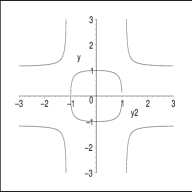
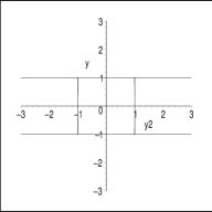
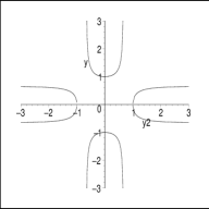
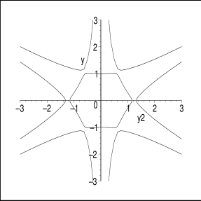
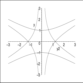
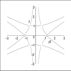
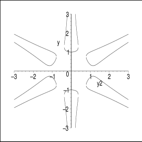
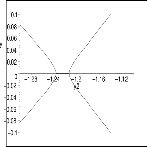
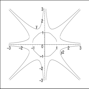
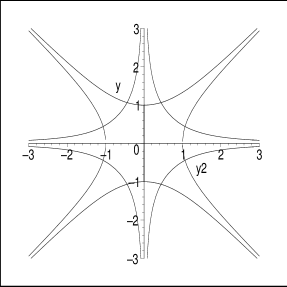
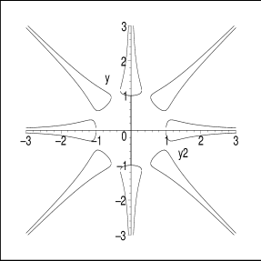
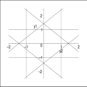
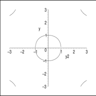
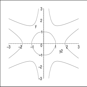
and plots of this function at different values of c𝑐c are shown in Fig.2. Distinguished point c=1𝑐1c=1 is clearly see. In terms of discriminants we have:

D(G;y2)=discrimy1(G)=4(c2y221)(y221)𝐷𝐺subscript𝑦2subscriptdiscrimsubscript𝑦1𝐺4superscript𝑐2superscriptsubscript𝑦221superscriptsubscript𝑦221\displaystyle D(G;y_{2})={\rm discrim}_{y_{1}}(G)=4(c^{2}y_{2}^{2}-1)(y_{2}^{2}-1) (4.27)

(the two branches in (4.26) merge when discriminant vanishes, either at zero or at infinity, when y2=±c1subscript𝑦2plus-or-minussuperscript𝑐1y_{2}=\pm c^{-1} and y2=±1subscript𝑦2plus-or-minus1y_{2}=\pm 1 respectively), and

discrimy2D(G;y2)=65536c2(c21)4subscriptdiscrimsubscript𝑦2𝐷𝐺subscript𝑦265536superscript𝑐2superscriptsuperscript𝑐214\displaystyle{\rm discrim}_{y_{2}}D(G;y_{2})=65536c^{2}(c^{2}-1)^{4} (4.28)

(double discriminant vanishes when branches intersect: at c=±1𝑐plus-or-minus1c=\pm 1 they do so at four points, thus zero is of the fourth power – the vertices of our square,– while at c=0𝑐0c=0 an intersection at two points takes place at infinity).

Refer to caption
Refer to caption
Refer to caption
Refer to caption
Figure 2: The plot of the function y1(y2)subscript𝑦1subscript𝑦2y_{1}(y_{2}) in (4.26) at different values of c𝑐c= 0.5, 0.87, 1 and 1.5. It is clearly seen that the unit square is formed at exactly c=1𝑐1c=1, as predicted by (4.28.

4.4.2 n=6𝑛6n=6

This time the plots for y1(y2)subscript𝑦1subscript𝑦2y_{1}(y_{2}) obtained by solving

P2=y02+1y12y22=0subscript𝑃2superscriptsubscript𝑦021superscriptsubscript𝑦12superscriptsubscript𝑦220\displaystyle P_{2}=y_{0}^{2}+1-y_{1}^{2}-y_{2}^{2}=0 (4.29)

with

y0=c3K3=cy2(3y12y22)subscript𝑦0subscript𝑐3subscript𝐾3𝑐subscript𝑦23superscriptsubscript𝑦12superscriptsubscript𝑦22\displaystyle y_{0}=c_{3}K_{3}=cy_{2}(3y_{1}^{2}-y_{2}^{2}) (4.30)

so that c=14c3𝑐14subscript𝑐3c=\frac{1}{4}c_{3}.

Discriminant

discrimy1(G)=144c2y22(c2y26y22+1)(48c2y2436c2y22+1)2subscriptdiscrimsubscript𝑦1𝐺144superscript𝑐2superscriptsubscript𝑦22superscript𝑐2superscriptsubscript𝑦26superscriptsubscript𝑦221superscript48superscript𝑐2superscriptsubscript𝑦2436superscript𝑐2superscriptsubscript𝑦2212\displaystyle{\rm discrim}_{y_{1}}(G)=144c^{2}y_{2}^{2}(c^{2}y_{2}^{6}-y_{2}^{2}+1)(48c^{2}y_{2}^{4}-36c^{2}y_{2}^{2}+1)^{2} (4.31)

Since powers appear at the r.h.s., repeated discriminant w.r.t. y2subscript𝑦2y_{2} is vanishing and we need to look at the individual factors at the r.h.s.:

discrimy2(c2y26y22+1)=64c6(27c24)2,subscriptdiscrimsubscript𝑦2superscript𝑐2superscriptsubscript𝑦26superscriptsubscript𝑦22164superscript𝑐6superscript27superscript𝑐242\displaystyle{\rm discrim}_{y_{2}}(c^{2}y_{2}^{6}-y_{2}^{2}+1)=-64c^{6}(27c^{2}-4)^{2},
discrimy2(48c2y2436c2y22+1)=1769472c6(27c24)2,subscriptdiscrimsubscript𝑦248superscript𝑐2superscriptsubscript𝑦2436superscript𝑐2superscriptsubscript𝑦2211769472superscript𝑐6superscript27superscript𝑐242\displaystyle{\rm discrim}_{y_{2}}(48c^{2}y_{2}^{4}-36c^{2}y_{2}^{2}+1)=1769472c^{6}(27c^{2}-4)^{2},
resultanty2(c2y26y22+1,+48c2y2436c2y22+1)=c8(216c2+49)4subscriptresultantsubscript𝑦2superscript𝑐2superscriptsubscript𝑦26superscriptsubscript𝑦22148superscript𝑐2superscriptsubscript𝑦2436superscript𝑐2superscriptsubscript𝑦221superscript𝑐8superscript216superscript𝑐2494\displaystyle{\rm resultant}_{y_{2}}(c^{2}y_{2}^{6}-y_{2}^{2}+1,+48c^{2}y_{2}^{4}-36c^{2}y_{2}^{2}+1)=c^{8}(216c^{2}+49)^{4} (4.32)

The interesting critical values of c𝑐c are zeroes of 27c2427superscript𝑐2427c^{2}-4, i.e. c=±239=±0.38490𝑐plus-or-minus239plus-or-minus0.38490c=\pm\frac{2\sqrt{3}}{9}=\pm 0.38490\ldots. Figs.3-6 show exact meaning of these calculations and preceding argumentation.

Refer to caption
Refer to caption
Figure 3: The plot of y1(y2)subscript𝑦1subscript𝑦2y_{1}(y_{2}) at c=1/4𝑐14c=1/4 (left) and at c=2391100𝑐2391100c=\frac{2\sqrt{3}}{9}-\frac{1}{100} (right). In the left picture the central domain is far from being a polygon: at this value of c𝑐c it looks almost like a circle (and will get even closer to this shape for smaller |c|𝑐|c|). The right picture shows what happens in a close vicinity of the critical value of c=239𝑐239c=\frac{2\sqrt{3}}{9}. The central domain still does not possess angles, see also Fig.6, but is already close to that. Note that parameter c𝑐c here is different from c00(6)superscriptsubscript𝑐006c_{00}^{(6)} in [1]: c=14c00(6)𝑐14superscriptsubscript𝑐006c=\frac{1}{4}c_{00}^{(6)}.


Refer to caption
Figure 4: The plot of y2(y1)subscript𝑦2subscript𝑦1y_{2}(y_{1}) at the critical value of c=239𝑐239c=\frac{2\sqrt{3}}{9}. Angles are well seen at the intersections of different branches, the central domain looks similar to a hexagonal polygon. Despite angles exist, the sides are not exactly straight: (4.30) satisfies boundary conditions (and also NG equations) only approximately, this value of c𝑐c is distinguished by existence of angles.


Refer to caption
Refer to caption
Figure 5: The plot of y1(y2)subscript𝑦1subscript𝑦2y_{1}(y_{2}) at c=239+1100𝑐2391100c=\frac{2\sqrt{3}}{9}+\frac{1}{100} (left), in close vicinity of the critical value of 239239\frac{2\sqrt{3}}{9}, and at c=12𝑐12c=\frac{1}{2} (right), a little further away. Different branches are now intersecting at complex values y𝑦y-variables, and the central domain is no longer closed.


Refer to caption
Refer to caption
Figure 6: Enlarged pictures, showing the vicinity of the branches merging point at c=23921000𝑐23921000c=\frac{2\sqrt{3}}{9}-\frac{2}{1000} (left picture) and c=239+21000𝑐23921000c=\frac{2\sqrt{3}}{9}+\frac{2}{1000} (right picture) – i.e. at the very close vicinity of the critical point c=239𝑐239c=\frac{2\sqrt{3}}{9}. Clearly, no angles are present at ”microscopic” level. They appear exactly at the critical point, where the two branches intersect.

4.4.3 n=8𝑛8n=8

This time

y0=c4K4=cy1y2(y12y22),subscript𝑦0subscript𝑐4subscript𝐾4𝑐subscript𝑦1subscript𝑦2superscriptsubscript𝑦12superscriptsubscript𝑦22\displaystyle y_{0}=c_{4}K_{4}=cy_{1}y_{2}(y_{1}^{2}-y_{2}^{2}), (4.33)

so that c=12c4𝑐12subscript𝑐4c=\frac{1}{2}c_{4}, the plots for y2(y1)subscript𝑦2subscript𝑦1y_{2}(y_{1}) are shown in Fig.7 and discriminants are:

discrimy1(G)=64c6y26(y221)g2(y2,c),subscriptdiscrimsubscript𝑦1𝐺64superscript𝑐6superscriptsubscript𝑦26superscriptsubscript𝑦221superscript𝑔2subscript𝑦2𝑐\displaystyle{\rm discrim}_{y_{1}}(G)=64c^{6}y_{2}^{6}(y_{2}^{2}-1)g^{2}(y_{2},c),
g(y2,c)=427c2y22+90c2y2471c2y264c4y210+8c4y212,𝑔subscript𝑦2𝑐427superscript𝑐2superscriptsubscript𝑦2290superscript𝑐2superscriptsubscript𝑦2471superscript𝑐2superscriptsubscript𝑦264superscript𝑐4superscriptsubscript𝑦2108superscript𝑐4superscriptsubscript𝑦212\displaystyle g(y_{2},c)=4-27c^{2}y_{2}^{2}+90c^{2}y_{2}^{4}-71c^{2}y_{2}^{6}-4c^{4}y_{2}^{10}+8c^{4}y_{2}^{12},
discrimy2g=137438953472c44(16c227)4(243c2+4913)6subscriptdiscrimsubscript𝑦2𝑔137438953472superscript𝑐44superscript16superscript𝑐2274superscript243superscript𝑐249136\displaystyle{\rm discrim}_{y_{2}}g=137438953472c^{44}(16c^{2}-27)^{4}(243c^{2}+4913)^{6} (4.34)

so that the relevant zero is c=334𝑐334c=\frac{3\sqrt{3}}{4}.


Refer to caption
Refer to caption
Refer to caption
Figure 7: The analogues of Figs.3-5 for n=8𝑛8n=8 with y0=cK4=cy1y2(y12y22)subscript𝑦0𝑐subscript𝐾4𝑐subscript𝑦1subscript𝑦2superscriptsubscript𝑦12superscriptsubscript𝑦22\ y_{0}=cK_{4}=cy_{1}y_{2}(y_{1}^{2}-y_{2}^{2})\ at c=1𝑐1\ c=1, c=334𝑐334\ c=\frac{3\sqrt{3}}{4} (the critical value) and c=32𝑐32\ c=\frac{3}{2}. At critical value the branches intersect at non-trivial angles, but the sides of emerging octagon are not straight: boundary conditions (and NG equations) are matched only approximately. The sides look ”more straight” in the left picture – for c𝑐c below the critical point, where angles are less pronounced: this illustrates the thesis that different criteria lead to slightly different values of the matching parameter c𝑐c. This choice of parameter is different from c00(8)superscriptsubscript𝑐008c_{00}^{(8)} in [1]: c=12c00(8)𝑐12superscriptsubscript𝑐008c=\frac{1}{2}c_{00}^{(8)}.

4.5 Exact solutions to (4.16)

The angle-sharpening problem can actually be reversed: one can consider (4.16) as an equation for G(y1,y2)𝐺subscript𝑦1subscript𝑦2G(y_{1},y_{2}). In [1] we already showed exact solutions to this problem:

GΠ=KΠ2+(1y2)QΠ2=PΠ=ofΠsegmentsP|,subscript𝐺Πsuperscriptsubscript𝐾Π21superscript𝑦2superscriptsubscript𝑄Π2subscript𝑃ΠsubscriptproductsuperscriptofΠsegmentssubscript𝑃|\displaystyle G_{\Pi}=K_{\Pi}^{2}+(1-y^{2})Q_{\Pi}^{2}=P_{\Pi}=\prod_{\stackrel{{\scriptstyle{\rm segments}}}{{{\rm of}\ \Pi}}}P_{|}, (4.35)

are totally decomposed into a product of linear functions, associated with individual segments, see (2.8). The corresponding analogues of Figs.3-7 are just 666 or 888 straight lines which form the regular hexagon and octagon at the intersection, see Fig.8. In formulas for (4.35) this looks like:

n=4::𝑛4absent\displaystyle n=4: (y1y2)2+(1y2)=(1y1)(1+y1)(1y2)(1+y2),superscriptsubscript𝑦1subscript𝑦221superscript𝑦21subscript𝑦11subscript𝑦11subscript𝑦21subscript𝑦2\displaystyle(y_{1}y_{2})^{2}+(1-y^{2})=(1-y_{1})(1+y_{1})(1-y_{2})(1+y_{2}),
n=6::𝑛6absent\displaystyle n=6: (y2(3y12y22)4)2+(1y2)(1y24)2=superscriptsubscript𝑦23superscriptsubscript𝑦12superscriptsubscript𝑦22421superscript𝑦2superscript1superscript𝑦242absent\displaystyle\left(\frac{y_{2}(3y_{1}^{2}-y_{2}^{2})}{4}\right)^{2}+(1-y^{2})\left(1-\frac{y^{2}}{4}\right)^{2}=
=\displaystyle= (1y1)(1cy1sy2)(1+cy1sy2)(1+y1)(1+cy1+sy2)(1cy1+sy2),1subscript𝑦11𝑐subscript𝑦1𝑠subscript𝑦21𝑐subscript𝑦1𝑠subscript𝑦21subscript𝑦11𝑐subscript𝑦1𝑠subscript𝑦21𝑐subscript𝑦1𝑠subscript𝑦2\displaystyle(1-y_{1})(1-cy_{1}-sy_{2})(1+cy_{1}-sy_{2})(1+y_{1})(1+cy_{1}+sy_{2})(1-cy_{1}+sy_{2}), (4.36)
withc=12,s=32,formulae-sequencewith𝑐12𝑠32\displaystyle{\rm with}\ \ \ c=\frac{1}{2},\ \ \ s=\frac{\sqrt{3}}{2},
\displaystyle\ldots

These examples are provided by the knowledge of boundary rings, their perturbation like (2.14) should give rise to more solutions and (4.16) can serve as one more property of 𝒫Πsubscript𝒫Π{\cal P}_{\Pi}, to be added to the list in s.2.5.


Refer to caption
Refer to caption
Figure 8: The analogues of Figs.3-5 for n=6𝑛6n=6 with y0=K3(114y2)subscript𝑦0subscript𝐾3114superscript𝑦2\ y_{0}=\frac{K_{3}}{(1-\frac{1}{4}y^{2})} and of Fig.7 for n=8𝑛8n=8 with y0=K4(112y2)subscript𝑦0subscript𝐾4112superscript𝑦2\ y_{0}=\frac{K_{4}}{(1-\frac{1}{2}y^{2})} which satisfy the boundary condition exactly. Ideal hexagon and octagon with sharp angles and straight sides are clearly seen in the pictures.

5 NG solution for generic skew quadrilateral

Solutions to the σ𝜎\sigma-model and NG equations with such boundary conditions were considered in [13] and [23] respectively. Though the single-parametric rhombus family, originally introduced in [32, 4], is sufficient for direct application to string-gauge duality studies, generic solutions are definitely interesting from the point of view of Plateau problem. The difficulty is that in [23] NG solution is not represented in the resolved form, as y0(y1,y2)subscript𝑦0subscript𝑦1subscript𝑦2y_{0}(y_{1},y_{2}), it is left in a parametric representation, inherited from the σ𝜎\sigma-model solution of [13]. The situation is similar to the rhombic solution, which is transformed from the parametric representation of [32, 4, 13] to resolved expression only in s.2.6 of [1].

5.1 Solutions from [13, 23]

For n=4𝑛4n=4 coordinate system can always be rotated so, that the boundary conditions and thus a solution (the one which does not correspond to spontaneously broken Z2subscript𝑍2Z_{2}-symmetry y3y3subscript𝑦3subscript𝑦3y_{3}\rightarrow-y_{3}) have y3=0subscript𝑦30y_{3}=0. The skew quadrilateral ΠΠ\Pi is formed by four null-vectors only provided Π¯¯Π\bar{\Pi} possesses an inscribed circle, thus the conditions (1.4) can always be imposed. It is only important to remember that in this form it requires the special choice of coordinate system: y1=y2=0subscript𝑦1subscript𝑦20y_{1}=y_{2}=0 at the center of the circle, and y0=0subscript𝑦00y_{0}=0 at its tangent points with the sides of the quadrilateral (if y0subscript𝑦0y_{0} vanishes at any of these points, it automatically does so at the other three). Thus NG solution is described by a single function y0(y1,y2)subscript𝑦0subscript𝑦1subscript𝑦2y_{0}(y_{1},y_{2}).

In [13, 23] it is instead described in a very different way: r𝑟r and 𝐲=(y0;y1,y2)𝐲subscript𝑦0subscript𝑦1subscript𝑦2{\bf y}=(y_{0};y_{1},y_{2}) are expressed through the variables z=1/r𝑧1𝑟z=1/r and 𝐯=z𝐲𝐯𝑧𝐲{\bf v}=z{\bf y}, which are actually the embedding (most natural) coordinates for AdS𝐴𝑑𝑆AdS σ𝜎\sigma-model. In these variables generic solution looks simple:

z=z1(ek1u+ek1u)+z2(ek2u+ek2u),𝑧subscript𝑧1superscript𝑒subscript𝑘1𝑢superscript𝑒subscript𝑘1𝑢subscript𝑧2superscript𝑒subscript𝑘2𝑢superscript𝑒subscript𝑘2𝑢\displaystyle z=z_{1}(e^{\vec{k}_{1}\vec{u}}+e^{-\vec{k}_{1}\vec{u}})+z_{2}(e^{\vec{k}_{2}\vec{u}}+e^{-\vec{k}_{2}\vec{u}}),
𝐯=𝐯1ek1u+𝐯3ek1u+𝐯2ek2u+𝐯4ek2u𝐯subscript𝐯1superscript𝑒subscript𝑘1𝑢subscript𝐯3superscript𝑒subscript𝑘1𝑢subscript𝐯2superscript𝑒subscript𝑘2𝑢subscript𝐯4superscript𝑒subscript𝑘2𝑢\displaystyle{\bf v}={\bf v}_{1}e^{\vec{k}_{1}\vec{u}}+{\bf v}_{3}e^{-\vec{k}_{1}\vec{u}}+{\bf v}_{2}e^{\vec{k}_{2}\vec{u}}+{\bf v}_{4}e^{-\vec{k}_{2}\vec{u}} (5.1)

Remaining parameters are constrained by NG equations and boundary conditions. The latter imply that

𝐯a+1za+1𝐯aza=𝐩a,a=1,2,3,4formulae-sequencesubscript𝐯𝑎1subscript𝑧𝑎1subscript𝐯𝑎subscript𝑧𝑎subscript𝐩𝑎𝑎1234\displaystyle\frac{{\bf v}_{a+1}}{z_{a+1}}-\frac{{\bf v}_{a}}{z_{a}}={\bf p}_{a},\ \ \ \ a=1,2,3,4 (5.2)

where 𝐩asubscript𝐩𝑎{\bf p}_{a} are the four null-vectors, forming the sides of our polygon ΠΠ\Pi (i.e. external momenta of the four gluons). The former imply that

z1=z3=12s=12𝐩1𝐩2,z2=z4=12t=12𝐩2𝐩3=12𝐩1𝐩4,formulae-sequencesubscript𝑧1subscript𝑧312𝑠12subscript𝐩1subscript𝐩2subscript𝑧2subscript𝑧412𝑡12subscript𝐩2subscript𝐩312subscript𝐩1subscript𝐩4\displaystyle z_{1}=z_{3}=\frac{1}{\sqrt{2s}}=\frac{1}{2\sqrt{{\bf p}_{1}{\bf p}_{2}}},\ \ \ z_{2}=z_{4}=\frac{1}{\sqrt{2t}}=\frac{1}{2\sqrt{{\bf p}_{2}{\bf p}_{3}}}=\frac{1}{2\sqrt{{\bf p}_{1}{\bf p}_{4}}},
s=(𝐩1+𝐩2)2=2𝐩1𝐩2,t=(𝐩2+𝐩3)2=2𝐩2𝐩3formulae-sequence𝑠superscriptsubscript𝐩1subscript𝐩222subscript𝐩1subscript𝐩2𝑡superscriptsubscript𝐩2subscript𝐩322subscript𝐩2subscript𝐩3\displaystyle s=({\bf p}_{1}+{\bf p}_{2})^{2}=2{\bf p}_{1}{\bf p}_{2},\ \ \ t=({\bf p}_{2}+{\bf p}_{3})^{2}=2{\bf p}_{2}{\bf p}_{3} (5.3)

Our usual variables are:

r=1z,𝐲=𝐯zformulae-sequence𝑟1𝑧𝐲𝐯𝑧\displaystyle r=\frac{1}{z},\ \ \ {\bf y}=\frac{{\bf v}}{z} (5.4)

5.2 From 𝐲(u)𝐲𝑢{\bf y}(\vec{u}) to y0(y1,y2)subscript𝑦0subscript𝑦1subscript𝑦2y_{0}(y_{1},y_{2})

Our goal is to express y0subscript𝑦0y_{0} through y1subscript𝑦1y_{1} and y2subscript𝑦2y_{2}, i.e. to eliminate two variables u𝑢\vec{u} from the three-component vector equation (5.1) for 𝐲=z1𝐯𝐲superscript𝑧1𝐯{\bf y}=z^{-1}{\bf v}. Our strategy is to reformulate the problem in terms of polynomials and then solve it with the standard methods of non-linear algebra [36]. In result we obtain y0subscript𝑦0y_{0} as a solution to quadratic equation, which will be afterwards compared with the results from boundary ring considerations.

Our equations become polynomial in terms of Uek1u𝑈superscript𝑒subscript𝑘1𝑢U\equiv e^{\vec{k}_{1}\vec{u}} and Wek2u𝑊superscript𝑒subscript𝑘2𝑢W\equiv e^{\vec{k}_{2}\vec{u}}:

z1(𝐲𝐲A)U+z2(𝐲𝐲B)W+z1(𝐲𝐲C)U1+z2(𝐲𝐲D)W1=𝟎subscript𝑧1𝐲subscript𝐲𝐴𝑈subscript𝑧2𝐲subscript𝐲𝐵𝑊subscript𝑧1𝐲subscript𝐲𝐶superscript𝑈1subscript𝑧2𝐲subscript𝐲𝐷superscript𝑊10\displaystyle z_{1}({\bf y}-{\bf y}_{A})U+z_{2}({\bf y}-{\bf y}_{B})W+z_{1}({\bf y}-{\bf y}_{C})U^{-1}+z_{2}({\bf y}-{\bf y}_{D})W^{-1}={\bf 0} (5.5)

where the four vertices are now denoted by A,B,C,D𝐴𝐵𝐶𝐷A,B,C,D, see Fig.9, and 𝐲a=𝐯azasubscript𝐲𝑎subscript𝐯𝑎subscript𝑧𝑎{\bf y}_{a}=\frac{{\bf v}_{a}}{z_{a}}, with a=A,B,C,D𝑎𝐴𝐵𝐶𝐷a=A,B,C,D, zA=zC=z1subscript𝑧𝐴subscript𝑧𝐶subscript𝑧1z_{A}=z_{C}=z_{1}, zB=zD=z2subscript𝑧𝐵subscript𝑧𝐷subscript𝑧2z_{B}=z_{D}=z_{2}, are the values of 𝐲𝐲{\bf y} at these vertices. Of course, resolvability of the system (5.5) in four variables U,U1,W,W1𝑈superscript𝑈1𝑊superscript𝑊1U,U^{-1},W,W^{-1} requires that the 4×4444\times 4 determinant vanishes – and this is guaranteed by the possibility to choose all 333-components of 𝐲𝐲{\bf y} and 𝐲asubscript𝐲𝑎{\bf y}_{a} vanishing, so that vectors in (5.5) have only three components, 0,1,20120,1,2. However, since of the four variables U,U1,W,W1𝑈superscript𝑈1𝑊superscript𝑊1U,U^{-1},W,W^{-1} only two are algebraically independent the vanishing of 4×4444\times 4 determinant is not the only resolvability condition. The more restrictive discriminantal constraint can be derived as follows.

2 = B1 = A3 = C4 = B𝐩1subscript𝐩1{\bf p}_{1}𝐩3subscript𝐩3{\bf p}_{3}𝐩2subscript𝐩2{\bf p}_{2}𝐩4subscript𝐩4{\bf p}_{4}+--+
Figure 9: Convention for labeling sides and vertices of the quadrilateral, a square is used as an example. Pluses and minuses stand for y0subscript𝑦0y_{0} increasing (+) or decreasing (-) along the vector.

Take any pair of the three equations in (5.5) and eliminate W1superscript𝑊1W^{-1} or W𝑊W:

z1(𝐊ADU+𝐊CDU1)+z2𝐊BDW=𝟎,subscript𝑧1subscript𝐊𝐴𝐷𝑈subscript𝐊𝐶𝐷superscript𝑈1subscript𝑧2subscript𝐊𝐵𝐷𝑊0\displaystyle z_{1}\Big{(}{\bf K}_{AD}U+{\bf K}_{CD}U^{-1}\Big{)}+z_{2}{\bf K}_{BD}W={\bf 0},
z1(𝐊ABU𝐊BCU1)z2𝐊BDW1=𝟎subscript𝑧1subscript𝐊𝐴𝐵𝑈subscript𝐊𝐵𝐶superscript𝑈1subscript𝑧2subscript𝐊𝐵𝐷superscript𝑊10\displaystyle z_{1}\Big{(}{\bf K}_{AB}U-{\bf K}_{BC}U^{-1}\Big{)}-z_{2}{\bf K}_{BD}W^{-1}={\bf 0} (5.6)

Here Kabλ=ϵλμνKabμνsuperscriptsubscript𝐾𝑎𝑏𝜆superscriptitalic-ϵ𝜆𝜇𝜈superscriptsubscript𝐾𝑎𝑏𝜇𝜈K_{ab}^{\lambda}=\epsilon^{\lambda\mu\nu}K_{ab}^{\mu\nu} with

Kabμν=(yμyaμ)(yνybν)(yμybμ)(yνyaν)=yμ(yaνybν)+yν(ybμyaμ)+(yaμybνybμyaν)subscriptsuperscript𝐾𝜇𝜈𝑎𝑏superscript𝑦𝜇superscriptsubscript𝑦𝑎𝜇superscript𝑦𝜈superscriptsubscript𝑦𝑏𝜈superscript𝑦𝜇superscriptsubscript𝑦𝑏𝜇superscript𝑦𝜈superscriptsubscript𝑦𝑎𝜈superscript𝑦𝜇superscriptsubscript𝑦𝑎𝜈superscriptsubscript𝑦𝑏𝜈superscript𝑦𝜈superscriptsubscript𝑦𝑏𝜇superscriptsubscript𝑦𝑎𝜇superscriptsubscript𝑦𝑎𝜇superscriptsubscript𝑦𝑏𝜈superscriptsubscript𝑦𝑏𝜇superscriptsubscript𝑦𝑎𝜈\displaystyle K^{\mu\nu}_{ab}=(y^{\mu}-y_{a}^{\mu})(y^{\nu}-y_{b}^{\nu})-(y^{\mu}-y_{b}^{\mu})(y^{\nu}-y_{a}^{\nu})=y^{\mu}(y_{a}^{\nu}-y_{b}^{\nu})+y^{\nu}(y_{b}^{\mu}-y_{a}^{\mu})+(y_{a}^{\mu}y_{b}^{\nu}-y_{b}^{\mu}y_{a}^{\nu}) (5.7)

and λ,μ,ν=0,1,2formulae-sequence𝜆𝜇𝜈012\lambda,\mu,\nu=0,1,2 is linear in y𝑦y-variables and antisymmetric in ab𝑎𝑏ab.

Picking any component of the first and any component of the second equation in (5.6) we can use WW1=1𝑊superscript𝑊11WW^{-1}=1 to obtain nine equations:

z22𝐊BD𝐊BD=z12(𝐊ADU+𝐊CDU1)(𝐊BCU𝐊ABU1)tensor-productsuperscriptsubscript𝑧22subscript𝐊𝐵𝐷subscript𝐊𝐵𝐷tensor-productsuperscriptsubscript𝑧12subscript𝐊𝐴𝐷𝑈subscript𝐊𝐶𝐷superscript𝑈1subscript𝐊𝐵𝐶𝑈subscript𝐊𝐴𝐵superscript𝑈1\displaystyle z_{2}^{2}{\bf K}_{BD}\otimes{\bf K}_{BD}=z_{1}^{2}\Big{(}{\bf K}_{AD}U+{\bf K}_{CD}U^{-1}\Big{)}\otimes\Big{(}{\bf K}_{BC}U-{\bf K}_{AB}U^{-1}\Big{)} (5.8)

or

z12𝐊AD𝐊ABU4+(z12𝐊CD𝐊ABz12𝐊AD𝐊BC+z22𝐊BD𝐊BD)U2z12𝐊CD𝐊BC=𝟎×𝟎tensor-productsuperscriptsubscript𝑧12subscript𝐊𝐴𝐷subscript𝐊𝐴𝐵superscript𝑈4tensor-productsuperscriptsubscript𝑧12subscript𝐊𝐶𝐷subscript𝐊𝐴𝐵tensor-productsuperscriptsubscript𝑧12subscript𝐊𝐴𝐷subscript𝐊𝐵𝐶tensor-productsuperscriptsubscript𝑧22subscript𝐊𝐵𝐷subscript𝐊𝐵𝐷superscript𝑈2tensor-productsuperscriptsubscript𝑧12subscript𝐊𝐶𝐷subscript𝐊𝐵𝐶00\displaystyle z_{1}^{2}{\bf K}_{AD}\otimes{\bf K}_{AB}U^{4}+\Big{(}z_{1}^{2}{\bf K}_{CD}\otimes{\bf K}_{AB}-z_{1}^{2}{\bf K}_{AD}\otimes{\bf K}_{BC}+z_{2}^{2}{\bf K}_{BD}\otimes{\bf K}_{BD}\Big{)}U^{2}-z_{1}^{2}{\bf K}_{CD}\otimes{\bf K}_{BC}={\bf 0}\times{\bf 0} (5.9)

Consistency of any pair of these equations is a non-trivial condition on 𝐊𝐊{\bf K} (all 363636 pairs are giving rise to equivalent y0(y1,y2)subscript𝑦0subscript𝑦1subscript𝑦2y_{0}(y_{1},y_{2})!). According to [36],

β,γ=±2Tαβγxβxγ=0superscriptsubscript𝛽𝛾plus-or-minus2subscript𝑇𝛼𝛽𝛾subscript𝑥𝛽subscript𝑥𝛾0\displaystyle\sum_{\beta,\gamma=\pm}^{2}T_{\alpha\beta\gamma}x_{\beta}x_{\gamma}=0 (5.10)

is resolvable system of two equations (with α=1,2𝛼12\alpha=1,2) for two variables x+,xsubscript𝑥subscript𝑥x_{+},x_{-} iff its resultant R2|2subscript𝑅conditional22R_{2|2} – which in this case coincides with the Cayley discriminant or ”hyperdeterminant” [38], see Fig.10,– vanishes:

D2|3(T)=εαα′′εαα′′′ϵββϵγγϵβ′′β′′′ϵγ′′γ′′′TαβγTαβγTα′′β′′γ′′Tα′′′β′′′γ′′′=subscript𝐷conditional23𝑇superscript𝜀𝛼superscript𝛼′′superscript𝜀superscript𝛼superscript𝛼′′′superscriptitalic-ϵ𝛽superscript𝛽superscriptitalic-ϵ𝛾superscript𝛾superscriptitalic-ϵsuperscript𝛽′′superscript𝛽′′′superscriptitalic-ϵsuperscript𝛾′′superscript𝛾′′′subscript𝑇𝛼𝛽𝛾subscript𝑇superscript𝛼superscript𝛽superscript𝛾subscript𝑇superscript𝛼′′superscript𝛽′′superscript𝛾′′subscript𝑇superscript𝛼′′′superscript𝛽′′′superscript𝛾′′′absent\displaystyle D_{2|3}(T)=\varepsilon^{\alpha\alpha^{\prime\prime}}\varepsilon^{\alpha^{\prime}\alpha^{\prime\prime\prime}}\epsilon^{\beta\beta^{\prime}}\epsilon^{\gamma\gamma^{\prime}}\epsilon^{\beta^{\prime\prime}\beta^{\prime\prime\prime}}\epsilon^{\gamma^{\prime\prime}\gamma^{\prime\prime\prime}}T_{\alpha\beta\gamma}T_{\alpha^{\prime}\beta^{\prime}\gamma^{\prime}}T_{\alpha^{\prime\prime}\beta^{\prime\prime}\gamma^{\prime\prime}}T_{\alpha^{\prime\prime\prime}\beta^{\prime\prime\prime}\gamma^{\prime\prime\prime}}=
=(T1++T2T1T2++)2+4(T1+T2++T1++T+)(T1+T2T1T2+)=0absentsuperscriptsubscript𝑇limit-from1subscript𝑇limit-from2subscript𝑇limit-from1subscript𝑇limit-from224subscript𝑇limit-from1subscript𝑇limit-from2subscript𝑇limit-from1subscript𝑇absentsubscript𝑇limit-from1subscript𝑇limit-from2subscript𝑇limit-from1subscript𝑇limit-from20\displaystyle=(T_{1++}T_{2--}-T_{1--}T_{2++})^{2}+4(T_{1+-}T_{2++}-T_{1++}T_{+-})(T_{1+-}T_{2--}-T_{1--}T_{2+-})=0 (5.11)

Of course, this is nothing but the condition that two quadratic equations have a common root and can be derived by elementary means, say, from explicit knowledge of the formula for the roots. In our case x+=U2subscript𝑥superscript𝑈2x_{+}=U^{2}, x=1subscript𝑥1x_{-}=1, and tensor Tαβγsubscript𝑇𝛼𝛽𝛾T_{\alpha\beta\gamma} is made out of 𝐊𝐊tensor-product𝐊𝐊{\bf K}\otimes{\bf K}. Discriminant D2|3subscript𝐷conditional23D_{2|3} is bilinear in both components of T1..T_{1..} and T2..T_{2..}, while Kλsuperscript𝐾𝜆{K^{\lambda}} is linear in the complementary y𝑦y-variables (i.e. in yμsuperscript𝑦𝜇y^{\mu} with μλ𝜇𝜆\mu\neq\lambda. Thus discriminantal condition can be made quadratic in y0subscript𝑦0y_{0} if we choose as a pair of equations from (5.9) either K0K1superscript𝐾0superscript𝐾1K^{0}K^{1} and K0K0superscript𝐾0superscript𝐾0K^{0}K^{0} or K0K2superscript𝐾0superscript𝐾2K^{0}K^{2} and K0K0superscript𝐾0superscript𝐾0K^{0}K^{0}. Indeed, K0superscript𝐾0K^{0} is independent of y0subscript𝑦0y_{0}, while K1superscript𝐾1K^{1} and K2superscript𝐾2K^{2} are linear in y0subscript𝑦0y_{0}, thus the corresponding discriminants will be quadratic. Instead, both expressions are a priori asymmetric in y1subscript𝑦1y_{1} and y2subscript𝑦2y_{2}, one can also consider a linear combination K0(μK1+νK2)superscript𝐾0𝜇superscript𝐾1𝜈superscript𝐾2K^{0}(\mu K^{1}+\nu K^{2}) to put this asymmetry under control.


Figure 10: Feynman diagram for the Cayley hyperdeterminant (5.11). Tensor Tαβγsubscript𝑇𝛼𝛽𝛾T_{\alpha\beta\gamma} stands at the valence-three vertices, while propagators are ϵitalic-ϵ\epsilon-symbols. See [36] for more explanations.

Example: In the case of the square we have, see Fig.9:

𝐩1=(2;0,2),𝐩2=(2;2,0),𝐩3=(2;0,2),𝐩4=(2;2,0),z1=z2=14formulae-sequencesubscript𝐩1202formulae-sequencesubscript𝐩2220formulae-sequencesubscript𝐩3202formulae-sequencesubscript𝐩4220subscript𝑧1subscript𝑧214\displaystyle{\bf p}_{1}=(2;0,2),\ \ \ {\bf p}_{2}=(-2;-2,0),\ \ \ {\bf p}_{3}=(2;0,-2),\ \ \ {\bf p}_{4}=(-2;2,0),\ \ \ \ \ \ z_{1}=z_{2}=\frac{1}{4} (5.12)

and

𝐲A=(1;1,1),𝐲B=(1;1,1),𝐲C=(1;1,1),𝐲D=(1;1,1),formulae-sequencesubscript𝐲𝐴111formulae-sequencesubscript𝐲𝐵111formulae-sequencesubscript𝐲𝐶111subscript𝐲𝐷111\displaystyle{\bf y}_{A}=(-1;1,-1),\ \ \ {\bf y}_{B}=(1;1,1),\ \ \ {\bf y}_{C}=(-1;-1,1),\ \ \ {\bf y}_{D}=(1;-1,-1),\ \ \ (5.13)

so that

y0=U+WU1+W1U+W+U1+W1,subscript𝑦0𝑈𝑊superscript𝑈1superscript𝑊1𝑈𝑊superscript𝑈1superscript𝑊1\displaystyle y_{0}=\frac{-U+W-U^{-1}+W^{-1}}{U+W+U^{-1}+W^{-1}},
y1=U+WU1W1U+W+U1+W1,subscript𝑦1𝑈𝑊superscript𝑈1superscript𝑊1𝑈𝑊superscript𝑈1superscript𝑊1\displaystyle y_{1}=\frac{U+W-U^{-1}-W^{-1}}{U+W+U^{-1}+W^{-1}},
y2=U+W+U1W1U+W+U1+W1subscript𝑦2𝑈𝑊superscript𝑈1superscript𝑊1𝑈𝑊superscript𝑈1superscript𝑊1\displaystyle y_{2}=\frac{-U+W+U^{-1}-W^{-1}}{U+W+U^{-1}+W^{-1}} (5.14)

These equations are simple enough to be solved directly:

U=(1+y1)(1y2)(1y1)(1+y2),W=(1+y1)(1+y2)(1y1)(1y2)formulae-sequence𝑈1subscript𝑦11subscript𝑦21subscript𝑦11subscript𝑦2𝑊1subscript𝑦11subscript𝑦21subscript𝑦11subscript𝑦2\displaystyle U=\sqrt{\frac{(1+y_{1})(1-y_{2})}{(1-y_{1})(1+y_{2})}},\ \ \ \ W=\sqrt{\frac{(1+y_{1})(1+y_{2})}{(1-y_{1})(1-y_{2})}} (5.15)

and in this case y0(y1,y2)subscript𝑦0subscript𝑦1subscript𝑦2y_{0}(y_{1},y_{2}) is a solution to the linear equation:

y0=y1y2subscript𝑦0subscript𝑦1subscript𝑦2\displaystyle y_{0}=y_{1}y_{2} (5.16)

However, equation is essentially quadratic already in the case of rhombus [1].

5.3 Evaluating hyperdeterminant

In general resolving eqs.(5.5) is rather tedious, moreover (5.9) provides U𝑈U and W𝑊W as solutions to biquadratic equations, which are of limited practical use. However, since we need y0(y1,y2)subscript𝑦0subscript𝑦1subscript𝑦2y_{0}(y_{1},y_{2}), there is no need to find U𝑈U and W𝑊W: this function is defined by discriminantal condition and what we actually need is evaluation of hyperdeterminant. This is a straightforward calculation with a nice answer:

D2|3{𝐏+𝐐+𝐐}{𝐏𝐐+𝐐}{𝐏+𝐏𝐐+}{𝐏+𝐏𝐐}similar-tosubscript𝐷conditional23subscript𝐏subscript𝐐subscript𝐐subscript𝐏subscript𝐐subscript𝐐subscript𝐏subscript𝐏subscript𝐐subscript𝐏subscript𝐏subscript𝐐\displaystyle D_{2|3}\sim\big{\{}{\bf P}_{+}{\bf Q}_{+}{\bf Q}_{-}\big{\}}\big{\{}{\bf P}_{-}{\bf Q}_{+}{\bf Q}_{-}\big{\}}-\big{\{}{\bf P}_{+}{\bf P}_{-}{\bf Q}_{+}\big{\}}\big{\{}{\bf P}_{+}{\bf P}_{-}{\bf Q}_{-}\big{\}} (5.17)

where {𝐏𝐐𝐑}ϵλμνPλQμRν𝐏𝐐𝐑superscriptitalic-ϵ𝜆𝜇𝜈superscript𝑃𝜆superscript𝑄𝜇superscript𝑅𝜈\big{\{}{\bf P}{\bf Q}{\bf R}\big{\}}\equiv\epsilon^{\lambda\mu\nu}P^{\lambda}Q^{\mu}R^{\nu} is the mixed product of three 333-component vectors. Proportionality coefficient between the first and the second lines in (5.17) is 11-1 for Minkovski signature. Vectors 𝐏±subscript𝐏plus-or-minus{\bf P}_{\pm} and 𝐐±subscript𝐐plus-or-minus{\bf Q}_{\pm} are still another version of parametrization of (5.5):

U𝐏++U1𝐏+W𝐐++W1𝐐=0𝑈subscript𝐏superscript𝑈1subscript𝐏𝑊subscript𝐐superscript𝑊1subscript𝐐0\displaystyle U{\bf P}_{+}\ +U^{-1}{\bf P}_{-}\ +W{\bf Q}_{+}\ +W^{-1}{\bf Q}_{-}=0 (5.18)

i.e.

𝐏+=z1(𝐲𝐲A),𝐏=z1(𝐲𝐲C),𝐐+=z2(𝐲𝐲B),𝐐=z2(𝐲𝐲D)formulae-sequencesubscript𝐏subscript𝑧1𝐲subscript𝐲𝐴formulae-sequencesubscript𝐏subscript𝑧1𝐲subscript𝐲𝐶formulae-sequencesubscript𝐐subscript𝑧2𝐲subscript𝐲𝐵subscript𝐐subscript𝑧2𝐲subscript𝐲𝐷\displaystyle{\bf P}_{+}=z_{1}({\bf y}-{\bf y}_{A}),\ \ \ \ \ {\bf P}_{-}=z_{1}({\bf y}-{\bf y}_{C}),\ \ \ \ \ {\bf Q}_{+}=z_{2}({\bf y}-{\bf y}_{B}),\ \ \ \ \ {\bf Q}_{-}=z_{2}({\bf y}-{\bf y}_{D}) (5.19)

Note that D2|3subscript𝐷conditional23D_{2|3} itself is of the 161616-th power in components of 𝐏𝐏{\bf P} and 𝐐𝐐{\bf Q}, moreover it depends on particular choice of a pair of equations out of nine in (5.9). However, all these 363636 versions of D2|3subscript𝐷conditional23D_{2|3} contain one and the same factor (5.17), which is the quadratic equation for y0subscript𝑦0y_{0} that we are looking for. Quadraticity is obvious in the first line of (5.17) and is obscure in representation through scalar products, which is still also useful in applications.

5.4 Examples

Eq.(5.17) provides y0(y1,y2)subscript𝑦0subscript𝑦1subscript𝑦2y_{0}(y_{1},y_{2}) for generic quadrilateral as a function of positions of its four vertices in 𝐲𝐲{\bf y}-space. According to (5.2) these 4×3=1243124\times 3=12 components of 𝐲a=𝐯azasubscript𝐲𝑎subscript𝐯𝑎subscript𝑧𝑎{\bf y}_{a}=\frac{{\bf v}_{a}}{z_{a}} are not free parameters (i.e. can not be chosen in arbitrary way): they are expressed through 3×21=532153\times 2-1=5 components of the three independent null-vectors, constrained by the inscribed circle condition l1+l3=l2+l4subscript𝑙1subscript𝑙3subscript𝑙2subscript𝑙4l_{1}+l_{3}=l_{2}+l_{4}. Two of these five free parameters depend on the choice of the general orientation and scale, so that finally the whole pattern of boundary conditions is labeled by 333 parameters and they can be chosen in different ways.

Mixed products with 𝐏𝐏{\bf P} and 𝐐𝐐{\bf Q} from (5.19) are actually all linear in 𝐲𝐲{\bf y}:

ABD:{𝐏+𝐐+𝐐}=z1z22(𝐲([𝐲A×𝐲B]+[𝐲B×𝐲D]+[𝐲D×𝐲A]){𝐲A𝐲B𝐲D})CBD:{𝐏𝐐+𝐐}=z1z22(𝐲([𝐲C×𝐲B]+[𝐲B×𝐲D]+[𝐲D×𝐲C])+{𝐲B𝐲C𝐲D})ACB:{𝐏+𝐏𝐐+}=z12z2(𝐲([𝐲A×𝐲C]+[𝐲C×𝐲B]+[𝐲B×𝐲A])+{𝐲A𝐲B𝐲C})ACD:{𝐏+𝐏𝐐}=z12z2(𝐲([𝐲A×𝐲C]+[𝐲D×𝐲A]+[𝐲C×𝐲D]){𝐲A𝐲C𝐲D})\displaystyle\begin{array}[]{lrcccl}ABD:&\big{\{}{\bf P}_{+}{\bf Q}_{+}{\bf Q}_{-}\big{\}}&=&z_{1}z_{2}^{2}\Big{(}{\bf y}\cdot\big{(}[{\bf y}_{A}\times{\bf y}_{B}]+[{\bf y}_{B}\times{\bf y}_{D}]+[{\bf y}_{D}\times{\bf y}_{A}]\big{)}&-&\{{\bf y}_{A}{\bf y}_{B}{\bf y}_{D}\}\Big{)}\\ CBD:&\big{\{}{\bf P}_{-}{\bf Q}_{+}{\bf Q}_{-}\big{\}}&=&z_{1}z_{2}^{2}\Big{(}{\bf y}\cdot\big{(}[{\bf y}_{C}\times{\bf y}_{B}]+[{\bf y}_{B}\times{\bf y}_{D}]+[{\bf y}_{D}\times{\bf y}_{C}]\big{)}&+&\{{\bf y}_{B}{\bf y}_{C}{\bf y}_{D}\}\Big{)}\\ ACB:&\big{\{}{\bf P}_{+}{\bf P}_{-}{\bf Q}_{+}\big{\}}&=&z_{1}^{2}z_{2}\Big{(}{\bf y}\cdot\big{(}[{\bf y}_{A}\times{\bf y}_{C}]+[{\bf y}_{C}\times{\bf y}_{B}]+[{\bf y}_{B}\times{\bf y}_{A}]\big{)}&+&\{{\bf y}_{A}{\bf y}_{B}{\bf y}_{C}\}\Big{)}\\ ACD:&\big{\{}{\bf P}_{+}{\bf P}_{-}{\bf Q}_{-}\big{\}}&=&z_{1}^{2}z_{2}\Big{(}{\bf y}\cdot\big{(}[{\bf y}_{A}\times{\bf y}_{C}]+[{\bf y}_{D}\times{\bf y}_{A}]+[{\bf y}_{C}\times{\bf y}_{D}]\big{)}&-&\{{\bf y}_{A}{\bf y}_{C}{\bf y}_{D}\}\Big{)}\end{array} (5.24)

Each line in (5.24) can also be written as a sum of four 3×3333\times 3 determinants, for example,

ABD:z1z22(||y0y1y2yA0yA1yA2yB0yB1yB2||+||y0y1y2yB0yB1yB2yD0yD1yD2||+||y0y1y2yD0yD1yD2yA0yA1yA2||||yA0yA1yA2yB0yB1yB2yD0yD1yD2||)ABD:\ \ \ z_{1}z_{2}^{2}\left(\,\left|\left|\begin{array}[]{ccc}y_{0}&y_{1}&y_{2}\\ y_{A0}&y_{A1}&y_{A2}\\ y_{B0}&y_{B1}&y_{B2}\end{array}\right|\right|+\left|\left|\begin{array}[]{ccc}y_{0}&y_{1}&y_{2}\\ y_{B0}&y_{B1}&y_{B2}\\ y_{D0}&y_{D1}&y_{D2}\end{array}\right|\right|+\left|\left|\begin{array}[]{ccc}y_{0}&y_{1}&y_{2}\\ y_{D0}&y_{D1}&y_{D2}\\ y_{A0}&y_{A1}&y_{A2}\end{array}\right|\right|-\left|\left|\begin{array}[]{ccc}y_{A0}&y_{A1}&y_{A2}\\ y_{B0}&y_{B1}&y_{B2}\\ y_{D0}&y_{D1}&y_{D2}\end{array}\right|\right|\,\right)

It remains to substitute particular values of 𝐲asubscript𝐲𝑎{\bf y}_{a} and zasubscript𝑧𝑎z_{a} in order to obtain concrete equations in concrete examples.

5.4.1 Square

From Fig.9 and (5.13),

𝐲A=(1;1,1),𝐲B=(1;1,1),𝐲C=(1;1,1),𝐲D=(1;1,1)formulae-sequencesubscript𝐲𝐴111formulae-sequencesubscript𝐲𝐵111formulae-sequencesubscript𝐲𝐶111subscript𝐲𝐷111\displaystyle{\bf y}_{A}=(-1;1,-1),\ \ \ {\bf y}_{B}=(1;1,1),\ \ \ {\bf y}_{C}=(-1;-1,1),\ \ \ {\bf y}_{D}=(1;-1,-1)\ \ \ (5.25)

Substituting these vectors for lines in determinants, we obtain for the first line in (5.24):

ABD:z1z22(||y0y1y2111111||+||y0y1y2111111||+||y0y1y2111111||||111111111||)=ABD:\ \ \ z_{1}z_{2}^{2}\left(\,\left|\left|\begin{array}[]{ccc}y_{0}&y_{1}&y_{2}\\ -1&1&-1\\ 1&1&1\end{array}\right|\right|+\left|\left|\begin{array}[]{ccc}y_{0}&y_{1}&y_{2}\\ 1&1&1\\ 1&-1&-1\end{array}\right|\right|+\left|\left|\begin{array}[]{ccc}y_{0}&y_{1}&y_{2}\\ 1&-1&-1\\ -1&1&-1\end{array}\right|\right|-\left|\left|\begin{array}[]{ccc}-1&1&-1\\ 1&1&1\\ 1&-1&-1\end{array}\right|\right|\,\right)=
=4z1z22(y0+y1y21)absent4subscript𝑧1superscriptsubscript𝑧22subscript𝑦0subscript𝑦1subscript𝑦21\displaystyle=4z_{1}z_{2}^{2}(y_{0}+y_{1}-y_{2}-1) (5.26)

Similarly for the other three lines we get:

CBD:z1z22(||y0y1y2111111||+||y0y1y2111111||+||y0y1y2111111||+||111111111||)=CBD:\ \ \ z_{1}z_{2}^{2}\left(\,\left|\left|\begin{array}[]{ccc}y_{0}&y_{1}&y_{2}\\ -1&-1&1\\ 1&1&1\end{array}\right|\right|+\left|\left|\begin{array}[]{ccc}y_{0}&y_{1}&y_{2}\\ 1&1&1\\ 1&-1&-1\end{array}\right|\right|+\left|\left|\begin{array}[]{ccc}y_{0}&y_{1}&y_{2}\\ 1&-1&-1\\ -1&-1&1\end{array}\right|\right|+\left|\left|\begin{array}[]{ccc}1&1&1\\ -1&-1&1\\ 1&-1&-1\end{array}\right|\right|\,\right)=
=4z1z22(y0+y1y2+1)absent4subscript𝑧1superscriptsubscript𝑧22subscript𝑦0subscript𝑦1subscript𝑦21\displaystyle=4z_{1}z_{2}^{2}(-y_{0}+y_{1}-y_{2}+1) (5.27)
ACB:z12z2(||y0y1y2111111||+||y0y1y2111111||+||y0y1y2111111||+||111111111||)=ACB:\ \ \ z_{1}^{2}z_{2}\left(\,\left|\left|\begin{array}[]{ccc}y_{0}&y_{1}&y_{2}\\ -1&1&-1\\ -1&-1&1\end{array}\right|\right|+\left|\left|\begin{array}[]{ccc}y_{0}&y_{1}&y_{2}\\ -1&-1&1\\ 1&1&1\end{array}\right|\right|+\left|\left|\begin{array}[]{ccc}y_{0}&y_{1}&y_{2}\\ 1&1&1\\ -1&1&-1\end{array}\right|\right|+\left|\left|\begin{array}[]{ccc}-1&1&-1\\ 1&1&1\\ -1&-1&1\end{array}\right|\right|\,\right)=
=4z12z2(y0+y1+y21)absent4superscriptsubscript𝑧12subscript𝑧2subscript𝑦0subscript𝑦1subscript𝑦21\displaystyle=4z_{1}^{2}z_{2}(-y_{0}+y_{1}+y_{2}-1) (5.28)
ACD:z12z2(||y0y1y2111111||+||y0y1y2111111||+||y0y1y2111111||||111111111||)=ACD:\ \ \ z_{1}^{2}z_{2}\left(\,\left|\left|\begin{array}[]{ccc}y_{0}&y_{1}&y_{2}\\ -1&1&-1\\ -1&-1&1\end{array}\right|\right|+\left|\left|\begin{array}[]{ccc}y_{0}&y_{1}&y_{2}\\ 1&-1&-1\\ -1&1&-1\end{array}\right|\right|+\left|\left|\begin{array}[]{ccc}y_{0}&y_{1}&y_{2}\\ -1&-1&1\\ 1&-1&-1\end{array}\right|\right|-\left|\left|\begin{array}[]{ccc}-1&1&-1\\ -1&-1&1\\ 1&-1&-1\end{array}\right|\right|\,\right)=
=4z12z2(y0+y1+y2+1)absent4superscriptsubscript𝑧12subscript𝑧2subscript𝑦0subscript𝑦1subscript𝑦21\displaystyle=4z_{1}^{2}z_{2}(y_{0}+y_{1}+y_{2}+1) (5.29)

Since in this case z1=z2=14subscript𝑧1subscript𝑧214z_{1}=z_{2}=\frac{1}{4} we finally obtain for (5.17) the familiar result (5.16):

𝒮D2|3=1162((y0+y1y21)(y0+y1y2+1)(y0+y1+y21)(y0+y1+y2+1))=similar-tosubscript𝒮subscript𝐷conditional231superscript162subscript𝑦0subscript𝑦1subscript𝑦21subscript𝑦0subscript𝑦1subscript𝑦21subscript𝑦0subscript𝑦1subscript𝑦21subscript𝑦0subscript𝑦1subscript𝑦21absent\displaystyle{\cal S}_{\Box}\sim D_{2|3}=\frac{1}{16^{2}}\Big{(}(y_{0}+y_{1}-y_{2}-1)(-y_{0}+y_{1}-y_{2}+1)-(-y_{0}+y_{1}+y_{2}-1)(y_{0}+y_{1}+y_{2}+1)\Big{)}=
=1162((y1y2)2(y01)2(y1+y2)2+(y0+1)2)=164(y0y1y2)=0absent1superscript162superscriptsubscript𝑦1subscript𝑦22superscriptsubscript𝑦012superscriptsubscript𝑦1subscript𝑦22superscriptsubscript𝑦012164subscript𝑦0subscript𝑦1subscript𝑦20\displaystyle=\frac{1}{16^{2}}\Big{(}(y_{1}-y_{2})^{2}-(y_{0}-1)^{2}-(y_{1}+y_{2})^{2}+(y_{0}+1)^{2}\Big{)}=\frac{1}{64}(y_{0}-y_{1}y_{2})=0 (5.30)

5.4.2 Rhombus

y1subscript𝑦1y_{1}y2subscript𝑦2y_{2}ϕitalic-ϕ\phiθBsubscript𝜃𝐵\theta_{B}θ~Asubscript~𝜃𝐴\tilde{\theta}_{A}𝐲A=(1+b1b;B1b,B1b)subscript𝐲𝐴1𝑏1𝑏𝐵1𝑏𝐵1𝑏{\bf y}_{A}=\left(-\frac{1+b}{1-b};\frac{B}{1-b},-\frac{B}{1-b}\right)𝐲B=(1b1+b;B1+b,B1+b)subscript𝐲𝐵1𝑏1𝑏𝐵1𝑏𝐵1𝑏{\bf y}_{B}=\left(\frac{1-b}{1+b};\frac{B}{1+b},\frac{B}{1+b}\right)𝐲C=(1+b1b;B1b,B1b)subscript𝐲𝐶1𝑏1𝑏𝐵1𝑏𝐵1𝑏{\bf y}_{C}=\left(-\frac{1+b}{1-b};-\frac{B}{1-b},\frac{B}{1-b}\right)𝐲D=(1b1+b;B1+b,B1+b)subscript𝐲𝐷1𝑏1𝑏𝐵1𝑏𝐵1𝑏{\bf y}_{D}=\left(\frac{1-b}{1+b};-\frac{B}{1+b},-\frac{B}{1+b}\right)
Figure 11: Rhombus in the standard parametrization, suggested in [4]. The values of y0subscript𝑦0y_{0} are also shown, y0=0subscript𝑦00y_{0}=0 at four tangent points. The angle ϕitalic-ϕ\phi defines the direction of a normal to the rhombus side. Directions to the vertices are θA=π4subscript𝜃𝐴𝜋4\theta_{A}=-\frac{\pi}{4} (so that θ~A=2πθA=π4subscript~𝜃𝐴2𝜋subscript𝜃𝐴𝜋4\tilde{\theta}_{A}=2\pi-\theta_{A}=\frac{\pi}{4}), θB=π4subscript𝜃𝐵𝜋4\theta_{B}=\frac{\pi}{4}, θC=3π4subscript𝜃𝐶3𝜋4\theta_{C}=\frac{3\pi}{4}, θD=5π4subscript𝜃𝐷5𝜋4\theta_{D}=\frac{5\pi}{4}. Parameter B=1+b2𝐵1superscript𝑏2B=\sqrt{1+b^{2}}. External momenta 𝐩a=𝐲a+1𝐲asubscript𝐩𝑎subscript𝐲𝑎1subscript𝐲𝑎{\bf p}_{a}={\bf y}_{a+1}-{\bf y}_{a} are vectors along the sides, i.e. are given by differences between the values that 𝐲𝐲{\bf y} takes at vertices. Parameters zasubscript𝑧𝑎z_{a} are made from scalar products of these vectors and therefore are derived from the data in the picture.

According to the table in s.2.6.3 of [1], see also Fig.11,

𝐲A=(b,B,B),𝐲B=(B+;B+,b+),𝐲C=(b;B,B),𝐲D=(b+;B+,B+),formulae-sequencesubscript𝐲𝐴subscript𝑏subscript𝐵subscript𝐵formulae-sequencesubscript𝐲𝐵subscript𝐵subscript𝐵subscript𝑏formulae-sequencesubscript𝐲𝐶subscript𝑏subscript𝐵subscript𝐵subscript𝐲𝐷subscript𝑏subscript𝐵subscript𝐵\displaystyle{\bf y}_{A}=(-b_{-},-B_{-},B_{-}),\ \ \ {\bf y}_{B}=(B_{+};B_{+},b_{+}),\ \ \ {\bf y}_{C}=(-b_{-};B_{-},-B_{-}),\ \ \ {\bf y}_{D}=(b_{+};-B_{+},-B_{+}),\ \ \ (5.31)

where

b=1+b1b,b+=1b1+b,B=B1b,B+=B1+b,B=1+b2formulae-sequencesubscript𝑏1𝑏1𝑏formulae-sequencesubscript𝑏1𝑏1𝑏formulae-sequencesubscript𝐵𝐵1𝑏formulae-sequencesubscript𝐵𝐵1𝑏𝐵1superscript𝑏2\displaystyle b_{-}=\frac{1+b}{1-b},\ \ \ b_{+}=\frac{1-b}{1+b},\ \ \ B_{-}=\frac{B}{1-b},\ \ \ B_{+}=\frac{B}{1+b},\ \ \ B=\sqrt{1+b^{2}} (5.32)

The four lines in (5.24) are now

z1z22(y0y1y2bBBb+B+B++y0y1y2b+B+B+b+B+B++y0y1y2b+B+B+bBBbBBb+B+B+b+B+B+)=subscript𝑧1superscriptsubscript𝑧22normsubscript𝑦0subscript𝑦1subscript𝑦2subscript𝑏subscript𝐵subscript𝐵subscript𝑏subscript𝐵subscript𝐵normsubscript𝑦0subscript𝑦1subscript𝑦2subscript𝑏subscript𝐵subscript𝐵subscript𝑏subscript𝐵subscript𝐵normsubscript𝑦0subscript𝑦1subscript𝑦2subscript𝑏subscript𝐵subscript𝐵subscript𝑏subscript𝐵subscript𝐵normsubscript𝑏subscript𝐵subscript𝐵subscript𝑏subscript𝐵subscript𝐵subscript𝑏subscript𝐵subscript𝐵absentz_{1}z_{2}^{2}\left(\,\left|\left|\begin{array}[]{ccc}y_{0}&y_{1}&y_{2}\\ -b_{-}&B_{-}&-B_{-}\\ b_{+}&B_{+}&B_{+}\end{array}\right|\right|+\left|\left|\begin{array}[]{ccc}y_{0}&y_{1}&y_{2}\\ b_{+}&B_{+}&B_{+}\\ b_{+}&-B_{+}&-B_{+}\end{array}\right|\right|+\left|\left|\begin{array}[]{ccc}y_{0}&y_{1}&y_{2}\\ b_{+}&-B_{+}&-B_{+}\\ -b_{-}&B_{-}&-B_{-}\end{array}\right|\right|-\left|\left|\begin{array}[]{ccc}-b_{-}&B_{-}&-B_{-}\\ b_{+}&B_{+}&B_{+}\\ b_{+}&-B_{+}&-B_{+}\end{array}\right|\right|\,\right)=
=4z1z22B+(B(y0b+)+12(b++b)(y1y2))absent4subscript𝑧1superscriptsubscript𝑧22subscript𝐵subscript𝐵subscript𝑦0subscript𝑏12subscript𝑏subscript𝑏subscript𝑦1subscript𝑦2\displaystyle=4z_{1}z_{2}^{2}B_{+}\left(B_{-}(y_{0}-b_{+})+\frac{1}{2}(b_{+}+b_{-})(y_{1}-y_{2})\right) (5.33)
z1z22(y0y1y2bBBb+B+B++y0y1y2b+B+B+b+B+B++y0y1y2b+B+B+bBB+b+B+B+bBBb+B+B+)=subscript𝑧1superscriptsubscript𝑧22normsubscript𝑦0subscript𝑦1subscript𝑦2subscript𝑏subscript𝐵subscript𝐵subscript𝑏subscript𝐵subscript𝐵normsubscript𝑦0subscript𝑦1subscript𝑦2subscript𝑏subscript𝐵subscript𝐵subscript𝑏subscript𝐵subscript𝐵normsubscript𝑦0subscript𝑦1subscript𝑦2subscript𝑏subscript𝐵subscript𝐵subscript𝑏subscript𝐵subscript𝐵normsubscript𝑏subscript𝐵subscript𝐵subscript𝑏subscript𝐵subscript𝐵subscript𝑏subscript𝐵subscript𝐵absentz_{1}z_{2}^{2}\left(\,\left|\left|\begin{array}[]{ccc}y_{0}&y_{1}&y_{2}\\ -b_{-}&-B_{-}&B_{-}\\ b_{+}&B_{+}&B_{+}\end{array}\right|\right|+\left|\left|\begin{array}[]{ccc}y_{0}&y_{1}&y_{2}\\ b_{+}&B_{+}&B_{+}\\ b_{+}&-B_{+}&-B_{+}\end{array}\right|\right|+\left|\left|\begin{array}[]{ccc}y_{0}&y_{1}&y_{2}\\ b_{+}&-B_{+}&-B_{+}\\ -b_{-}&-B_{-}&B_{-}\end{array}\right|\right|+\left|\left|\begin{array}[]{ccc}b_{+}&B_{+}&B_{+}\\ -b_{-}&-B_{-}&B_{-}\\ b_{+}&-B_{+}&-B_{+}\end{array}\right|\right|\,\right)=
=4z1z22B+(B(y0b+)+12(b++b)(y1y2))absent4subscript𝑧1superscriptsubscript𝑧22subscript𝐵subscript𝐵subscript𝑦0subscript𝑏12subscript𝑏subscript𝑏subscript𝑦1subscript𝑦2\displaystyle=4z_{1}z_{2}^{2}B_{+}\left(-B_{-}(y_{0}-b_{+})+\frac{1}{2}(b_{+}+b_{-})(y_{1}-y_{2})\right) (5.34)
z12z2(y0y1y2bBBbBB+y0y1y2bBBb+B+B++y0y1y2b+B+B+bBB+bBBb+B+B+bBB)=superscriptsubscript𝑧12subscript𝑧2normsubscript𝑦0subscript𝑦1subscript𝑦2subscript𝑏subscript𝐵subscript𝐵subscript𝑏subscript𝐵subscript𝐵normsubscript𝑦0subscript𝑦1subscript𝑦2subscript𝑏subscript𝐵subscript𝐵subscript𝑏subscript𝐵subscript𝐵normsubscript𝑦0subscript𝑦1subscript𝑦2subscript𝑏subscript𝐵subscript𝐵subscript𝑏subscript𝐵subscript𝐵normsubscript𝑏subscript𝐵subscript𝐵subscript𝑏subscript𝐵subscript𝐵subscript𝑏subscript𝐵subscript𝐵absentz_{1}^{2}z_{2}\left(\,\left|\left|\begin{array}[]{ccc}y_{0}&y_{1}&y_{2}\\ -b_{-}&B_{-}&-B_{-}\\ -b_{-}&-B_{-}&B_{-}\end{array}\right|\right|+\left|\left|\begin{array}[]{ccc}y_{0}&y_{1}&y_{2}\\ -b_{-}&-B_{-}&B_{-}\\ b_{+}&B_{+}&B_{+}\end{array}\right|\right|+\left|\left|\begin{array}[]{ccc}y_{0}&y_{1}&y_{2}\\ b_{+}&B_{+}&B_{+}\\ -b_{-}&B_{-}&-B_{-}\end{array}\right|\right|+\left|\left|\begin{array}[]{ccc}-b_{-}&B_{-}&-B_{-}\\ b_{+}&B_{+}&B_{+}\\ -b_{-}&-B_{-}&B_{-}\end{array}\right|\right|\,\right)=
=4z12z2B(B+(y0+b)+12(b++b)(y1+y2))absent4superscriptsubscript𝑧12subscript𝑧2subscript𝐵subscript𝐵subscript𝑦0subscript𝑏12subscript𝑏subscript𝑏subscript𝑦1subscript𝑦2\displaystyle=4z_{1}^{2}z_{2}B_{-}\left(-B_{+}(y_{0}+b_{-})+\frac{1}{2}(b_{+}+b_{-})(y_{1}+y_{2})\right) (5.35)
z12z2(y0y1y2bBBbBB+y0y1y2b+B+B+bBB+y0y1y2bBBb+B+B+bBBbBBb+B+B+)=superscriptsubscript𝑧12subscript𝑧2normsubscript𝑦0subscript𝑦1subscript𝑦2subscript𝑏subscript𝐵subscript𝐵subscript𝑏subscript𝐵subscript𝐵normsubscript𝑦0subscript𝑦1subscript𝑦2subscript𝑏subscript𝐵subscript𝐵subscript𝑏subscript𝐵subscript𝐵normsubscript𝑦0subscript𝑦1subscript𝑦2subscript𝑏subscript𝐵subscript𝐵subscript𝑏subscript𝐵subscript𝐵normsubscript𝑏subscript𝐵subscript𝐵subscript𝑏subscript𝐵subscript𝐵subscript𝑏subscript𝐵subscript𝐵absentz_{1}^{2}z_{2}\left(\,\left|\left|\begin{array}[]{ccc}y_{0}&y_{1}&y_{2}\\ -b_{-}&B_{-}&-B_{-}\\ -b_{-}&-B_{-}&B_{-}\end{array}\right|\right|+\left|\left|\begin{array}[]{ccc}y_{0}&y_{1}&y_{2}\\ b_{+}&-B_{+}&-B_{+}\\ -b_{-}&B_{-}&-B_{-}\end{array}\right|\right|+\left|\left|\begin{array}[]{ccc}y_{0}&y_{1}&y_{2}\\ -b_{-}&-B_{-}&B_{-}\\ b_{+}&-B_{+}&-B_{+}\end{array}\right|\right|-\left|\left|\begin{array}[]{ccc}-b_{-}&B_{-}&-B_{-}\\ -b_{-}&-B_{-}&B_{-}\\ b_{+}&-B_{+}&-B_{+}\end{array}\right|\right|\,\right)=
=4z12z2B(B+(y0+b)+12(b++b)(y1+y2))absent4superscriptsubscript𝑧12subscript𝑧2subscript𝐵subscript𝐵subscript𝑦0subscript𝑏12subscript𝑏subscript𝑏subscript𝑦1subscript𝑦2\displaystyle=4z_{1}^{2}z_{2}B_{-}\left(B_{+}(y_{0}+b_{-})+\frac{1}{2}(b_{+}+b_{-})(y_{1}+y_{2})\right) (5.36)

Therefore we obtain for (5.17):

(4z1z2)2{(z2B+)2(14(b++b)2(y1y2)2B2(y0b+)2)(z1B)2(14(b++b)2(y1+y2)2B+2(y0+b)2)}=superscript4subscript𝑧1subscript𝑧22superscriptsubscript𝑧2subscript𝐵214superscriptsubscript𝑏subscript𝑏2superscriptsubscript𝑦1subscript𝑦22superscriptsubscript𝐵2superscriptsubscript𝑦0subscript𝑏2superscriptsubscript𝑧1subscript𝐵214superscriptsubscript𝑏subscript𝑏2superscriptsubscript𝑦1subscript𝑦22superscriptsubscript𝐵2superscriptsubscript𝑦0subscript𝑏2absent(4z_{1}z_{2})^{2}\left\{(z_{2}B_{+})^{2}\left(\frac{1}{4}(b_{+}+b_{-})^{2}(y_{1}-y_{2})^{2}-B_{-}^{2}(y_{0}-b_{+})^{2}\right)-(z_{1}B_{-})^{2}\left(\frac{1}{4}(b_{+}+b_{-})^{2}(y_{1}+y_{2})^{2}-B_{+}^{2}(y_{0}+b_{-})^{2}\right)\right\}=
=(4z1z2)2{(B+B)2((z12z22)y02+2(z12b+z22b+)y0+(z1b)2(z2b+)2)+=(4z_{1}z_{2})^{2}\left\{(B_{+}B_{-})^{2}\Big{(}(z_{1}^{2}-z_{2}^{2})y_{0}^{2}+2(z_{1}^{2}b_{-}+z_{2}^{2}b_{+})y_{0}+(z_{1}b_{-})^{2}-(z_{2}b_{+})^{2}\Big{)}+\right.
+14(b++b)2[((z2B+)2(z1B)2)(y12+y22)2((z2B+)2+(z1B)2)y1y2]}=(5.32)\left.+\frac{1}{4}(b_{+}+b_{-})^{2}\left[\left((z_{2}B_{+})^{2}-(z_{1}B_{-})^{2}\right)(y_{1}^{2}+y_{2}^{2})-2\left((z_{2}B_{+})^{2}+(z_{1}B_{-})^{2}\right)y_{1}y_{2}\right]\right\}\ \stackrel{{\scriptstyle(\ref{bBpars})}}{{=}}\
=(2z1z2B21b2)2{(z12z22)y02+2y0z12(1+b)2+z22(1b)21b2+(z1(1+b)1b)2(z2(1b)1+b)2+=\left(\frac{2z_{1}z_{2}B^{2}}{1-b^{2}}\right)^{2}\left\{(z_{1}^{2}-z_{2}^{2})y_{0}^{2}+2y_{0}\frac{z_{1}^{2}(1+b)^{2}+z_{2}^{2}(1-b)^{2}}{1-b^{2}}+\left(\frac{z_{1}(1+b)}{1-b}\right)^{2}-\left(\frac{z_{2}(1-b)}{1+b}\right)^{2}+\right.
+B2[(z21+b)2(z11b)2](y12+y22)2B2[(z21+b)2+(z11b)2]y1y2}=\left.+B^{2}\left[\left(\frac{z_{2}}{1+b}\right)^{2}-\left(\frac{z_{1}}{1-b}\right)^{2}\right](y_{1}^{2}+y_{2}^{2})-2B^{2}\left[\left(\frac{z_{2}}{1+b}\right)^{2}+\left(\frac{z_{1}}{1-b}\right)^{2}\right]y_{1}y_{2}\right\}=
=(8z1z2zB21b2)2((1b2)y0+b(1y02)(1+b2)y1y2)absentsuperscript8subscript𝑧1subscript𝑧2𝑧superscript𝐵21superscript𝑏221superscript𝑏2subscript𝑦0𝑏1superscriptsubscript𝑦021superscript𝑏2subscript𝑦1subscript𝑦2\displaystyle=\left(\frac{8z_{1}z_{2}zB^{2}}{1-b^{2}}\right)^{2}\Big{(}(1-b^{2})y_{0}+b(1-y_{0}^{2})-(1+b^{2})y_{1}y_{2}\Big{)} (5.37)

provided

z1=(1b)z,z2=(1+b)z,formulae-sequencesubscript𝑧11𝑏𝑧subscript𝑧21𝑏𝑧\displaystyle z_{1}=(1-b)z,\ \ \ z_{2}=(1+b)z, (5.38)

what is indeed the case for rhombus, with

z=141+b2,𝑧141superscript𝑏2\displaystyle z=\frac{1}{4\sqrt{1+b^{2}}}, (5.39)

see [4, 13].

Thus we see that exact solution to NG equations with rhombus in the role of the boundary ΠΠ\Pi is

𝒮=y1y212(1y02)sin(2ϕ)y0cos(2ϕ)=0subscript𝒮subscript𝑦1subscript𝑦2121superscriptsubscript𝑦022italic-ϕsubscript𝑦02italic-ϕ0\displaystyle{\cal S}_{\diamond}=y_{1}y_{2}-\frac{1}{2}(1-y_{0}^{2})\sin(2\phi)-y_{0}\cos(2\phi)=0 (5.40)

where

sin(2ϕ)=2b1+b2,cos(2ϕ)=1b21+b2formulae-sequence2italic-ϕ2𝑏1superscript𝑏22italic-ϕ1superscript𝑏21superscript𝑏2\displaystyle\sin(2\phi)=\frac{2b}{1+b^{2}},\ \ \ \cos(2\phi)=\frac{1-b^{2}}{1+b^{2}} (5.41)

This is in accordance with eq.(2.54) of [1].

5.4.3 Kite

Kites form a two-dimensional family of polygons Π¯¯Π{\bar{\Pi}}, which possess only one Z2subscript𝑍2Z_{2}-symmetry, y1y1subscript𝑦1subscript𝑦1y_{1}\leftrightarrow-y_{1}. We parameterize them by two angle variables α𝛼\alpha and β𝛽\beta, which are halves of the angles at two non-equivalent vertices, see Fig.12. Rhombi with symmetry, enhanced to Z2×Z2subscript𝑍2subscript𝑍2Z_{2}\times Z_{2}, y2y2subscript𝑦2subscript𝑦2y_{2}\leftrightarrow-y_{2} in addition to y1y1subscript𝑦1subscript𝑦1y_{1}\leftrightarrow-y_{1} are a one-parametric sub-family of kites with α=β𝛼𝛽\alpha=\beta. Note that for comparison with the results of s.5.4.2 one should also make a rotation of the (y1,y2)subscript𝑦1subscript𝑦2(y_{1},y_{2}) plane by π4𝜋4\frac{\pi}{4}. After this rotation the square solution (5.16) turns into

𝒮=2y0+y12y22=0subscriptsuperscript𝒮2subscript𝑦0superscriptsubscript𝑦12superscriptsubscript𝑦220\displaystyle{\cal S}^{\prime}_{\Box}=2y_{0}+y_{1}^{2}-y_{2}^{2}=0 (5.42)

and rhombic solution (5.40) – into

𝒮=2y0cos(2ϕ)+(1y02)sin(2ϕ)+y12y22=0subscriptsuperscript𝒮2subscript𝑦02italic-ϕ1superscriptsubscript𝑦022italic-ϕsuperscriptsubscript𝑦12superscriptsubscript𝑦220\displaystyle{\cal S}^{\prime}_{\diamond}=2y_{0}\cos(2\phi)+(1-y_{0}^{2})\sin(2\phi)+y_{1}^{2}-y_{2}^{2}=0 (5.43)

or

𝒮2(1b2)y0+2b(1y02)+(1+b2)(y12y22)=0similar-tosubscriptsuperscript𝒮21superscript𝑏2subscript𝑦02𝑏1superscriptsubscript𝑦021superscript𝑏2superscriptsubscript𝑦12superscriptsubscript𝑦220\displaystyle{\cal S}^{\prime}_{\diamond}\sim 2(1-b^{2})y_{0}+2b(1-y_{0}^{2})+(1+b^{2})(y_{1}^{2}-y_{2}^{2})=0 (5.44)

with ϕ=π4αitalic-ϕ𝜋4𝛼\phi=\frac{\pi}{4}-\alpha and

b=|cosαsinα|cosα+sinα𝑏𝛼𝛼𝛼𝛼\displaystyle b=\frac{|\cos\alpha-\sin\alpha|}{\cos\alpha+\sin\alpha} (5.45)
y1subscript𝑦1y_{1}y2subscript𝑦2y_{2}α𝛼\alphaα𝛼\alphaβ𝛽\betaβ𝛽\betaϕ1subscriptitalic-ϕ1\phi_{1}θ~Asubscript~𝜃𝐴\tilde{\theta}_{A}θBsubscript𝜃𝐵\theta_{B}y0=0subscript𝑦00y_{0}=0𝐲A=(1cos(α+β)sin(α+β);sinα+sinβsin(α+β),cosβcosαsin(α+β))subscript𝐲𝐴1𝛼𝛽𝛼𝛽𝛼𝛽𝛼𝛽𝛽𝛼𝛼𝛽{\bf y}_{A}=\left(-\frac{1-\cos(\alpha+\beta)}{\sin(\alpha+\beta)};\ \frac{\sin\alpha+\sin\beta}{\sin(\alpha+\beta)},\ \frac{\cos\beta-\cos\alpha}{\sin(\alpha+\beta)}\right)𝐲B=(cosαsinα; 0,1sinα)=(P;0,p)subscript𝐲𝐵𝛼𝛼 01𝛼𝑃0𝑝{\bf y}_{B}=\left(\frac{\cos\alpha}{\sin\alpha};\ 0,\ \frac{1}{\sin\alpha}\right)=\left(P;0,p\right)𝐲C=(1cos(α+β)sin(α+β);sinα+sinβsin(α+β),cosβcosαsin(α+β))subscript𝐲𝐶1𝛼𝛽𝛼𝛽𝛼𝛽𝛼𝛽𝛽𝛼𝛼𝛽{\bf y}_{C}=\left(-\frac{1-\cos(\alpha+\beta)}{\sin(\alpha+\beta)};\ -\frac{\sin\alpha+\sin\beta}{\sin(\alpha+\beta)},\ \frac{\cos\beta-\cos\alpha}{\sin(\alpha+\beta)}\right)𝐲D=(cosβsinβ; 0,1sinβ)=(Q;0,q)subscript𝐲𝐷𝛽𝛽 01𝛽𝑄0𝑞{\bf y}_{D}=\left(\frac{\cos\beta}{\sin\beta};\ 0,\ -\frac{1}{\sin\beta}\right)=\left(Q;0,q\right)=(K;k+,k)absent𝐾subscript𝑘subscript𝑘=\left(-K;k_{+},k_{-}\right)=(K;k+,k)absent𝐾subscript𝑘subscript𝑘=\left(-K;-k_{+},k_{-}\right)
Figure 12: Kite-like polygon Π¯¯Π\bar{\Pi} with only one Z2subscript𝑍2Z_{2}-symmetry, y1y1subscript𝑦1subscript𝑦1y_{1}\rightarrow-y_{1}. Kites form a two-dimensional family, parameterized by α𝛼\alpha and β𝛽\beta. Angles at four vertices are παβ𝜋𝛼𝛽\pi-\alpha-\beta at A𝐴A and C𝐶C, 2α2𝛼2\alpha at B𝐵B and 2β2𝛽2\beta at D𝐷D and directions to vertices are θA=2πθ~A=αβ2subscript𝜃𝐴2𝜋subscript~𝜃𝐴𝛼𝛽2\theta_{A}=2\pi-\tilde{\theta}_{A}=\frac{\alpha-\beta}{2}, θB=π2subscript𝜃𝐵𝜋2\theta_{B}=\frac{\pi}{2}, θC=παβ2subscript𝜃𝐶𝜋𝛼𝛽2\theta_{C}=\pi-\frac{\alpha-\beta}{2} and θD=3π2subscript𝜃𝐷3𝜋2\theta_{D}=\frac{3\pi}{2}. The four normal directions are: ϕ1=αsubscriptitalic-ϕ1𝛼\phi_{1}=\alpha, ϕ2=πϕ1=παsubscriptitalic-ϕ2𝜋subscriptitalic-ϕ1𝜋𝛼\phi_{2}=\pi-\phi_{1}=\pi-\alpha, ϕ3=π+βsubscriptitalic-ϕ3𝜋𝛽\phi_{3}=\pi+\beta and ϕ4=2πβsubscriptitalic-ϕ42𝜋𝛽\phi_{4}=2\pi-\beta. Rhombus is a particular sub-family with β=α𝛽𝛼\beta=\alpha. Note that this picture is rotated by an angle π4𝜋4\frac{\pi}{4} as compared to Fig.11.

It is a simple geometrical exercise to express the values of 𝐲𝐲{\bf y} at the kite vertices through α𝛼\alpha and β𝛽\beta. It is only important to remember that we put the radius of inscribed circle equal to one. It follows that the ordinates of the vertices B𝐵B and D𝐷D are y2B=cotαsubscript𝑦2𝐵𝛼y_{2B}=\cot\alpha and y2D=cotβsubscript𝑦2𝐷𝛽y_{2D}=\cot\beta, while the corresponding values of y0subscript𝑦0y_{0} are y0B=1sinαsubscript𝑦0𝐵1𝛼y_{0B}=\frac{1}{\sin\alpha} and y0D=1sinβsubscript𝑦0𝐷1𝛽y_{0D}=\frac{1}{\sin\beta}, because y0subscript𝑦0y_{0} vanishes at the tangent points with the unit circle. Further, the two side lengths l1=lABsubscript𝑙1subscript𝑙𝐴𝐵l_{1}=l_{AB} and l4=lDAsubscript𝑙4subscript𝑙𝐷𝐴l_{4}=l_{DA} of the kite are related through

l1cosα+l4cosβ=1sinα+1sinβ,subscript𝑙1𝛼subscript𝑙4𝛽1𝛼1𝛽\displaystyle l_{1}\cos\alpha+l_{4}\cos\beta=\frac{1}{\sin\alpha}+\frac{1}{\sin\beta},
l1sinα=l4sinβ=y1Asubscript𝑙1𝛼subscript𝑙4𝛽subscript𝑦1𝐴\displaystyle l_{1}\sin\alpha=l_{4}\sin\beta=y_{1A} (5.46)

The most convenient variables for actual calculations are t=tanα2𝑡𝛼2t=\tan\frac{\alpha}{2} and t=tanβ2superscript𝑡𝛽2t^{\prime}=\tan\frac{\beta}{2}, i.e. trigonometric functions of the quarters of the kite’s angles with values bound between 00 and 111: 0<t,t<1formulae-sequence0𝑡superscript𝑡10<t,t^{\prime}<1. Unfortunately, they are much less convenient for consideration of particular degenerations, in particular for the square t=t=tanπ8=212+1superscript𝑡𝑡𝜋82121t^{\prime}=t=\tan\frac{\pi}{8}=\sqrt{\frac{\sqrt{2}-1}{\sqrt{2}+1}}. In terms of these variables

sinα=2t1+t2,cosα=1t21+t2,sinβ=2t1+t2,cosβ=1t21+t2formulae-sequence𝛼2𝑡1superscript𝑡2formulae-sequence𝛼1superscript𝑡21superscript𝑡2formulae-sequence𝛽2superscript𝑡1superscriptsuperscript𝑡2𝛽1superscriptsuperscript𝑡21superscriptsuperscript𝑡2\displaystyle\sin\alpha=\frac{2t}{1+t^{2}},\ \ \ \cos\alpha=\frac{1-t^{2}}{1+t^{2}},\ \ \ \sin\beta=\frac{2t^{\prime}}{1+{t^{\prime}}^{2}},\ \ \ \cos\beta=\frac{1-{t^{\prime}}^{2}}{1+{t^{\prime}}^{2}} (5.47)

and

𝐲A=(1cos(α+β)sin(α+β);sinα+sinβsin(α+β),cosβcosαsin(α+β))=(K;k+,k)=(t+t1tt;1+tt1tt,tt1tt),𝐲B=(cosαsinα; 0,1sinα)=(P; 0,p)=(1t22t; 0,1+t22t),𝐲C=(1cos(α+β)sin(α+β);sinα+sinβsin(α+β),cosβcosαsin(α+β))=(K;k+,k)=(t+t1tt;1+tt1tt,tt1tt),𝐲D=(cosβsinβ; 0,1sinβ)=(Q; 0,q)=(1t22t; 0,1+t22t)subscript𝐲𝐴1𝛼𝛽𝛼𝛽𝛼𝛽𝛼𝛽𝛽𝛼𝛼𝛽𝐾subscript𝑘subscript𝑘𝑡superscript𝑡1𝑡superscript𝑡1𝑡superscript𝑡1𝑡superscript𝑡𝑡superscript𝑡1𝑡superscript𝑡missing-subexpressionmissing-subexpressionmissing-subexpressionmissing-subexpressionmissing-subexpressionsubscript𝐲𝐵𝛼𝛼 01𝛼𝑃 0𝑝1superscript𝑡22𝑡 01superscript𝑡22𝑡missing-subexpressionmissing-subexpressionmissing-subexpressionmissing-subexpressionmissing-subexpressionsubscript𝐲𝐶1𝛼𝛽𝛼𝛽𝛼𝛽𝛼𝛽𝛽𝛼𝛼𝛽𝐾subscript𝑘subscript𝑘𝑡superscript𝑡1𝑡superscript𝑡1𝑡superscript𝑡1𝑡superscript𝑡𝑡superscript𝑡1𝑡superscript𝑡missing-subexpressionmissing-subexpressionmissing-subexpressionmissing-subexpressionmissing-subexpressionsubscript𝐲𝐷𝛽𝛽 01𝛽𝑄 0𝑞1superscriptsuperscript𝑡22superscript𝑡 01superscriptsuperscript𝑡22superscript𝑡\displaystyle\begin{array}[]{ccccc}{\bf y}_{A}=\left(-\frac{1-\cos(\alpha+\beta)}{\sin(\alpha+\beta)};\ \frac{\sin\alpha+\sin\beta}{\sin(\alpha+\beta)},\ \frac{\cos\beta-\cos\alpha}{\sin(\alpha+\beta)}\right)&=&\big{(}-K;\ k_{+},\ k_{-}\big{)}&=&\left(-\frac{t+t^{\prime}}{1-tt^{\prime}};\ \frac{1+tt^{\prime}}{1-tt^{\prime}},\ \frac{t-t^{\prime}}{1-tt^{\prime}}\right),\\ &&\\ {\bf y}_{B}=\left(\frac{\cos\alpha}{\sin\alpha};\ 0,\ \frac{1}{\sin\alpha}\right)&=&\big{(}P;\ 0,\ p\big{)}&=&\left(\frac{1-t^{2}}{2t};\ 0,\ \frac{1+t^{2}}{2t}\,\right),\\ &&\\ {\bf y}_{C}=\left(-\frac{1-\cos(\alpha+\beta)}{\sin(\alpha+\beta)};\ -\frac{\sin\alpha+\sin\beta}{\sin(\alpha+\beta)},\ \frac{\cos\beta-\cos\alpha}{\sin(\alpha+\beta)}\right)&=&\big{(}-K;\ -k_{+},\ k_{-}\big{)}&=&\left(-\frac{t+t^{\prime}}{1-tt^{\prime}};\ -\frac{1+tt^{\prime}}{1-tt^{\prime}},\ \frac{t-t^{\prime}}{1-tt^{\prime}}\right),\\ &&\\ {\bf y}_{D}=\left(\frac{\cos\beta}{\sin\beta};\ 0,\ -\frac{1}{\sin\beta}\right)&=&\big{(}Q;\ 0,\ q\big{)}&=&\left(\frac{1-{t^{\prime}}^{2}}{2t^{\prime}};\ 0,\ -\frac{1+{t^{\prime}}^{2}}{2t^{\prime}}\right)\end{array} (5.55)

It follows that

z1=zA=zC=12(𝐲C𝐲B)(𝐲B𝐲A))1/2=1221tt1+tt,\displaystyle z_{1}=z_{A}=z_{C}=\frac{1}{2}\Big{(}{\bf y}_{C}-{\bf y}_{B})({\bf y}_{B}-{\bf y}_{A})\Big{)}^{-1/2}=\frac{1}{2\sqrt{2}}\frac{1-tt^{\prime}}{1+tt^{\prime}},
z2=zB=zD=12(𝐲C𝐲B)(𝐲D𝐲C))1/2=2tt2(1+tt)\displaystyle z_{2}=z_{B}=z_{D}=\frac{1}{2}\Big{(}{\bf y}_{C}-{\bf y}_{B})({\bf y}_{D}-{\bf y}_{C})\Big{)}^{-1/2}=\frac{\sqrt{2tt^{\prime}}}{2(1+tt^{\prime})} (5.56)

In terms of condensed notation, introduced in (5.55), the four lines in (5.24) are now:

ABD:z1z22(||y0y1y2Kk+kP0p||+||y0y1y2P0pQ0q||+||y0y1y2Q0qKk+k||||Kk+kP0pQ0q||)=ABD:\ \ \ z_{1}z_{2}^{2}\left(\,\left|\left|\begin{array}[]{ccc}y_{0}&y_{1}&y_{2}\\ -K&k_{+}&k_{-}\\ P&0&p\end{array}\right|\right|+\left|\left|\begin{array}[]{ccc}y_{0}&y_{1}&y_{2}\\ P&0&p\\ Q&0&q\end{array}\right|\right|+\left|\left|\begin{array}[]{ccc}y_{0}&y_{1}&y_{2}\\ Q&0&q\\ -K&k_{+}&k_{-}\end{array}\right|\right|-\left|\left|\begin{array}[]{ccc}-K&k_{+}&k_{-}\\ P&0&p\\ Q&0&q\end{array}\right|\right|\,\right)=
=z1z22{k+((pq)y0(PQ)y2+(PqQp))+(K(pq)+(PQ)k(PqQp))y1}absentsubscript𝑧1superscriptsubscript𝑧22subscript𝑘𝑝𝑞subscript𝑦0𝑃𝑄subscript𝑦2𝑃𝑞𝑄𝑝𝐾𝑝𝑞𝑃𝑄subscript𝑘𝑃𝑞𝑄𝑝subscript𝑦1\displaystyle=z_{1}z_{2}^{2}\left\{k_{+}\Big{(}(p-q)y_{0}-(P-Q)y_{2}+(Pq-Qp)\Big{)}+\Big{(}K(p-q)+(P-Q)k_{-}-(Pq-Qp)\Big{)}y_{1}\right\}
CBD:z1z22(||y0y1y2Kk+kP0p||+||y0y1y2P0pQ0q||+||y0y1y2Q0qKk+k||+||P0pKk+kQ0q||)=CBD:\ \ \ z_{1}z_{2}^{2}\left(\,\left|\left|\begin{array}[]{ccc}y_{0}&y_{1}&y_{2}\\ -K&-k_{+}&k_{-}\\ P&0&p\end{array}\right|\right|+\left|\left|\begin{array}[]{ccc}y_{0}&y_{1}&y_{2}\\ P&0&p\\ Q&0&q\end{array}\right|\right|+\left|\left|\begin{array}[]{ccc}y_{0}&y_{1}&y_{2}\\ Q&0&q\\ -K&-k_{+}&k_{-}\end{array}\right|\right|+\left|\left|\begin{array}[]{ccc}P&0&p\\ -K&-k_{+}&k_{-}\\ Q&0&q\end{array}\right|\right|\,\right)=
=z1z22{k+((pq)y0(PQ)y2+(PqQp))+(K(pq)+(PQ)k(PqQp))y1}absentsubscript𝑧1superscriptsubscript𝑧22subscript𝑘𝑝𝑞subscript𝑦0𝑃𝑄subscript𝑦2𝑃𝑞𝑄𝑝𝐾𝑝𝑞𝑃𝑄subscript𝑘𝑃𝑞𝑄𝑝subscript𝑦1\displaystyle=z_{1}z_{2}^{2}\left\{-k_{+}\Big{(}(p-q)y_{0}-(P-Q)y_{2}+(Pq-Qp)\Big{)}+\Big{(}K(p-q)+(P-Q)k_{-}-(Pq-Qp)\Big{)}y_{1}\right\}
ACB:z12z2(||y0y1y2Kk+kKk+k||+||y0y1y2Kk+kP0p||+||y0y1y2P0pKk+k||+||Kk+kP0pKk+k||)=ACB:\ \ \ z_{1}^{2}z_{2}\left(\,\left|\left|\begin{array}[]{ccc}y_{0}&y_{1}&y_{2}\\ -K&k_{+}&k_{-}\\ -K&-k_{+}&k_{-}\end{array}\right|\right|+\left|\left|\begin{array}[]{ccc}y_{0}&y_{1}&y_{2}\\ -K&-k_{+}&k_{-}\\ P&0&p\end{array}\right|\right|+\left|\left|\begin{array}[]{ccc}y_{0}&y_{1}&y_{2}\\ P&0&p\\ -K&k_{+}&k_{-}\end{array}\right|\right|+\left|\left|\begin{array}[]{ccc}-K&k_{+}&k_{-}\\ P&0&p\\ -K&-k_{+}&k_{-}\end{array}\right|\right|\,\right)=
=2k+z12z2((kp)y0+(K+P)y2(Kp+Pk))absent2subscript𝑘superscriptsubscript𝑧12subscript𝑧2subscript𝑘𝑝subscript𝑦0𝐾𝑃subscript𝑦2𝐾𝑝𝑃subscript𝑘\displaystyle=2k_{+}z_{1}^{2}z_{2}\Big{(}(k_{-}-p)y_{0}+(K+P)y_{2}-(Kp+Pk_{-})\Big{)}
ACD:z12z2(||y0y1y2Kk+kKk+k||+||y0y1y2Q0qKk+k||+||y0y1y2Kk+kQ0q||||Kk+kKk+kQ0q||)=ACD:\ \ \ z_{1}^{2}z_{2}\left(\,\left|\left|\begin{array}[]{ccc}y_{0}&y_{1}&y_{2}\\ -K&k_{+}&k_{-}\\ -K&-k_{+}&k_{-}\end{array}\right|\right|+\left|\left|\begin{array}[]{ccc}y_{0}&y_{1}&y_{2}\\ Q&0&q\\ -K&k_{+}&k_{-}\end{array}\right|\right|+\left|\left|\begin{array}[]{ccc}y_{0}&y_{1}&y_{2}\\ -K&-k_{+}&k_{-}\\ Q&0&q\end{array}\right|\right|-\left|\left|\begin{array}[]{ccc}-K&k_{+}&k_{-}\\ -K&-k_{+}&k_{-}\\ Q&0&q\end{array}\right|\right|\,\right)=
=2k+z12z2((kq)y0+(K+Q)y2(Kq+Qk))absent2subscript𝑘superscriptsubscript𝑧12subscript𝑧2subscript𝑘𝑞subscript𝑦0𝐾𝑄subscript𝑦2𝐾𝑞𝑄subscript𝑘\displaystyle=2k_{+}z_{1}^{2}z_{2}\Big{(}(k_{-}-q)y_{0}+(K+Q)y_{2}-(Kq+Qk_{-})\Big{)}

Thus (5.17) becomes:

(z1z2)2{z22(K(pq)+(PQ)k(PqQp))2y12(k+z2)2((pq)y0(PQ)y2+(PqQp))2\displaystyle(z_{1}z_{2})^{2}\left\{z_{2}^{2}\Big{(}K(p-q)+(P-Q)k_{-}-(Pq-Qp)\Big{)}^{2}y_{1}^{2}-(k_{+}z_{2})^{2}\Big{(}(p-q)y_{0}-(P-Q)y_{2}+(Pq-Qp)\Big{)}^{2}-\right.
(2k+z1)2((kp)y0+(K+P)y2(Kp+Pk))((kq)y0+(K+Q)y2(Kq+Qk))}\displaystyle\left.-(2k_{+}z_{1})^{2}\Big{(}(k_{-}-p)y_{0}+(K+P)y_{2}-(Kp+Pk_{-})\Big{)}\Big{(}(k_{-}-q)y_{0}+(K+Q)y_{2}-(Kq+Qk_{-})\Big{)}\right\}

and finally

𝒮kite=D2|3=1128(1+tt)2{((1tt)22(t2+t2))y024(tt)(t+t)y0y2+\displaystyle{\cal S}_{kite}=D_{2|3}=\frac{1}{128(1+tt^{\prime})^{2}}\Big{\{}\left((1-tt^{\prime})^{2}-2(t^{2}+{t^{\prime}}^{2})\right)y_{0}^{2}-4(t-t^{\prime})(t+t^{\prime})y_{0}y_{2}+
+(1+tt)2(y12y22)2(tt)2y22+4(1tt)((t+t)y0+(tt)y2)(16tt+(tt)2)}\displaystyle+(1+tt^{\prime})^{2}(y_{1}^{2}-y_{2}^{2})-2(t-t^{\prime})^{2}y_{2}^{2}+4(1-tt^{\prime})\Big{(}(t+t^{\prime})y_{0}+(t-t^{\prime})y_{2}\Big{)}-\big{(}1-6tt^{\prime}+(tt^{\prime})^{2}\big{)}\Big{\}} (5.57)

This expression can be also rewritten as

64𝒮kite=12(y12+y22y021)+(1t2)(1t2)(1+tt)2y02(1+t2)(1+t2)(1+tt)2y22+4tt(1+tt)264subscript𝒮𝑘𝑖𝑡𝑒12superscriptsubscript𝑦12superscriptsubscript𝑦22superscriptsubscript𝑦0211superscript𝑡21superscriptsuperscript𝑡2superscript1𝑡superscript𝑡2superscriptsubscript𝑦021superscript𝑡21superscriptsuperscript𝑡2superscript1𝑡superscript𝑡2superscriptsubscript𝑦22limit-from4𝑡superscript𝑡superscript1𝑡superscript𝑡264{\cal S}_{kite}=\frac{1}{2}(y_{1}^{2}+y_{2}^{2}-y_{0}^{2}-1)+\frac{(1-t^{2})(1-{t^{\prime}}^{2})}{(1+tt^{\prime})^{2}}y_{0}^{2}-\frac{(1+t^{2})(1+{t^{\prime}}^{2})}{(1+tt^{\prime})^{2}}y_{2}^{2}+\frac{4tt^{\prime}}{(1+tt^{\prime})^{2}}-
2(t2t2)(1+tt)2y0y2+2(1tt)(1+tt)2((t+t)y0+(tt)y2)2superscript𝑡2superscriptsuperscript𝑡2superscript1𝑡superscript𝑡2subscript𝑦0subscript𝑦221𝑡superscript𝑡superscript1𝑡superscript𝑡2𝑡superscript𝑡subscript𝑦0𝑡superscript𝑡subscript𝑦2-\frac{2(t^{2}-{t^{\prime}}^{2})}{(1+tt^{\prime})^{2}}y_{0}y_{2}+\frac{2(1-tt^{\prime})}{(1+tt^{\prime})^{2}}\Big{(}(t+t^{\prime})y_{0}+(t-t^{\prime})y_{2}\Big{)}

or, making use of (5.47) to convert back to original angular variables:

12(128𝒮kite+P2)cos(αβ)=12128subscript𝒮𝑘𝑖𝑡𝑒subscript𝑃2𝛼𝛽absent\displaystyle\frac{1}{2}\Big{(}128{\cal S}_{kite}+P_{2}\Big{)}\cos(\alpha-\beta)=
=y02cosαcosβy22+y0y2(cosαcosβ)+y0sin(α+β)+y2(sinαsinβ)+sinαsinβ=absentsuperscriptsubscript𝑦02𝛼𝛽superscriptsubscript𝑦22subscript𝑦0subscript𝑦2𝛼𝛽subscript𝑦0𝛼𝛽subscript𝑦2𝛼𝛽𝛼𝛽absent\displaystyle=y_{0}^{2}\cos\alpha\cos\beta-y_{2}^{2}+y_{0}y_{2}(\cos\alpha-\cos\beta)+y_{0}\sin(\alpha+\beta)+y_{2}(\sin\alpha-\sin\beta)+\sin\alpha\sin\beta=
=y02cosαcosβ+y0y2(cosαcosβ)+y0sin(α+β)+(sinαy2)(sinβ+y2)absentsuperscriptsubscript𝑦02𝛼𝛽subscript𝑦0subscript𝑦2𝛼𝛽subscript𝑦0𝛼𝛽𝛼subscript𝑦2𝛽subscript𝑦2\displaystyle=y_{0}^{2}\cos\alpha\cos\beta+y_{0}y_{2}(\cos\alpha-\cos\beta)+y_{0}\sin(\alpha+\beta)+(\sin\alpha-y_{2})(\sin\beta+y_{2}) (5.58)

5.4.4 A version of parametrization for generic quadrilateral case

y1subscript𝑦1y_{1}y2subscript𝑦2y_{2}αB=π2φBsubscript𝛼𝐵𝜋2subscript𝜑𝐵\alpha_{B}=\frac{\pi}{2}-\varphi_{B}αBsubscript𝛼𝐵\alpha_{B}B𝐵BαA=π2φAsubscript𝛼𝐴𝜋2subscript𝜑𝐴\alpha_{A}=\frac{\pi}{2}-\varphi_{A}A𝐴AαAsubscript𝛼𝐴\alpha_{A}θB=φBsubscript𝜃𝐵subscript𝜑𝐵\theta_{B}=\varphi_{B}φBsubscript𝜑𝐵\varphi_{B}φAsubscript𝜑𝐴\varphi_{A}θA=2πφAsubscript𝜃𝐴2𝜋subscript𝜑𝐴\theta_{A}=2\pi-\varphi_{A}φBsubscript𝜑𝐵\varphi_{B}φCsubscript𝜑𝐶\varphi_{C}φCsubscript𝜑𝐶\varphi_{C}φDsubscript𝜑𝐷\varphi_{D}φDsubscript𝜑𝐷\varphi_{D}φAsubscript𝜑𝐴\varphi_{A}ϕ2=π2αBsubscriptitalic-ϕ2𝜋2subscript𝛼𝐵\phi_{2}=\pi-2\alpha_{B}θC=2φB+φCsubscript𝜃𝐶2subscript𝜑𝐵subscript𝜑𝐶\theta_{C}=2\varphi_{B}+\varphi_{C}C𝐶Cϕ3=2φB+2φCsubscriptitalic-ϕ32subscript𝜑𝐵2subscript𝜑𝐶\phi_{3}=2\varphi_{B}+2\varphi_{C}=2π2φA2φDabsent2𝜋2subscript𝜑𝐴2subscript𝜑𝐷=2\pi-2\varphi_{A}-2\varphi_{D}ϕ1=0subscriptitalic-ϕ10\phi_{1}=0ϕ4=2π2φAsubscriptitalic-ϕ42𝜋2subscript𝜑𝐴\phi_{4}=2\pi-2\varphi_{A}𝐲A=(tanφA; 1,tanφA)subscript𝐲𝐴subscript𝜑𝐴1subscript𝜑𝐴{\bf y}_{A}=\Big{(}-\tan\varphi_{A};\ 1,\ -\tan\varphi_{A}\Big{)}𝐲B=(tanφB; 1,tanφB)subscript𝐲𝐵subscript𝜑𝐵1subscript𝜑𝐵{\bf y}_{B}=\Big{(}\tan\varphi_{B};\ 1,\ \tan\varphi_{B}\Big{)}𝐲C=(tanφC; 1lBCsin(2φB),{\bf y}_{C}=\Big{(}-\tan\varphi_{C};\ 1-l_{BC}\sin(2\varphi_{B}),tanϕB+lBCcos(2φB))\tan\phi_{B}+l_{BC}\cos(2\varphi_{B})\Big{)}𝐲D=(tanφD; 1lADsin(2φA),tanφAlADcos(2φA))subscript𝐲𝐷subscript𝜑𝐷1subscript𝑙𝐴𝐷2subscript𝜑𝐴subscript𝜑𝐴subscript𝑙𝐴𝐷2subscript𝜑𝐴{\bf y}_{D}=\Big{(}\tan\varphi_{D};\ 1-l_{AD}\sin(2\varphi_{A}),\ -\tan\varphi_{A}-l_{AD}\cos(2\varphi_{A})\Big{)}θD=2π2φAφDsubscript𝜃𝐷2𝜋2subscript𝜑𝐴subscript𝜑𝐷\theta_{D}=2\pi-2\varphi_{A}-\varphi_{D}D𝐷D
Figure 13: Generic skew quadrilateral Π¯¯Π\bar{\Pi} is parameterized by four angles: φA,B,C,Dsubscript𝜑𝐴𝐵𝐶𝐷\varphi_{A,B,C,D}, subjected to constraint 2φA+2φB+2φC+2φD=2π2subscript𝜑𝐴2subscript𝜑𝐵2subscript𝜑𝐶2subscript𝜑𝐷2𝜋2\varphi_{A}+2\varphi_{B}+2\varphi_{C}+2\varphi_{D}=2\pi. For circle of unit radius the side lengths are l1=lAB=tanφA+tanφBsubscript𝑙1subscript𝑙𝐴𝐵subscript𝜑𝐴subscript𝜑𝐵l_{1}=l_{AB}=\tan\varphi_{A}+\tan\varphi_{B} etc. Rotation freedom is fixed by requiring that the first segment AB𝐴𝐵AB is vertical: ϕ1=0subscriptitalic-ϕ10\phi_{1}=0. Then the other three normal directions are: ϕ2=ϕBC=2φBsubscriptitalic-ϕ2subscriptitalic-ϕ𝐵𝐶2subscript𝜑𝐵\phi_{2}=\phi_{BC}=2\varphi_{B} ϕ3=ϕCD=2φB+2φC=2π2φA2φDsubscriptitalic-ϕ3subscriptitalic-ϕ𝐶𝐷2subscript𝜑𝐵2subscript𝜑𝐶2𝜋2subscript𝜑𝐴2subscript𝜑𝐷\phi_{3}=\phi_{CD}=2\varphi_{B}+2\varphi_{C}=2\pi-2\varphi_{A}-2\varphi_{D}, ϕ4=ϕDA=2π2φDsubscriptitalic-ϕ4subscriptitalic-ϕ𝐷𝐴2𝜋2subscript𝜑𝐷\phi_{4}=\phi_{DA}=2\pi-2\varphi_{D} and direction towards the vertices are: θA=2πφAsubscript𝜃𝐴2𝜋subscript𝜑𝐴\theta_{A}=2\pi-\varphi_{A} θB=φBsubscript𝜃𝐵subscript𝜑𝐵\theta_{B}=\varphi_{B}, θC=2φB+φCsubscript𝜃𝐶2subscript𝜑𝐵subscript𝜑𝐶\theta_{C}=2\varphi_{B}+\varphi_{C}, θD=2π2φAφDsubscript𝜃𝐷2𝜋2subscript𝜑𝐴subscript𝜑𝐷\theta_{D}=2\pi-2\varphi_{A}-\varphi_{D}. The angles of quadrilateral are 2αA=π2φA2subscript𝛼𝐴𝜋2subscript𝜑𝐴2\alpha_{A}=\pi-2\varphi_{A}, 2αB=π2φB2subscript𝛼𝐵𝜋2subscript𝜑𝐵2\alpha_{B}=\pi-2\varphi_{B}, 2αC=π2φC2subscript𝛼𝐶𝜋2subscript𝜑𝐶2\alpha_{C}=\pi-2\varphi_{C} and 2αD=π2φD2subscript𝛼𝐷𝜋2subscript𝜑𝐷2\alpha_{D}=\pi-2\varphi_{D} (αCsubscript𝛼𝐶\alpha_{C} and αDsubscript𝛼𝐷\alpha_{D} are not shown).

In the case of generic quadrilateral (with inscribed circle) we have, see Fig.13:

lAB=tanφA+tanφB,𝐲B𝐲A=(σABlAB;lABsinϕAB,lABcosϕAB)formulae-sequencesubscript𝑙𝐴𝐵subscript𝜑𝐴subscript𝜑𝐵subscript𝐲𝐵subscript𝐲𝐴subscript𝜎𝐴𝐵subscript𝑙𝐴𝐵subscript𝑙𝐴𝐵subscriptitalic-ϕ𝐴𝐵subscript𝑙𝐴𝐵subscriptitalic-ϕ𝐴𝐵\displaystyle l_{AB}=\tan\varphi_{A}+\tan\varphi_{B},\ \ \ {\bf y}_{B}-{\bf y}_{A}=\Big{(}\sigma_{AB}l_{AB};\ -l_{AB}\sin\phi_{AB},\ l_{AB}\cos\phi_{AB}\Big{)} (5.59)

and similarly for all other sides. Therefore, assuming that the first side AB𝐴𝐵AB is parallel to ordinate axis, we can parameterize all vertices by four angles φasubscript𝜑𝑎\varphi_{a} constrained by a single relation:

φA+φB+φC+φD=πsubscript𝜑𝐴subscript𝜑𝐵subscript𝜑𝐶subscript𝜑𝐷𝜋\displaystyle\varphi_{A}+\varphi_{B}+\varphi_{C}+\varphi_{D}=\pi (5.60)

Then

𝐲A=(tanφA; 1,tanφA),subscript𝐲𝐴subscript𝜑𝐴1subscript𝜑𝐴\displaystyle{\bf y}_{A}=\Big{(}-\tan\varphi_{A};\ 1,\ -\tan\varphi_{A}\Big{)},
𝐲B=(tanφB; 1,tanφB),subscript𝐲𝐵subscript𝜑𝐵1subscript𝜑𝐵\displaystyle{\bf y}_{B}=\Big{(}\tan\varphi_{B};\ 1,\ \tan\varphi_{B}\Big{)},
𝐲C=(tanφC; 1lBCsin(2φB),tanϕB+lBCcos(2φB)),subscript𝐲𝐶subscript𝜑𝐶1subscript𝑙𝐵𝐶2subscript𝜑𝐵subscriptitalic-ϕ𝐵subscript𝑙𝐵𝐶2subscript𝜑𝐵\displaystyle{\bf y}_{C}=\Big{(}-\tan\varphi_{C};\ 1-l_{BC}\sin(2\varphi_{B}),\ \tan\phi_{B}+l_{BC}\cos(2\varphi_{B})\Big{)},
𝐲D=(tanφD; 1lADsin(2φA),tanφAlADcos(2φA))subscript𝐲𝐷subscript𝜑𝐷1subscript𝑙𝐴𝐷2subscript𝜑𝐴subscript𝜑𝐴subscript𝑙𝐴𝐷2subscript𝜑𝐴\displaystyle{\bf y}_{D}=\Big{(}\tan\varphi_{D};\ 1-l_{AD}\sin(2\varphi_{A}),\ -\tan\varphi_{A}-l_{AD}\cos(2\varphi_{A})\Big{)} (5.61)

One should further substitute

cos(2φ)=1tan2φ1+tan2φ,sin(2φ)=2tanφ1+tan2φ,formulae-sequence2𝜑1superscript2𝜑1superscript2𝜑2𝜑2𝜑1superscript2𝜑\displaystyle\cos(2\varphi)=\frac{1-\tan^{2}\varphi}{1+\tan^{2}\varphi},\ \ \ \sin(2\varphi)=\frac{2\tan\varphi}{1+\tan^{2}\varphi}, (5.62)

then the constraint (5.60) is a simple relation

tA+tB+tC+tD=tAtBtC+tAtBtD+tAtCtD+tBtCtD,subscript𝑡𝐴subscript𝑡𝐵subscript𝑡𝐶subscript𝑡𝐷subscript𝑡𝐴subscript𝑡𝐵subscript𝑡𝐶subscript𝑡𝐴subscript𝑡𝐵subscript𝑡𝐷subscript𝑡𝐴subscript𝑡𝐶subscript𝑡𝐷subscript𝑡𝐵subscript𝑡𝐶subscript𝑡𝐷\displaystyle t_{A}+t_{B}+t_{C}+t_{D}=t_{A}t_{B}t_{C}+t_{A}t_{B}t_{D}+t_{A}t_{C}t_{D}+t_{B}t_{C}t_{D}, (5.63)

linear in all t𝑡t-variables. If, say, tDsubscript𝑡𝐷t_{D} is expressed through the three other variables, then

1+tD2=(1+tA2)(1+tB2)(1+tC2)tAtB+tBtC+tCtA1)2\displaystyle 1+t_{D}^{2}=\frac{(1+t_{A}^{2})(1+t_{B}^{2})(1+t_{C}^{2})}{t_{A}t_{B}+t_{B}t_{C}+t_{C}t_{A}-1)^{2}} (5.64)

and

z1=1+tB28(tA+tB)(tB+tC),z2=tAtB+tBtC+tCtA18(tA+tB)(tB+tC)formulae-sequencesubscript𝑧11superscriptsubscript𝑡𝐵28subscript𝑡𝐴subscript𝑡𝐵subscript𝑡𝐵subscript𝑡𝐶subscript𝑧2subscript𝑡𝐴subscript𝑡𝐵subscript𝑡𝐵subscript𝑡𝐶subscript𝑡𝐶subscript𝑡𝐴18subscript𝑡𝐴subscript𝑡𝐵subscript𝑡𝐵subscript𝑡𝐶\displaystyle z_{1}=\sqrt{\frac{1+t_{B}^{2}}{8(t_{A}+t_{B})(t_{B}+t_{C})}},\ \ \ \ z_{2}=\sqrt{\frac{t_{A}t_{B}+t_{B}t_{C}+t_{C}t_{A}-1}{8(t_{A}+t_{B})(t_{B}+t_{C})}} (5.65)

Evaluation of discriminant (5.17) is straightforward and results in:

𝒮quadri=D2|3y02(tAtBtBtC+tAtC+(2tAtC1)tB2)+(2tAtBtBtCtCtA+tB2)+subscript𝒮𝑞𝑢𝑎𝑑𝑟𝑖subscript𝐷conditional23similar-tosuperscriptsubscript𝑦02subscript𝑡𝐴subscript𝑡𝐵subscript𝑡𝐵subscript𝑡𝐶subscript𝑡𝐴subscript𝑡𝐶2subscript𝑡𝐴subscript𝑡𝐶1superscriptsubscript𝑡𝐵2limit-from2subscript𝑡𝐴subscript𝑡𝐵subscript𝑡𝐵subscript𝑡𝐶subscript𝑡𝐶subscript𝑡𝐴superscriptsubscript𝑡𝐵2{\cal S}_{quadri}=D_{2|3}\sim y_{0}^{2}\Big{(}-t_{A}t_{B}-t_{B}t_{C}+t_{A}t_{C}+(2t_{A}t_{C}-1)t_{B}^{2}\Big{)}+\Big{(}2-t_{A}t_{B}-t_{B}t_{C}-t_{C}t_{A}+t_{B}^{2}\Big{)}+
+y12(2+tAtB3tBtC+tAtCtB2)+y22(3tAtB+tBtCtAtC+(2tAtC+1))+superscriptsubscript𝑦122subscript𝑡𝐴subscript𝑡𝐵3subscript𝑡𝐵subscript𝑡𝐶subscript𝑡𝐴subscript𝑡𝐶superscriptsubscript𝑡𝐵2limit-fromsuperscriptsubscript𝑦223subscript𝑡𝐴subscript𝑡𝐵subscript𝑡𝐵subscript𝑡𝐶subscript𝑡𝐴subscript𝑡𝐶2subscript𝑡𝐴subscript𝑡𝐶1+y_{1}^{2}\Big{(}2+t_{A}t_{B}-3t_{B}t_{C}+t_{A}t_{C}-t_{B}^{2}\Big{)}+y_{2}^{2}\Big{(}-3t_{A}t_{B}+t_{B}t_{C}-t_{A}t_{C}+(2t_{A}t_{C}+1)\Big{)}+
+2y1y2(tA+2tB+tC+(tAtC)tB2+2tAtBtC)+2y0y1(tA+tC+2(tA+tC)tB22tAtBtC)+2subscript𝑦1subscript𝑦2subscript𝑡𝐴2subscript𝑡𝐵subscript𝑡𝐶subscript𝑡𝐴subscript𝑡𝐶superscriptsubscript𝑡𝐵22subscript𝑡𝐴subscript𝑡𝐵subscript𝑡𝐶limit-from2subscript𝑦0subscript𝑦1subscript𝑡𝐴subscript𝑡𝐶2subscript𝑡𝐴subscript𝑡𝐶superscriptsubscript𝑡𝐵22subscript𝑡𝐴subscript𝑡𝐵subscript𝑡𝐶+2y_{1}y_{2}\Big{(}-t_{A}+2t_{B}+t_{C}+(t_{A}-t_{C})t_{B}^{2}+2t_{A}t_{B}t_{C}\Big{)}+2y_{0}y_{1}\Big{(}t_{A}+t_{C}+2(-t_{A}+t_{C})t_{B}^{2}-2t_{A}t_{B}t_{C}\Big{)}+
+4y0y2tAtB(1tBtC)2y0(tA+tC)(1+tB2)4y1(1tBtC)+2y2(tA2tBtC+(tA+tC)tB2)4subscript𝑦0subscript𝑦2subscript𝑡𝐴subscript𝑡𝐵1subscript𝑡𝐵subscript𝑡𝐶2subscript𝑦0subscript𝑡𝐴subscript𝑡𝐶1superscriptsubscript𝑡𝐵24subscript𝑦11subscript𝑡𝐵subscript𝑡𝐶2subscript𝑦2subscript𝑡𝐴2subscript𝑡𝐵subscript𝑡𝐶subscript𝑡𝐴subscript𝑡𝐶superscriptsubscript𝑡𝐵2\displaystyle+4y_{0}y_{2}t_{A}t_{B}(1-t_{B}t_{C})-2y_{0}(t_{A}+t_{C})(1+t_{B}^{2})-4y_{1}(1-t_{B}t_{C})+2y_{2}\Big{(}t_{A}-2t_{B}-t_{C}+(t_{A}+t_{C})t_{B}^{2}\Big{)} (5.66)

Omitted overall coefficient (unneeded for our purposes) is

(z1z2)2(tA+tB)(tB+tC)2(1+tB2)(tAtB+tBtC+tCtA1)2superscriptsubscript𝑧1subscript𝑧22subscript𝑡𝐴subscript𝑡𝐵subscript𝑡𝐵subscript𝑡𝐶21superscriptsubscript𝑡𝐵2superscriptsubscript𝑡𝐴subscript𝑡𝐵subscript𝑡𝐵subscript𝑡𝐶subscript𝑡𝐶subscript𝑡𝐴12\displaystyle\frac{(z_{1}z_{2})^{2}(t_{A}+t_{B})(t_{B}+t_{C})}{2(1+t_{B}^{2})(t_{A}t_{B}+t_{B}t_{C}+t_{C}t_{A}-1)^{2}} (5.67)

This is a rather long expression and it is asymmetric in its variables, because use independent variables, with tDsubscript𝑡𝐷t_{D} excluded. Actually this formula possesses cyclic symmetry under (ABCD)(BCDA)𝐴𝐵𝐶𝐷𝐵𝐶𝐷𝐴(ABCD)\rightarrow(BCDA)\rightarrow\ldotsand is also invariant under permutations of opposite vertices BD𝐵𝐷B\leftrightarrow D and AC𝐴𝐶A\leftrightarrow C. Only the last of these three symmetries is explicit in (5.66).

Particular case of square corresponds to tA=tB=tC=tanπ4=1subscript𝑡𝐴subscript𝑡𝐵subscript𝑡𝐶𝜋41t_{A}=t_{B}=t_{C}=\tan\frac{\pi}{4}=1, then (5.66) becomes

𝒮quadritA==18(y0y1y2)𝒮,superscriptsubscript𝑡𝐴1subscript𝒮𝑞𝑢𝑎𝑑𝑟𝑖8subscript𝑦0subscript𝑦1subscript𝑦2similar-tosubscript𝒮\displaystyle{\cal S}_{quadri}\ \stackrel{{\scriptstyle t_{A}=\ldots=1}}{{\longrightarrow}}\ -8(y_{0}-y_{1}y_{2})\sim{\cal S}_{\Box}, (5.68)

as expected.

Comparison with the rhombus case is a little more involved. For rhombus tA=tB1=tC=tD1subscript𝑡𝐴superscriptsubscript𝑡𝐵1subscript𝑡𝐶superscriptsubscript𝑡𝐷1t_{A}=t_{B}^{-1}=t_{C}=t_{D}^{-1}: pairs of opposite angles are equal, the sum of adjacent angles is π𝜋\pi (this is true for any parallelogram, but inscribed circle condition leaves only rhombi for our consideration). Expressed through tB=tsubscript𝑡𝐵𝑡t_{B}=t, eq.(5.66) becomes:

𝒮quadritA=tC=tB14(t+1t){y0y1y2+14(t1t)(y02+y12y221)}𝒮superscriptsubscript𝑡𝐴subscript𝑡𝐶superscriptsubscript𝑡𝐵1subscript𝒮𝑞𝑢𝑎𝑑𝑟𝑖4𝑡1𝑡subscript𝑦0subscript𝑦1subscript𝑦214𝑡1𝑡superscriptsubscript𝑦02superscriptsubscript𝑦12superscriptsubscript𝑦221similar-tosubscript𝒮\displaystyle{\cal S}_{quadri}\ \stackrel{{\scriptstyle t_{A}=t_{C}=t_{B}^{-1}}}{{\longrightarrow}}\ -4\left(t+\frac{1}{t}\right)\{y_{0}-y_{1}y_{2}+\frac{1}{4}\left(t-\frac{1}{t})(y_{0}^{2}+y_{1}^{2}-y_{2}^{2}-1)\right\}\sim{\cal S}_{\diamond} (5.69)

In order to compare this expression with other versions of 𝒮subscript𝒮{\cal S}_{\diamond} originated by [4], we should rotate it in the (y1,y2)subscript𝑦1subscript𝑦2(y_{1},y_{2}) plane to switch from the choice of vertical side AB𝐴𝐵AB, implied in 5.66, to θB=π4subscript𝜃𝐵𝜋4\theta_{B}=\frac{\pi}{4}, implied in (5.40). This means that we should rotate by angle ϕ1=ϕABsubscriptitalic-ϕ1subscriptitalic-ϕ𝐴𝐵\phi_{1}=\phi_{AB}, which is related to t=tB=tan(φB)𝑡subscript𝑡𝐵subscript𝜑𝐵t=t_{B}=\tan(\varphi_{B}) with φB=π4ϕABsubscript𝜑𝐵𝜋4subscriptitalic-ϕ𝐴𝐵\varphi_{B}=\frac{\pi}{4}-\phi_{AB} by

tan(2ϕ)=cot(2φB)=cos2φBsin2φB2sinφBcosφB=12(t1t)2italic-ϕ2subscript𝜑𝐵superscript2subscript𝜑𝐵superscript2subscript𝜑𝐵2subscript𝜑𝐵subscript𝜑𝐵12𝑡1𝑡\displaystyle\tan(2\phi)=\cot(2\varphi_{B})=\frac{\cos^{2}\varphi_{B}-\sin^{2}\varphi_{B}}{2\sin\varphi_{B}\cos\varphi_{B}}=-\frac{1}{2}\left(t-\frac{1}{t}\right) (5.70)

Substituting (y1,y2)(y1cosϕ+y2sinϕ,y1sinϕ+y2cosϕ)subscript𝑦1subscript𝑦2subscript𝑦1italic-ϕsubscript𝑦2italic-ϕsubscript𝑦1italic-ϕsubscript𝑦2italic-ϕ(y_{1},y_{2})\rightarrow(y_{1}\cos\phi+y_{2}\sin\phi,\ -y_{1}\sin\phi+y_{2}\cos\phi) into (5.69) we convert the r.h.s. into

y0y1y2cos(2ϕ)+12(y12y22)sin(2ϕ)12tan(2ϕ)(y02+2y1y2sin(2ϕ)+(y12y22)cos(2ϕ)1)=subscript𝑦0subscript𝑦1subscript𝑦22italic-ϕ12superscriptsubscript𝑦12superscriptsubscript𝑦222italic-ϕ122italic-ϕsuperscriptsubscript𝑦022subscript𝑦1subscript𝑦22italic-ϕsuperscriptsubscript𝑦12superscriptsubscript𝑦222italic-ϕ1absent\displaystyle y_{0}-y_{1}y_{2}\cos(2\phi)+\frac{1}{2}(y_{1}^{2}-y_{2}^{2})\sin(2\phi)-\frac{1}{2}\tan(2\phi)\Big{(}y_{0}^{2}+2y_{1}y_{2}\sin(2\phi)+(y_{1}^{2}-y_{2}^{2})\cos(2\phi)-1\Big{)}=
=1cos(2ϕ)(y0cos(2ϕ)y1y2+12(1y02)sin(2ϕ))=5.40)1cos(2ϕ)𝒮\displaystyle=\frac{1}{\cos(2\phi)}\left(y_{0}\cos(2\phi)-y_{1}y_{2}+\frac{1}{2}(1-y_{0}^{2})\sin(2\phi)\right)\ \stackrel{{\scriptstyle\ref{rhomeq})}}{{=}}\ -\frac{1}{\cos(2\phi)}{\cal S}_{\diamond} (5.71)

One more way to represent 𝒮quadrisubscript𝒮𝑞𝑢𝑎𝑑𝑟𝑖{\cal S}_{quadri} is to express it through canonical elements P2subscript𝑃2P_{2} and quadrisubscript𝑞𝑢𝑎𝑑𝑟𝑖{\cal L}_{quadri}, which is linear in y0subscript𝑦0y_{0} with coefficient one:

𝒮quadriquadri+μquadriP2similar-tosubscript𝒮𝑞𝑢𝑎𝑑𝑟𝑖subscript𝑞𝑢𝑎𝑑𝑟𝑖subscript𝜇𝑞𝑢𝑎𝑑𝑟𝑖subscript𝑃2\displaystyle{\cal S}_{quadri}\sim{\cal L}_{quadri}+\mu_{quadri}P_{2} (5.72)

From (5.66)

μquadri=tAtC(tA+tC)tB+(2tAtC1)tB22(tA+tC)(1+tB2)subscript𝜇𝑞𝑢𝑎𝑑𝑟𝑖subscript𝑡𝐴subscript𝑡𝐶subscript𝑡𝐴subscript𝑡𝐶subscript𝑡𝐵2subscript𝑡𝐴subscript𝑡𝐶1superscriptsubscript𝑡𝐵22subscript𝑡𝐴subscript𝑡𝐶1superscriptsubscript𝑡𝐵2\displaystyle\mu_{quadri}=-\frac{t_{A}t_{C}-(t_{A}+t_{C})t_{B}+(2t_{A}t_{C}-1)t_{B}^{2}}{2(t_{A}+t_{C})(1+t_{B}^{2})} (5.73)

It turns into μ=0subscript𝜇0\mu_{\Box}=0 for the square (when all four ta=1subscript𝑡𝑎1t_{a}=1) and into μ=12(t1t)=12tan(2ϕAB)subscript𝜇12𝑡1𝑡122subscriptitalic-ϕ𝐴𝐵\mu_{\diamond}=\frac{1}{2}\left(t-\frac{1}{t}\right)=-\frac{1}{2}\tan(2\phi_{AB}) for rhombus.

5.5 Intermediate conclusion

The main result of this section is that exact solution to our Plateau problem for generic skew quadrilateral ΠΠ\Pi is reduced to quadratic equation in y𝑦y-variables:

𝒮Π(y0;y1,y2)=0subscript𝒮Πsubscript𝑦0subscript𝑦1subscript𝑦20\displaystyle{\cal S}_{\Pi}(y_{0};y_{1},y_{2})=0 (5.74)

Moreover, it is quadratic in y0subscript𝑦0y_{0}. Only in the case of the square, Π¯=¯Π\bar{\Pi}=\Box, i.e. for Z4subscript𝑍4Z_{4}-symmetric configuration, it further reduces to a linear (5.16). This means that such elements, more sophisticated than linear, but still simple, should be of primary interest for us in the study of the boundary ring at least at n=4𝑛4n=4. This new experience implies certain modification of research direction, suggested in sections 2.5 and 2.6 on the base of Znsubscript𝑍𝑛Z_{n}-symmetric considerations, shifting attention from y0subscript𝑦0y_{0}-linearity of the desired boundary ring elements.

In the next section 6 we continue discussion of the boundary ring structure, originated in [1]. Not-surprisingly, 𝒮Πsubscript𝒮Π{\cal S}_{\Pi} is not immediately distinguished as an element of ΠsubscriptΠ{\cal R}_{\Pi} – it belongs to the intersection of the ring with the space of NG solutions and can not be found by considerations of the ring only, – but it can be easily found within the simple classes of elements in ΠsubscriptΠ{\cal R}_{\Pi}. A systematic approach can be to classify the elements of ΠsubscriptΠ{\cal R}_{\Pi} of a given degree in y𝑦y-variables, and then use them as anzatze for solutions to Plateau problem. Such anzatze will contain a few free parameters (”moduli”), because degree does not fix the element of ΠsubscriptΠ{\cal R}_{\Pi} unambiguously. They can be either perturbed, substituted into NG equations and analyzed by the methods of s.comprec or, instead, as suggested in [13], used to evaluate the regularized action, which can be afterwards minimized w.r.t. the remaining ”moduli”. This provides two approximate methods, which can occasionally produce exact answers (and then coincide). It would be particularly interesting to analyze in detail the families n/2subscript𝑛2{\cal F}_{n/2} of degree n/2𝑛2n/2 in ΠsubscriptΠ{\cal R}_{\Pi}. Not only exact solutions 𝒮Πsubscript𝒮Π{\cal S}_{\Pi} at n=2𝑛2n=2 and n=4𝑛4n=4 belong to n/2subscript𝑛2{\cal F}_{n/2}, such families looks distinguished in the theory of the rings themselves: n/2𝑛2n/2 looks like the lowest degree necessary to distinguish between the ring itself and its sub-rings, associated with unifications of ΠΠ\Pi with additional lines.

6 Boundary ring for polygons

This section is devoted to simple arithmetics of the polygon boundary ring and is a first step towards their systematic consideration on the lines, implied by s.5.5. Essential simplification of ΠsubscriptΠ{\cal R}_{\Pi} is provided by conditions (1.4) and we continue to impose them. Then P2=y02+1y12y22=y02+1zz¯subscript𝑃2superscriptsubscript𝑦021superscriptsubscript𝑦12superscriptsubscript𝑦22superscriptsubscript𝑦021𝑧¯𝑧P_{2}=y_{0}^{2}+1-y_{1}^{2}-y_{2}^{2}=y_{0}^{2}+1-z\bar{z} is always an element of ΠsubscriptΠ{\cal R}_{\Pi}, but we need more. The situation is not quite simple because generically there are no ”generators” in the rings of polynomials of many variables,666This is the same simple algebro-geometric statement, which is the origin of the old puzzle in the foundations of first-quantized string theory, see [39]. instead a sophisticated structure arises of complementary maximal ideals and ”dual” descriptions. We do not go in details of abstract algebra in this paper777It deserves emphasizing once again, that we are interested in not-generic ”singular” situation, what is best illustrated by s.4 above, and all the associated peculiarities are essential. and concentrate on the down-to-earth consideration of low-degree elements in ΠsubscriptΠ{\cal R}_{\Pi}, to provide concrete information for further developments. Our ”universal” P2subscript𝑃2P_{2} is of degree two, but the other ”obvious” polynomials PΠsubscript𝑃ΠP_{\Pi}, considered in [1] and listed in (2.8), are of the ”high” degree n𝑛n. At the same time, Kn/2subscript𝐾𝑛2{K}_{n/2} in (2.18) and 𝒮𝒮{\cal S} in s.5.4 are of degree n/2𝑛2n/2 and still belong to ΠsubscriptΠ{\cal R}_{\Pi}.

In order to put the situation under control we fully use the specifics of our boundary ring: the fact that ΠΠ\Pi consists of intersecting straight segments (actually, entire lines, if we are interested in polynomial boundary rings) and thus can be constructed from elementary rings for individual straight lines. This allows to introduce complex-valued elements 𝒞ΠΠsubscript𝒞ΠsubscriptΠ{\cal C}_{\Pi}\in{\cal R}_{\Pi}, which, like PΠsubscript𝑃ΠP_{\Pi}, are multiplicative characters, i.e. are products of the elementary 𝒞|subscript𝒞|{\cal C}_{|} for individual segments. Of course, they are also of degree n𝑛n in y𝑦y-variables. Then we demonstrate how the relevant real-valued elements of lower degree can be extracted in a generalizable fashion.

6.1 A single null segment

According to (2.10),

z=y1+iy2=eiϕ(h+iσ(y0y00)),𝑧subscript𝑦1𝑖subscript𝑦2superscript𝑒𝑖italic-ϕ𝑖𝜎subscript𝑦0subscripty00\displaystyle z=y_{1}+iy_{2}=e^{i\phi}\Big{(}h+i\sigma(y_{0}-{\rm y}_{00})\Big{)}, (6.1)

where, see Fig.14, ϕitalic-ϕ\phi is an angle between a normal to the segment and the y1subscript𝑦1y_{1}-axis, hh is the length of the normal from the origin to its intersection point with the straight line which contains our segment, y00subscripty00{\rm y}_{00} is the value of y0subscript𝑦0y_{0} at this intersection point, while σ=±1𝜎plus-or-minus1\sigma=\pm 1, depending on the direction of y0subscript𝑦0y_{0}. This relation defines an element of the boundary ring,

𝒞|=𝒞|(ϕ,σ|h,y00)=y0y00iσ(heiϕz)subscript𝒞|subscript𝒞|italic-ϕconditional𝜎subscripty00subscript𝑦0subscripty00𝑖𝜎superscript𝑒𝑖italic-ϕ𝑧\displaystyle{\cal C}_{|}={\cal C}_{|}(\phi,\sigma|h,{\rm y}_{00})=y_{0}-{\rm y}_{00}-i\sigma\left(h-e^{-i\phi}z\right) (6.2)

which vanishes along the segment. In fact it vanishes on entire straight line, which contains the segment. Of course, this property is inherited by boundary rings in all more complicated situations: polynomials vanishing on the sides of a polygon will do so on entire straight lines, containing these segments. This is a general feature of any approach based on polynomials, though it is not necessarily preserved in transition from algebraic geometry to functional analysis. It deserves mentioning that solutions to Plateau problem in flat Euclidean space are believed to respect this property, see, for example, [33].

y2subscript𝑦2y_{2}y1subscript𝑦1y_{1}h=11{\footnotesize h=1}y1cosϕ+y2sinϕ=hsubscript𝑦1italic-ϕsubscript𝑦2italic-ϕy_{1}\cos\phi+y_{2}\sin\phi=hy0=σ(y1sinϕ+y2cosϕ)subscript𝑦0𝜎subscript𝑦1italic-ϕsubscript𝑦2italic-ϕy_{0}=\sigma(-y_{1}\sin\phi+y_{2}\cos\phi)ϕitalic-ϕ\phiσ=±𝜎plus-or-minus{\footnotesize\sigma=\pm}y0=y00=0subscript𝑦0subscripty000y_{0}={\rm y}_{00}=0
Figure 14: A single segment, a part of a straight line. Shown is its projection Π¯=|\bar{\Pi}=| on the (y1,y2)subscript𝑦1subscript𝑦2(y_{1},y_{2}) plane. The line is light-like and thus is fully defined by three parameters: angle ϕitalic-ϕ\phi, distance hh and discrete choice σ=±𝜎plus-or-minus\sigma=\pm of the y0subscript𝑦0y_{0} direction w.r.t. direction in the (y1,y2)subscript𝑦1subscript𝑦2(y_{1},y_{2}) plane, denoted by arrow on the line. Such straight line in the 3d3𝑑3d space (y0;y1,y2)subscript𝑦0subscript𝑦1subscript𝑦2(y_{0};y_{1},y_{2}) satisfies two real-valued linear equations, which can be unified into a single complex-valued 𝒞|=0subscript𝒞|0{\cal C}_{|}=0, eq.(6.2). Note that ϕitalic-ϕ\phi is defined to be the direction of a normal, not of the line itself.

Actually the real and imaginary parts of (6.2) are the two independent generators of segmentsubscriptsegment{\cal R}_{\rm segment}:

Re(𝒞|)=y0y00σIm(eiϕz)=y0y00+σ(sy1cy2),Resubscript𝒞|subscript𝑦0subscripty00𝜎Imsuperscript𝑒𝑖italic-ϕ𝑧subscript𝑦0subscripty00𝜎𝑠subscript𝑦1𝑐subscript𝑦2\displaystyle{\rm Re}({\cal C}_{|})=y_{0}-{\rm y}_{00}-\sigma{\rm Im}(e^{-i\phi}z)=y_{0}-{\rm y}_{00}+\sigma(sy_{1}-cy_{2}),
σIm(𝒞|)=h+Re(eiϕz)=cy1+sy2h𝜎Imsubscript𝒞|Resuperscript𝑒𝑖italic-ϕ𝑧𝑐subscript𝑦1𝑠subscript𝑦2\displaystyle\sigma{\rm Im}({\cal C}_{|})=-h+{\rm Re}(e^{-i\phi}z)=cy_{1}+sy_{2}-h (6.3)

They are both linear in y𝑦y-variables. Our universal element P2subscript𝑃2P_{2} is a quadratic combination of these two generators:

P2=(y0y00)2+h2y12y22=|𝒞||2+2((y0y00)Re(𝒞|)hIm(𝒞|))subscript𝑃2superscriptsubscript𝑦0subscripty002superscript2superscriptsubscript𝑦12superscriptsubscript𝑦22superscriptsubscript𝒞|22subscript𝑦0subscripty00Resubscript𝒞|Imsubscript𝒞|\displaystyle P_{2}=(y_{0}-{\rm y}_{00})^{2}+h^{2}-y_{1}^{2}-y_{2}^{2}=-|{\cal C}_{|}|^{2}+2\Big{(}(y_{0}-{\rm y}_{00}){\rm Re}({\cal C}_{|})-h\,{\rm Im}({\cal C}_{|})\Big{)} (6.4)

For example, the boundary rings of coordinate axes are produced by the complex generators

y2axis:𝒞|(0,σ|0,0)=y0+iσz=(y0σy2)+iy1,y1axis:𝒞|(π2,σ|0,0)=y0+σz=(y0+σy1)+iσy2:subscript𝑦2axisabsentmissing-subexpressionsubscript𝒞|0conditional𝜎00subscript𝑦0𝑖𝜎𝑧subscript𝑦0𝜎subscript𝑦2𝑖subscript𝑦1:subscript𝑦1axisabsentmissing-subexpressionsubscript𝒞|𝜋2conditional𝜎00subscript𝑦0𝜎𝑧subscript𝑦0𝜎subscript𝑦1𝑖𝜎subscript𝑦2\displaystyle\begin{array}[]{ccc}y_{2}\ {\rm axis}:&&{\cal C}_{|}(0,\sigma|0,0)=y_{0}+i\sigma z=(y_{0}-\sigma y_{2})+iy_{1},\\ y_{1}\ {\rm axis}:&&{\cal C}_{|}(\frac{\pi}{2},\sigma|0,0)=y_{0}+\sigma z=(y_{0}+\sigma y_{1})+i\sigma y_{2}\end{array} (6.7)

Indeed, the normal to the y2subscript𝑦2y_{2} axis is directed along the y1subscript𝑦1y_{1}, i.e. ϕ=0italic-ϕ0\phi=0, while normal to y1subscript𝑦1y_{1} is directed along y2subscript𝑦2y_{2} so that ϕ=π2superscriptitalic-ϕ𝜋2\phi^{\prime}=\frac{\pi}{2}. Further, 𝒞|(0,σ|0,0)=0subscript𝒞|0conditional𝜎000{\cal C}_{|}(0,\sigma|0,0)=0 implies that y1=0subscript𝑦10y_{1}=0 and y0=σy2subscript𝑦0𝜎subscript𝑦2y_{0}=\sigma y_{2}, while 𝒞|(π2,σ|0,0)=0subscript𝒞|𝜋2conditionalsuperscript𝜎000{\cal C}_{|}(\frac{\pi}{2},\sigma^{\prime}|0,0)=0 – that y2=0subscript𝑦20y_{2}=0 and y0=σy1subscript𝑦0superscript𝜎subscript𝑦1y_{0}=-\sigma^{\prime}y_{1}.

For generic ϕitalic-ϕ\phi the real and imaginary parts of 𝒞|subscript𝒞|{\cal C}_{|} are:

Re(𝒞|)=1cy1sy2=(2.8)P|(y1,y2),Resubscript𝒞|1𝑐subscript𝑦1𝑠subscript𝑦2superscript2.8subscript𝑃|subscript𝑦1subscript𝑦2\displaystyle{\rm Re}({\cal C}_{|})=1-cy_{1}-sy_{2}\ \stackrel{{\scriptstyle(\ref{Ppolsdef})}}{{=}}\ P_{|}(y_{1},y_{2}),
Im(𝒞|)=σy0+sy1cy2σ|σImsubscript𝒞|𝜎subscript𝑦0𝑠subscript𝑦1𝑐subscript𝑦2𝜎superscriptsubscript|𝜎\displaystyle{\rm Im}({\cal C}_{|})=\sigma y_{0}+sy_{1}-cy_{2}\equiv\sigma{\cal L}_{|}^{\sigma} (6.8)

where c=cosϕ𝑐italic-ϕc=\cos\phi, s=sinϕ𝑠italic-ϕs=\sin\phi and {\cal L} is a linear element from |subscript|{\cal R}_{|}, satisfying the condition (2.17).

It is clear from these examples that only the real and imaginary part together, not any one of them separately, provides an adequate description of the ring. Perhaps more surprisingly, if we take any of these two elements and supplement it by P2subscript𝑃2P_{2}, we do not obtain a proper description of the boundary ring. Indeed, a pair {P|,P2}subscript𝑃|subscript𝑃2\{P_{|},P_{2}\} does not contain any information about σ𝜎\sigma and can not distinguish between the two different boundary rings |σ=+superscriptsubscript|𝜎{\cal R}_{|}^{\sigma=+} and |σ=superscriptsubscript|𝜎{\cal R}_{|}^{\sigma=-}, associated with two different polygons ΠΠ\Pi which have the same projection Π¯¯Π\bar{\Pi} on the (y1,y2)subscript𝑦1subscript𝑦2(y_{1},y_{2}) plane. As to the pair {|σ,P2}superscriptsubscript|𝜎subscript𝑃2\{{\cal L}_{|}^{\sigma},P_{2}\}, it specifies σ𝜎\sigma appropriately, however it does not distinguish between two different Π¯¯Π\bar{\Pi}(!): two parallel, but different lines with two different angle variables ϕitalic-ϕ\phi and ϕ+πitalic-ϕ𝜋\phi+\pi. We return to discussion of this phenomenon in s.6.3.3 below.

6.2 From a single segment to generic polygon

Given eq.(6.2), one can immediately construct a complex element of the boundary ring for any collection of intersecting straight lines:

𝒞[++]=a=1n𝒞|(ϕa,σa|ha,y0a)subscript𝒞delimited-[]limit-fromsuperscriptsubscriptproduct𝑎1𝑛subscript𝒞|subscriptitalic-ϕ𝑎conditionalsubscript𝜎𝑎subscript𝑎subscripty0𝑎\displaystyle{\cal C}_{[+\ldots+]}=\prod_{a=1}^{n}{\cal C}_{|}(\phi_{a},\sigma_{a}|h_{a},{\rm y}_{0a}) (6.9)

Actually this formula is not unique, one can change some entries in the product by complex conjugates: actually there are 2n1superscript2𝑛12^{n-1} non-equivalent possibilities,

𝒞[±±]n{ϕa,σa|ha,y0a},subscript𝒞subscriptdelimited-[]limit-fromplus-or-minusplus-or-minus𝑛conditional-setsubscriptitalic-ϕ𝑎subscript𝜎𝑎subscript𝑎subscripty0𝑎\displaystyle{\cal C}_{\underbrace{[\pm...\pm]}_{n}}\{\phi_{a},\sigma_{a}|h_{a},{\rm y}_{0a}\}, (6.10)

where ±plus-or-minus\pm label the choice of 𝒞1subscript𝒞1{\cal C}_{1} or 𝒞|¯¯subscript𝒞|\overline{{\cal C}_{|}} at the given position in the product (6.9). Any of them can be used for description of the boundary ring. In what follows we concentrate on 𝒞[++]subscript𝒞delimited-[]limit-from{\cal C}_{[+\ldots+]}, which analytically depends on z𝑧z, and make additional simplifying assumptions.

When all hasubscript𝑎h_{a} are equal, ha=hsubscript𝑎h_{a}=h, (this happens whenever projected polygon Π¯¯Π\bar{\Pi} possesses an inscribed circle), then also all y0asubscripty0𝑎{\rm y}_{0a} are the same and can be shifted to y00=0subscripty000{\rm y}_{00}=0, so that

P2=y02+h2y12y22subscript𝑃2superscriptsubscript𝑦02superscript2superscriptsubscript𝑦12superscriptsubscript𝑦22\displaystyle P_{2}=y_{0}^{2}+h^{2}-y_{1}^{2}-y_{2}^{2} (6.11)

is always an element of the boundary ring and polynomials 𝒞𝒞{\cal C} can be divided by P2subscript𝑃2P_{2}, like it was done in s.3.3 of [1], so that the residue can be required to satisfy some constraint of our choice. For example, it can always be made linear in y0subscript𝑦0y_{0} and satisfy the linearity condition (2.17). As an example of a different choice, z𝑧z-analyticity implies that P2subscript𝑃2P_{2} is not involved. Most important, sometime the division procedure can be used to decrease the degree of the bound ring element: 𝒞𝒞{\cal C} defined in (6.9) has degree n𝑛n in y𝑦y-variables.

Since all hasubscript𝑎h_{a} are equal, we rescale y𝑦y-variables to put h=11h=1. Thus in what follows in this section h=11h=1, y0a=0subscripty0𝑎0{\rm y}_{0a}=0 and subscript in (6.10) is always [++]delimited-[]limit-from[+\ldots+]. Therefore all these labels will be omitted. Instead, to further simplify the formulas, σ𝜎\sigma will be often attached as superscript to the corresponding ϕitalic-ϕ\phi-variable. Finally, in most cases (but not everywhere) we assume that y0subscript𝑦0y_{0} switches direction at the vertex, i.e. σa+1=σasubscript𝜎𝑎1subscript𝜎𝑎\sigma_{a+1}=-\sigma_{a} and σa=()a1subscript𝜎𝑎superscript𝑎1\sigma_{a}=(-)^{a-1} – this, however, will always be mentioned explicitly.

6.3 A chain of two null segments: an angle (cusp or cross) and two parallel lines

Consider first the two neighboring segments, with different angles ϕ=ϕ1italic-ϕsubscriptitalic-ϕ1\phi=\phi_{1} and ϕ=ϕ2superscriptitalic-ϕsubscriptitalic-ϕ2\phi^{\prime}=\phi_{2}, which meet at a vertex and form an angle 2α=π(ϕϕ)2𝛼𝜋superscriptitalic-ϕitalic-ϕ2\alpha=\pi-(\phi^{\prime}-\phi) (often called ”cusp” in the literature on string/gauge duality; since polynomials from the boundary ring will vanish on entire two straight lines it could even better be named ”cross” in this context).

θ𝜃\thetaα𝛼\alphaα𝛼\alphaϕ1subscriptitalic-ϕ1\phi_{1}ϕ2ϕ1subscriptitalic-ϕ2subscriptitalic-ϕ1\phi_{2}-\phi_{1}ϕ2subscriptitalic-ϕ2\phi_{2}y1subscript𝑦1y_{1}y2subscript𝑦2y_{2}C𝐶CA𝐴AB𝐵Bh2=1subscript21h_{2}=1h1=1subscript11h_{1}=1φ𝜑\varphiφ𝜑\varphi
Figure 15: A pair of segments AB𝐴𝐵AB and BC𝐵𝐶BC, which form an angle ABC𝐴𝐵𝐶ABC of the size 2α=π+ϕ1ϕ22𝛼𝜋subscriptitalic-ϕ1subscriptitalic-ϕ22\alpha=\pi+\phi_{1}-\phi_{2}. Both sides of the angle are at the same distance h1=h2=1subscript1subscript21h_{1}=h_{2}=1 from the origin. Shown also are the angle θ=ϕ1+ϕ22𝜃subscriptitalic-ϕ1subscriptitalic-ϕ22\theta=\frac{\phi_{1}+\phi_{2}}{2}, which defines the direction to the vertex B𝐵B of the angle and φ=θϕ1=ϕ2θ=π2α=ϕ2ϕ12𝜑𝜃subscriptitalic-ϕ1subscriptitalic-ϕ2𝜃𝜋2𝛼subscriptitalic-ϕ2subscriptitalic-ϕ12\varphi=\theta-\phi_{1}=\phi_{2}-\theta=\frac{\pi}{2}-\alpha=\frac{\phi_{2}-\phi_{1}}{2}.

6.3.1 The case of σ2=σ1subscript𝜎2subscript𝜎1\ \sigma_{2}=-\sigma_{1}

With all above-mentioned restrictions we have

𝒞=𝒞{ϕ2,ϕ1+}=𝒞|(ϕ2)𝒞|(ϕ1+)=(y0+i(1eiϕ1z))(y0i(1eiϕ2z))=subscript𝒞𝒞superscriptsubscriptitalic-ϕ2superscriptsubscriptitalic-ϕ1subscript𝒞|superscriptsubscriptitalic-ϕ2subscript𝒞|superscriptsubscriptitalic-ϕ1subscript𝑦0𝑖1superscript𝑒𝑖subscriptitalic-ϕ1𝑧subscript𝑦0𝑖1superscript𝑒𝑖subscriptitalic-ϕ2𝑧absent\displaystyle{\cal C}_{\angle}={\cal C}\{\phi_{2}^{-},\phi_{1}^{+}\}={\cal C}_{|}(\phi_{2}^{-}){\cal C}_{|}(\phi_{1}^{+})=\Big{(}y_{0}+{i}(1-e^{-{i}\phi_{1}}z)\Big{)}\Big{(}y_{0}-{i}(1-e^{-{i}\phi_{2}}z)\Big{)}=
=1+y022zeiθ(y0sinφ+cosφ)+(zeiθ)2=P2+zz¯2zeiθ(y0sinφ+cosφ)+(zeiθ)2absent1superscriptsubscript𝑦022𝑧superscript𝑒𝑖𝜃subscript𝑦0𝜑𝜑superscript𝑧superscript𝑒𝑖𝜃2subscript𝑃2𝑧¯𝑧2𝑧superscript𝑒𝑖𝜃subscript𝑦0𝜑𝜑superscript𝑧superscript𝑒𝑖𝜃2\displaystyle=1+y_{0}^{2}-2ze^{-i\theta}(y_{0}\sin\varphi+\cos\varphi)+\left(ze^{-i\theta}\right)^{2}=P_{2}+z\bar{z}-2ze^{-i\theta}(y_{0}\sin\varphi+\cos\varphi)+\left(ze^{-i\theta}\right)^{2} (6.12)

where ϕ1=θφsubscriptitalic-ϕ1𝜃𝜑\phi_{1}=\theta-\varphi and ϕ2=θ+φsubscriptitalic-ϕ2𝜃𝜑\phi_{2}=\theta+\varphi.

For example, at θ=π4𝜃𝜋4\theta=\frac{\pi}{4} imaginary and real part of 𝒞subscript𝒞{\cal C}_{\angle} are

Im(𝒞(θ=π4))=(y1y2)(2(y0sinφ+cosφ)(y1+y2))Imsubscript𝒞𝜃𝜋4subscript𝑦1subscript𝑦22subscript𝑦0𝜑𝜑subscript𝑦1subscript𝑦2\displaystyle{\rm Im}\left({\cal C}_{\angle}(\theta=\frac{\pi}{4})\right)=(y_{1}-y_{2})\Big{(}\sqrt{2}(y_{0}\sin\varphi+\cos\varphi)-(y_{1}+y_{2})\Big{)} (6.13)

and

Re(𝒞(θ=π4))=1+y022(y0sinφ+cosφ)(y1+y2)Resubscript𝒞𝜃𝜋41superscriptsubscript𝑦022subscript𝑦0𝜑𝜑subscript𝑦1subscript𝑦2\displaystyle{\rm Re}\left({\cal C}_{\angle}(\theta=\frac{\pi}{4})\right)=1+y_{0}^{2}-\sqrt{2}(y_{0}\sin\varphi+\cos\varphi)(y_{1}+y_{2}) (6.14)

respectively. These two elements of subscript{\cal R}_{\angle} are related by addition/subtraction of P2subscript𝑃2P_{2}, one of them is quadratic while another linear in y0subscript𝑦0y_{0}, however, the coefficient in front of y0subscript𝑦0y_{0} is proportional to y1y2subscript𝑦1subscript𝑦2y_{1}-y_{2} and condition (2.17) is not satisfied. However, this (y1y2)subscript𝑦1subscript𝑦2(y_{1}-y_{2}) is a common factor in front of entire expression, moreover it does not belong to subscript{\cal R}_{\angle} and can be simply thrown away – thus giving rise to an y𝑦y-linear element of subscript{\cal R}_{\angle}.

Since θ=π4𝜃𝜋4\theta=\frac{\pi}{4} is not a restriction (θ𝜃\theta can be changed by overall rotation), this linear element always exists in +superscriptsubscriptabsent{\cal R}_{\angle}^{-+}. Because it is a procedure that we repeatedly use below, we formulate it once again. Subtracting P2subscript𝑃2P_{2}, one can convert 𝒞subscript𝒞{\cal C}_{\angle} into an y0subscript𝑦0y_{0}-linear element of the boundary ring:

𝒞{ϕ2,ϕ1+}P2=zz¯2zeiθ(y0sinφ+cosφ)+(zeiθ)2𝒞superscriptsubscriptitalic-ϕ2superscriptsubscriptitalic-ϕ1subscript𝑃2𝑧¯𝑧2𝑧superscript𝑒𝑖𝜃subscript𝑦0𝜑𝜑superscript𝑧superscript𝑒𝑖𝜃2\displaystyle{\cal C}\{\phi_{2}^{-},\phi_{1}^{+}\}-P_{2}=z\bar{z}-2ze^{-i\theta}(y_{0}\sin\varphi+\cos\varphi)+\left(ze^{-i\theta}\right)^{2} (6.15)

The crucial phenomenon is that the coefficient of the y0subscript𝑦0y_{0}-linear term is actually a common factor z𝑧z in the whole expression. Furthermore, it is not identically zero in the ring and thus can be eliminated. This provides a new element of the boundary ring which in this case is automatically linear in all the y𝑦y-variables:

𝒞{ϕ2,ϕ1+}P2zeiθ=z¯eiθ+zeiθ2(y0sinφ+cosφ)=2𝒞superscriptsubscriptitalic-ϕ2superscriptsubscriptitalic-ϕ1subscript𝑃2𝑧superscript𝑒𝑖𝜃¯𝑧superscript𝑒𝑖𝜃𝑧superscript𝑒𝑖𝜃2subscript𝑦0𝜑𝜑2subscript\displaystyle\frac{{\cal C}\{\phi_{2}^{-},\phi_{1}^{+}\}-P_{2}}{ze^{-i\theta}}=\ \bar{z}e^{i\theta}+ze^{-i\theta}-2(y_{0}\sin\varphi+\cos\varphi)=-2{\cal L}_{\angle} (6.16)

Indeed, substituting zeiϕ=1+iσy0𝑧superscript𝑒𝑖italic-ϕ1𝑖𝜎subscript𝑦0\ ze^{-i\phi}=1+i\sigma y_{0}\ we get:

12{(θ+φ),(θφ)+}|z=(1+iσy0)eiϕ=(cos(θϕ)cosφ)+y0(σsin(θϕ)sinφ)evaluated-at12subscriptsuperscript𝜃𝜑superscript𝜃𝜑𝑧1𝑖𝜎subscript𝑦0superscript𝑒𝑖italic-ϕ𝜃italic-ϕ𝜑subscript𝑦0𝜎𝜃italic-ϕ𝜑\displaystyle\left.\frac{1}{2}{\cal L}_{\angle}\Big{\{}(\theta+\varphi)^{-},(\theta-\varphi)^{+}\Big{\}}\right|_{z=(1+i\sigma y_{0})e^{i\phi}}=\Big{(}\cos(\theta-\phi)-\cos\varphi\Big{)}+y_{0}\Big{(}\sigma\sin(\theta-\phi)-\sin\varphi\Big{)} (6.17)

and this expression obviously vanishes for θϕ=±φ𝜃italic-ϕplus-or-minus𝜑\theta-\phi=\pm\varphi and σ=±1𝜎plus-or-minus1\sigma=\pm 1.

Note that despite we obtained it from the complex-valued character 𝒞subscript𝒞{\cal C}_{\angle}, this new element (6.16) is real:

+=y0sinφ+cosφy1cosθy2sinθ=y0cosα+sinαy1cosθy2sinθsuperscriptsubscriptabsentsubscript𝑦0𝜑𝜑subscript𝑦1𝜃subscript𝑦2𝜃subscript𝑦0𝛼𝛼subscript𝑦1𝜃subscript𝑦2𝜃\displaystyle{\cal L}_{\angle}^{-+}=y_{0}\sin\varphi+\cos\varphi-y_{1}\cos\theta-y_{2}\sin\theta=y_{0}\cos\alpha+\sin\alpha-y_{1}\cos\theta-y_{2}\sin\theta (6.18)

We do not divide the r.h.s. by cosα𝛼\cos\alpha to simplify the formulas, however, this hides the singularity of the limit απ2𝛼𝜋2\alpha\rightarrow\frac{\pi}{2}. At other values of α𝛼\alpha the boundary ring +subscriptsuperscriptabsent{\cal R}^{-+}_{\angle} is nicely described by the pair (,P2)subscriptsubscript𝑃2({\cal L}_{\angle},P_{2}).

Existence of {\cal L} is a non-trivial phenomenon. We do not need to go far away to find a situation when it does not exist: it is enough to switch from alternating σ𝜎\sigma to a constant one.

6.3.2 The case of σ2=σ1subscript𝜎2subscript𝜎1\ \sigma_{2}=\sigma_{1}

In this case we obtain:

𝒞{ϕ2+,ϕ1+}=𝒞|(ϕ2+)𝒞|(ϕ1+)=(y0i(1eiϕ1z))(y0i(1eiϕ2z))=𝒞superscriptsubscriptitalic-ϕ2superscriptsubscriptitalic-ϕ1subscript𝒞|superscriptsubscriptitalic-ϕ2subscript𝒞|superscriptsubscriptitalic-ϕ1subscript𝑦0𝑖1superscript𝑒𝑖subscriptitalic-ϕ1𝑧subscript𝑦0𝑖1superscript𝑒𝑖subscriptitalic-ϕ2𝑧absent\displaystyle{\cal C}\{\phi_{2}^{+},\phi_{1}^{+}\}={\cal C}_{|}(\phi_{2}^{+}){\cal C}_{|}(\phi_{1}^{+})=\Big{(}y_{0}-{i}(1-e^{-{i}\phi_{1}}z)\Big{)}\Big{(}y_{0}-{i}(1-e^{-{i}\phi_{2}}z)\Big{)}=
=1+y022(1zeiθcosφ)(1+iy0)(zeiθ)2=P2+zz¯2(1zeiθcosφ)(1+iy0)(zeiθ)2absent1superscriptsubscript𝑦0221𝑧superscript𝑒𝑖𝜃𝜑1𝑖subscript𝑦0superscript𝑧superscript𝑒𝑖𝜃2subscript𝑃2𝑧¯𝑧21𝑧superscript𝑒𝑖𝜃𝜑1𝑖subscript𝑦0superscript𝑧superscript𝑒𝑖𝜃2\displaystyle=1+y_{0}^{2}-2(1-ze^{-i\theta}\cos\varphi)(1+iy_{0})-\left(ze^{-i\theta}\right)^{2}=P_{2}+z\bar{z}-2(1-ze^{-i\theta}\cos\varphi)(1+iy_{0})-\left(ze^{-i\theta}\right)^{2} (6.19)

We can again subtract P2subscript𝑃2P_{2} in order to obtain an y0subscript𝑦0y_{0}-linear element of ++subscriptsuperscriptabsent{\cal R}^{++}_{\angle}:

𝒞{ϕ2+,ϕ1+}P2=zz¯2(1zeiθcosφ)(1+iy0)(zeiθ)2𝒞superscriptsubscriptitalic-ϕ2superscriptsubscriptitalic-ϕ1subscript𝑃2𝑧¯𝑧21𝑧superscript𝑒𝑖𝜃𝜑1𝑖subscript𝑦0superscript𝑧superscript𝑒𝑖𝜃2\displaystyle{\cal C}\{\phi_{2}^{+},\phi_{1}^{+}\}-P_{2}=z\bar{z}-2(1-ze^{-i\theta}\cos\varphi)(1+iy_{0})-\left(ze^{-i\theta}\right)^{2} (6.20)

However, the coefficient of y0subscript𝑦0y_{0} term is now not a common factor of entire expression and can not be eliminated. A linear element exists in +subscriptsuperscriptabsent{\cal R}^{+-}_{\angle} but not in ++subscriptsuperscriptabsent{\cal R}^{++}_{\angle}.

This last part of this conclusion has a remarkable exception: cosφ=0𝜑0\cos\varphi=0, i.e. φ=π2𝜑𝜋2\varphi=\frac{\pi}{2}.

6.3.3 Two parallel lines. The case of σ2=σ1subscript𝜎2subscript𝜎1\sigma_{2}=-\sigma_{1}

In many non-generic examples, like Znsubscript𝑍𝑛Z_{n}-symmetric configurations of [1] or z2×Z2subscript𝑧2subscript𝑍2z_{2}\times Z_{2}-symmetric rhombus of [4] the possible building block is a pair of parallel lines, which is a particular choice of our angle with 2α=02𝛼02\alpha=0. Moreover, both cases σ2=±σ1subscript𝜎2plus-or-minussubscript𝜎1\sigma_{2}=\pm\sigma_{1} are needed for this kind of application, even if we are interested in n𝑛n-angle polygons with even n𝑛n and alternated σa=()a1subscript𝜎𝑎superscript𝑎1\sigma_{a}=(-)^{a-1}: for n=4k2𝑛4𝑘2n=4k-2 the parallel sides will have opposite σ𝜎\sigma’s, while for n=4k𝑛4𝑘n=4k their σ𝜎\sigma’s will be the same.

Substituting φ=π2𝜑𝜋2\varphi=\frac{\pi}{2}, i.e. θ=π2+ϕ𝜃𝜋2italic-ϕ\theta=\frac{\pi}{2}+\phi into (6.16), we obtain:

||+=y0Re(zeiθ)=y0Im(zeiϕ)=y0y1cosθy2sinθ=y0+y1sinϕy2cosϕ\displaystyle{\cal L}_{||}^{-+}=y_{0}-{\rm Re}(ze^{-i\theta})=y_{0}-{\rm Im}(ze^{-i\phi})=y_{0}-y_{1}\cos\theta-y_{2}\sin\theta=y_{0}+y_{1}\sin\phi-y_{2}\cos\phi (6.21)

and

||+=y0+Re(zeiθ)=y0+Im(zeiϕ)=y0+y1cosθ+y2sinθ=y0y1sinϕ+y2cosϕ\displaystyle{\cal L}_{||}^{+-}=y_{0}+{\rm Re}(ze^{-i\theta})=y_{0}+{\rm Im}(ze^{-i\phi})=y_{0}+y_{1}\cos\theta+y_{2}\sin\theta=y_{0}-y_{1}\sin\phi+y_{2}\cos\phi (6.22)

and ||σσ=0{\cal L}_{||}^{-\sigma\sigma}=0 implies that

y0=σ(sy1+cy2)subscript𝑦0𝜎𝑠subscript𝑦1𝑐subscript𝑦2\displaystyle y_{0}=\sigma(-sy_{1}+cy_{2}) (6.23)

Comparing (6.8) and (6.22), we can observe that

||σσ=|σ\displaystyle{\cal L}_{||}^{{}^{-\sigma\sigma}}={\cal L}_{|}^{\sigma} (6.24)

This is manifestation of the fact, which we already mentioned in the end of s.6.1. Now we can formulate it in a better way: it turns out that |subscript|{\cal L}_{|} is not just an element of the boundary ring |subscript|{\cal R}_{|}, it actually lies in its sub-ring:

||||\displaystyle{\cal L}_{|}\in{\cal R}_{||}\subset{\cal R}_{|} (6.25)

Whenever the boundary Π=Π1Π2ΠsubscriptΠ1subscriptΠ2\Pi=\Pi_{1}\cup\Pi_{2} is decomposed into two components, we have

Π1Π2Π1,Π1Π2Π2formulae-sequencesubscriptsubscriptΠ1subscriptΠ2subscriptsubscriptΠ1subscriptsubscriptΠ1subscriptΠ2subscriptsubscriptΠ2\displaystyle{\cal R}_{\Pi_{1}\cup\Pi_{2}}\subset{\cal R}_{\Pi_{1}},\ \ \ {\cal R}_{\Pi_{1}\cup\Pi_{2}}\subset{\cal R}_{\Pi_{2}} (6.26)

and all the elements of a polygon boundary ring naturally belong to the bigger boundary rings of its particular segments, angles, triangles etc. What we encountered, however, is a kind of an opposite phenomenon: in our attempt to build up representation of a given boundary ring, namely |subscript|{\cal R}_{|} we actually obtained elements of its sub-ring ||{\cal R}_{||} instead of elements in generic position! We shall encounter more examples of this kind below, and one should always be careful to check what the actual nature of emerging elements is.

6.3.4 Two parallel lines. The case of σ2=σ1subscript𝜎2subscript𝜎1\sigma_{2}=\sigma_{1}

As mentioned at the very end of s.6.3.2, two parallel lines provide a practically important exception from the rule that there are no y0subscript𝑦0y_{0}-linear elements in ++superscriptsubscriptabsent{\cal R}_{\angle}^{++}. This exception, however, has a number of non-trivial properties. At φ=π2𝜑𝜋2\varphi=\frac{\pi}{2} and θ=ϕ+π2𝜃italic-ϕ𝜋2\theta=\phi+\frac{\pi}{2} eq.(6.20) gives:

𝒞||++P2=zz¯2(1+iy0)+z2e2iϕ\displaystyle{\cal C}^{++}_{||}-P_{2}=z\bar{z}-2(1+iy_{0})+z^{2}e^{-2i\phi} (6.27)

The real and imaginary parts of this complex expression are:

Re(𝒞||++)P2=zz¯2+(y12y22)cos(2ϕ)+2y1y2sin(2ϕ)=\displaystyle{\rm Re}\Big{(}{\cal C}^{++}_{||}\Big{)}-P_{2}=z\bar{z}-2+(y_{1}^{2}-y_{2}^{2})\cos(2\phi)+2y_{1}y_{2}\sin(2\phi)=
=2(1(y1cosϕ+y2sinϕ)2)=(2.8)2P||(y1,y2)\displaystyle=-2\Big{(}1-(y_{1}\cos\phi+y_{2}\sin\phi)^{2}\Big{)}\ \stackrel{{\scriptstyle(\ref{Ppolsdef})}}{{=}}\ -2P_{||}(y_{1},y_{2}) (6.28)

and

Im(𝒞||++)=2y0(y12y22)sin(2ϕ)+2y1y2cos(2ϕ)2||++\displaystyle{\rm Im}\Big{(}{\cal C}^{++}_{||}\Big{)}=-2y_{0}-(y_{1}^{2}-y_{2}^{2})\sin(2\phi)+2y_{1}y_{2}\cos(2\phi)\equiv-2{\cal L}_{||}^{++} (6.29)

For σ2=σ1=1subscript𝜎2subscript𝜎11\sigma_{2}=\sigma_{1}=-1 the answer will differ by sign in front of y0subscript𝑦0y_{0}, and we obtain the linear element in ||σσ{\cal R}_{||}^{\sigma\sigma} in the form:

||σσ(ϕ)=y0σ(y1y2cos(2ϕ)+12(y22y12)sin(2ϕ))=y0σy1ϕy2ϕ,\displaystyle{\cal L}_{||}^{\sigma\sigma}(\phi)=y_{0}-\sigma\Big{(}y_{1}y_{2}\cos(2\phi)+\frac{1}{2}(y_{2}^{2}-y_{1}^{2})\sin(2\phi)\Big{)}=y_{0}-\sigma y_{1}^{\phi}y_{2}^{\phi}, (6.30)

where

y1ϕ=y1cosϕy2sinϕ,superscriptsubscript𝑦1italic-ϕsubscript𝑦1italic-ϕsubscript𝑦2italic-ϕ\displaystyle y_{1}^{\phi}=y_{1}\cos\phi-y_{2}\sin\phi,
y2ϕ=y1sinϕ+y2cosϕsuperscriptsubscript𝑦2italic-ϕsubscript𝑦1italic-ϕsubscript𝑦2italic-ϕ\displaystyle y_{2}^{\phi}=y_{1}\sin\phi+y_{2}\cos\phi (6.31)

are rotated coordinates y1subscript𝑦1y_{1} and y2subscript𝑦2y_{2}. In particular, for two vertical lines (ϕ=0italic-ϕ0\phi=0) we obtain:

||++=y0y1y2\displaystyle{\cal L}_{||}^{++}=y_{0}-y_{1}y_{2} (6.32)

It is now obvious that what we obtained is not just an element from ||{\cal R}_{||} – it actually belongs to its sub-ring subscript{\cal R}_{\Box}: vanishes on four sides of the unit square, not only on the two vertical lines, which formed our ΠΠ\Pi:

||++||++\displaystyle{\cal L}_{||}^{++}\in{\cal R}_{\Box}\subset{\cal R}_{||}^{++} (6.33)

Worse than that, in this case one can not find any element of the boundary ring ||++{\cal R}_{||}^{++} which could be used as a complement of P2subscript𝑃2P_{2} in adequate description of the boundary ring: such description is available only without P2subscript𝑃2P_{2}, for example 𝒞||++{\cal C}_{||}^{++} in this case is a pair {1y12,y0y1y2}1superscriptsubscript𝑦12subscript𝑦0subscript𝑦1subscript𝑦2\{1-y_{1}^{2},\ y_{0}-y_{1}y_{2}\}. This in turn means that our approach to NG solutions would not work in this case: and indeed two parallel lines with coincident σ𝜎\sigma’s form an impossible ΠΠ\Pi, such diangle formed by two null lines is simply non-existing (while a similar diangle with σ2=σ1subscript𝜎2subscript𝜎1\sigma_{2}=-\sigma_{1} does exist, and is an n=2𝑛2n=2 version of the Znsubscript𝑍𝑛Z_{n}-symmetric configurations of [1] with (6.22) providing (together with the usual r2=P2superscript𝑟2subscript𝑃2r^{2}=P_{2}) an exact solution to NG equations.

6.4 Pairs of parallel lines: from square to hexagons

The boundary rings for a square and, more generally, for a rhombus can be constructed from already available building blocks in two ways: by combining two pairs of parallel lines and by combining two non-adjacent angles. Only the second one of these options is available for kite and for generic skew quadrilateral, but it is a little more complicated and we begin from analysis of the first one.

6.4.1 Square

We know already that ||++{\cal L}^{++}_{||} occasionally belongs to subscript{\cal R}_{\Box} and we do not need to do any more calculations. However, we know this because the situation is very simple and all answers are immediately clear ”from the first look”. But what we need, is a kind of a systematic approach to construction of boundary rings, not relying upon accidental observations. Therefore we proceed regularly in this trivial example and use it to illustrate the general procedure. This procedure implies that we take y0subscript𝑦0y_{0}-linear elements, associated with our building blocks, multiply them and try to make them y0subscript𝑦0y_{0}-linear again by subtracting the always-available polynomials P2subscript𝑃2P_{2} and P𝑃P, P~~𝑃\tilde{P}, P~~~~𝑃\widetilde{\tilde{P}} from (2.8). If we are building the square from two pairs of parallel lines, this means that write:

||(π2)||++(0)=(6.30)(y0+(y1y2))(y0y1y2)=(y0y1y2)2y022y0y1y2+y12y22\displaystyle{\cal L}^{--}_{||}\left(\frac{\pi}{2}\right){\cal L}^{++}_{||}\left(0\right)\ \stackrel{{\scriptstyle(\ref{Lparapp})}}{{=}}\ \left(y_{0}+(-y_{1}y_{2})\right)(y_{0}-y_{1}y_{2})=(y_{0}-y_{1}y_{2})^{2}y_{0}^{2}-2y_{0}y_{1}y_{2}+y_{1}^{2}y_{2}^{2} (6.34)

Next we subtract P2subscript𝑃2P_{2} to eliminate the term y02superscriptsubscript𝑦02y_{0}^{2}:

||(π2)||++(0)P2=2y0y1y2+y12y221+y12+y22\displaystyle{\cal L}^{--}_{||}\left(\frac{\pi}{2}\right){\cal L}^{++}_{||}\left(0\right)-P_{2}=-2y_{0}y_{1}y_{2}+y_{1}^{2}y_{2}^{2}-1+y_{1}^{2}+y_{2}^{2} (6.35)

This element does not deserve the name of subscript{\cal L}_{\Box}, because the coefficient in front of y0subscript𝑦0y_{0} is not constant. This coefficient does not belong to subscript{\cal R}_{\Box} thus in principle we could eliminate it. Unfortunately, it is not a common factor in front of entire expression, so we can not simply get rid of it. What we can do, however, is to make use of

P=(2.8)(1y12)(1y22)superscript2.8subscript𝑃1superscriptsubscript𝑦121superscriptsubscript𝑦22\displaystyle P_{\Box}\ \stackrel{{\scriptstyle(\ref{Ppolsdef})}}{{=}}\ (1-y_{1}^{2})(1-y_{2}^{2}) (6.36)

which is an ”obvious” element of subscript{\cal R}_{\Box}. Adding it to (6.35) we obtain:

||(π2)||++(0)P2+P=2y1y2y0+2y12y22=2y1y2(y0y1y2)=2y1y2\displaystyle{\cal L}^{--}_{||}\left(\frac{\pi}{2}\right){\cal L}^{++}_{||}\left(0\right)-P_{2}+P_{\Box}=-2y_{1}y_{2}y_{0}+2y_{1}^{2}y_{2}^{2}=-2y_{1}y_{2}(y_{0}-y_{1}y_{2})=-2y_{1}y_{2}{\cal L}_{\Box} (6.37)

Now the coefficient of y0subscript𝑦0y_{0} is a common factor and can be thrown away to give

=y0y1y2subscriptsubscript𝑦0subscript𝑦1subscript𝑦2\displaystyle{\cal L}_{\Box}=y_{0}-y_{1}y_{2} (6.38)

6.4.2 Rhombus

Above procedure is immediately generalized to the case of rhombus:

||(π4+φ)||++(π4φ)=(6.30){\cal L}^{--}_{||}\left(\frac{\pi}{4}+\varphi\right){\cal L}^{++}_{||}\left(\frac{\pi}{4}-\varphi\right)\ \stackrel{{\scriptstyle(\ref{Lparapp})}}{{=}}
=(y0+y1y2cos(π2+2φ)+12(y22y12)sin(π2+2φ))(y0y1y2cos(π22φ)12(y22y12)sin(π22φ))=absentsubscript𝑦0subscript𝑦1subscript𝑦2𝜋22𝜑12superscriptsubscript𝑦22superscriptsubscript𝑦12𝜋22𝜑subscript𝑦0subscript𝑦1subscript𝑦2𝜋22𝜑12superscriptsubscript𝑦22superscriptsubscript𝑦12𝜋22𝜑absent=\Big{(}y_{0}+y_{1}y_{2}\cos\left(\frac{\pi}{2}+2\varphi\right)+\frac{1}{2}(y_{2}^{2}-y_{1}^{2})\sin\left(\frac{\pi}{2}+2\varphi\right)\Big{)}\Big{(}y_{0}-y_{1}y_{2}\cos\left(\frac{\pi}{2}-2\varphi\right)-\frac{1}{2}(y_{2}^{2}-y_{1}^{2})\sin\left(\frac{\pi}{2}-2\varphi\right)\Big{)}=
=(y0y1y2sin(2φ)+12(y22y12)cos(2φ))(y0y1y2sin(2φ)12(y22y12)cos(2φ))=absentsubscript𝑦0subscript𝑦1subscript𝑦22𝜑12superscriptsubscript𝑦22superscriptsubscript𝑦122𝜑subscript𝑦0subscript𝑦1subscript𝑦22𝜑12superscriptsubscript𝑦22superscriptsubscript𝑦122𝜑absent=\Big{(}y_{0}-y_{1}y_{2}\sin\left(2\varphi\right)+\frac{1}{2}(y_{2}^{2}-y_{1}^{2})\cos\left(2\varphi\right)\Big{)}\Big{(}y_{0}-y_{1}y_{2}\sin\left(2\varphi\right)-\frac{1}{2}(y_{2}^{2}-y_{1}^{2})\cos\left(2\varphi\right)\Big{)}=
=(y0y1y2sin(2φ))214(y22y12)2cos2(2φ)absentsuperscriptsubscript𝑦0subscript𝑦1subscript𝑦22𝜑214superscriptsuperscriptsubscript𝑦22superscriptsubscript𝑦122superscript22𝜑\displaystyle=\Big{(}y_{0}-y_{1}y_{2}\sin\left(2\varphi\right)\Big{)}^{2}-\frac{1}{4}(y_{2}^{2}-y_{1}^{2})^{2}\cos^{2}\left(2\varphi\right) (6.39)

In the case o square φ=π4𝜑𝜋4\varphi=\frac{\pi}{4} and 2φ=π22𝜑𝜋22\varphi=\frac{\pi}{2}. Subtraction of P2subscript𝑃2P_{2} converts this expression into

||(π4+φ)||++(π4φ)P2=2y0y1y2sin(2φ)+y12y22sin2(2φ)+y12+y22114(y22y12)2cos2(2φ)\displaystyle{\cal L}^{--}_{||}\left(\frac{\pi}{4}+\varphi\right){\cal L}^{++}_{||}\left(\frac{\pi}{4}-\varphi\right)-P_{2}=-2y_{0}y_{1}y_{2}\sin(2\varphi)+y_{1}^{2}y_{2}^{2}\sin^{2}(2\varphi)+y_{1}^{2}+y_{2}^{2}-1-\frac{1}{4}(y_{2}^{2}-y_{1}^{2})^{2}\cos^{2}\left(2\varphi\right)

Now we need to get rid of the terms that are not divisible by y1y2subscript𝑦1subscript𝑦2y_{1}y_{2}, and again we have Psubscript𝑃P_{\diamond} to try to achieve this. Substituting ϕ1=π4φsubscriptitalic-ϕ1𝜋4𝜑\phi_{1}=\frac{\pi}{4}-\varphi, ϕ2=π4+φsubscriptitalic-ϕ2𝜋4𝜑\phi_{2}=\frac{\pi}{4}+\varphi, ϕ3=ϕ1+πsubscriptitalic-ϕ3subscriptitalic-ϕ1𝜋\phi_{3}=\phi_{1}+\pi and ϕ4=ϕ2+πsubscriptitalic-ϕ4subscriptitalic-ϕ2𝜋\phi_{4}=\phi_{2}+\pi into the first line of (2.8), we obtain:

P=(1(y1cosϕ1+y2sinϕ1)2)(1(y1cosϕ2+y2sinϕ2)2)=subscript𝑃1superscriptsubscript𝑦1subscriptitalic-ϕ1subscript𝑦2subscriptitalic-ϕ121superscriptsubscript𝑦1subscriptitalic-ϕ2subscript𝑦2subscriptitalic-ϕ22absentP_{\diamond}=\Big{(}1-(y_{1}\cos\phi_{1}+y_{2}\sin\phi_{1})^{2}\Big{)}\Big{(}1-(y_{1}\cos\phi_{2}+y_{2}\sin\phi_{2})^{2}\Big{)}=
=(112(y1(c+s)+y2(cs))2)(112(y1(cs)+y2(c+s))2)=absent112superscriptsubscript𝑦1𝑐𝑠subscript𝑦2𝑐𝑠2112superscriptsubscript𝑦1𝑐𝑠subscript𝑦2𝑐𝑠2absent=\left(1-\frac{1}{2}\Big{(}y_{1}(c+s)+y_{2}(c-s)\Big{)}^{2}\right)\left(1-\frac{1}{2}\Big{(}y_{1}(c-s)+y_{2}(c+s)\Big{)}^{2}\right)=
=(112(y12+y22+2y1y2cos(2φ)+(y12y22)sin(2φ)))(112(y12+y22+2y1y2cos(2φ)(y12y22)sin(2φ)))=absent112superscriptsubscript𝑦12superscriptsubscript𝑦222subscript𝑦1subscript𝑦22𝜑superscriptsubscript𝑦12superscriptsubscript𝑦222𝜑112superscriptsubscript𝑦12superscriptsubscript𝑦222subscript𝑦1subscript𝑦22𝜑superscriptsubscript𝑦12superscriptsubscript𝑦222𝜑absent=\left(1-\frac{1}{2}\Big{(}y_{1}^{2}+y_{2}^{2}+2y_{1}y_{2}\cos(2\varphi)+(y_{1}^{2}-y_{2}^{2})\sin(2\varphi)\Big{)}\right)\left(1-\frac{1}{2}\Big{(}y_{1}^{2}+y_{2}^{2}+2y_{1}y_{2}\cos(2\varphi)-(y_{1}^{2}-y_{2}^{2})\sin(2\varphi)\Big{)}\right)=
=1y12y222y1y2cos(2φ)+14((y12+y22+2y1y2cos(2φ))2(y12y22)2sin2(2φ))absent1superscriptsubscript𝑦12superscriptsubscript𝑦222subscript𝑦1subscript𝑦22𝜑14superscriptsuperscriptsubscript𝑦12superscriptsubscript𝑦222subscript𝑦1subscript𝑦22𝜑2superscriptsuperscriptsubscript𝑦12superscriptsubscript𝑦222superscript22𝜑\displaystyle=1-y_{1}^{2}-y_{2}^{2}-2y_{1}y_{2}\cos(2\varphi)+\frac{1}{4}\left(\Big{(}y_{1}^{2}+y_{2}^{2}+2y_{1}y_{2}\cos(2\varphi)\Big{)}^{2}-(y_{1}^{2}-y_{2}^{2})^{2}\sin^{2}(2\varphi)\right) (6.40)

At intermediate stage we denoted c=cosφ𝑐𝜑c=\cos\varphi and s=sinφ𝑠𝜑s=\sin\varphi. Now we are ready to combine:

||(π4+φ)||++(π4φ)P2+P={\cal L}^{--}_{||}\left(\frac{\pi}{4}+\varphi\right){\cal L}^{++}_{||}\left(\frac{\pi}{4}-\varphi\right)-P_{2}+P_{\diamond}=
=2y0y1y2sin(2φ)2y1y2cos(2φ)+y12y22sin2(2φ)+14((y12+y22+2y1y2cos(2φ))2(y12y22)2)=absent2subscript𝑦0subscript𝑦1subscript𝑦22𝜑2subscript𝑦1subscript𝑦22𝜑superscriptsubscript𝑦12superscriptsubscript𝑦22superscript22𝜑14superscriptsuperscriptsubscript𝑦12superscriptsubscript𝑦222subscript𝑦1subscript𝑦22𝜑2superscriptsuperscriptsubscript𝑦12superscriptsubscript𝑦222absent=-2y_{0}y_{1}y_{2}\sin(2\varphi)-2y_{1}y_{2}\cos(2\varphi)+y_{1}^{2}y_{2}^{2}\sin^{2}(2\varphi)+\frac{1}{4}\left(\Big{(}y_{1}^{2}+y_{2}^{2}+2y_{1}y_{2}\cos(2\varphi)\Big{)}^{2}-(y_{1}^{2}-y_{2}^{2})^{2}\right)=
=2y1y2(y0sin(2φ)+cos(2φ)12y1y2sin2(2φ)12(y1+y2cos(2φ))(y2+y1cos(2φ)))=absent2subscript𝑦1subscript𝑦2subscript𝑦02𝜑2𝜑12subscript𝑦1subscript𝑦2superscript22𝜑12subscript𝑦1subscript𝑦22𝜑subscript𝑦2subscript𝑦12𝜑absent=-2y_{1}y_{2}\left(y_{0}\sin(2\varphi)+\cos(2\varphi)-\frac{1}{2}y_{1}y_{2}\sin^{2}(2\varphi)-\frac{1}{2}\Big{(}y_{1}+y_{2}\cos(2\varphi)\Big{)}\Big{(}y_{2}+y_{1}\cos(2\varphi)\Big{)}\right)=
=2y1y2(y0sin(2φ)+cos(2φ)(112(y12+y22))y1y2)=2y1y2sin(2φ)absent2subscript𝑦1subscript𝑦2subscript𝑦02𝜑2𝜑112superscriptsubscript𝑦12superscriptsubscript𝑦22subscript𝑦1subscript𝑦22subscript𝑦1subscript𝑦22𝜑subscript\displaystyle=-2y_{1}y_{2}\left(y_{0}\sin(2\varphi)+\cos(2\varphi)\left(1-\frac{1}{2}(y_{1}^{2}+y_{2}^{2})\right)-y_{1}y_{2}\right)=-2y_{1}y_{2}\sin(2\varphi){\cal L}_{\diamond} (6.41)

All terms, which were not divisible by y1y2subscript𝑦1subscript𝑦2y_{1}y_{2}, canceled and we finally obtain:

=y01sin(2φ)y1y2+cos(2φ)sin(2φ)(112(y12+y22))=y0y1y2coshξ+(112(y12+y22))sinhξsubscriptsubscript𝑦012𝜑subscript𝑦1subscript𝑦22𝜑2𝜑112superscriptsubscript𝑦12superscriptsubscript𝑦22subscript𝑦0subscript𝑦1subscript𝑦2𝜉112superscriptsubscript𝑦12superscriptsubscript𝑦22𝜉\displaystyle{\cal L}_{\diamond}=y_{0}-\frac{1}{\sin(2\varphi)}y_{1}y_{2}+\frac{\cos(2\varphi)}{\sin(2\varphi)}\left(1-\frac{1}{2}(y_{1}^{2}+y_{2}^{2})\right)=y_{0}-y_{1}y_{2}\cosh\xi+\left(1-\frac{1}{2}(y_{1}^{2}+y_{2}^{2})\right)\sinh\xi (6.42)

where a new parameter ξ𝜉\xi introduced, related to φ𝜑\varphi by

coshξ=1sin(2φ)=1cos(2ϕ1),sinhξ=cos(2φ)sin(2φ)=tan(2ϕ1)formulae-sequence𝜉12𝜑12subscriptitalic-ϕ1𝜉2𝜑2𝜑2subscriptitalic-ϕ1\displaystyle\cosh\xi=\frac{1}{\sin(2\varphi)}=\frac{1}{\cos(2\phi_{1})},\ \ \ \sinh\xi=\frac{\cos(2\varphi)}{\sin(2\varphi)}=\tan(2\phi_{1}) (6.43)

Thus we derived an expression for subscript{\cal L}_{\diamond}. It is canonical in the sense that this is the only element of subscript{\cal R}_{\diamond}, which is linear in y0subscript𝑦0y_{0} and satisfies (2.17). Moreover, it has degree 2=n22𝑛22=\frac{n}{2} in y𝑦y-variables! Any other element of degree 222 in subscript{\cal R}_{\diamond} can be obtained by adding P2subscript𝑃2P_{2} with some constant coefficient. It is within this 111-parametric family

+μP2=0subscript𝜇subscript𝑃20\displaystyle{\cal L}_{\diamond}+\mu P_{2}=0 (6.44)

that we expect to find the solution to Plateau problem (since we know from section 5 that for n=4𝑛4n=4 the solution is quadratic in y𝑦y):

𝒮+μP2similar-tosubscript𝒮subscriptsubscript𝜇subscript𝑃2\displaystyle{\cal S}_{\diamond}\sim{\cal L}_{\diamond}+\mu_{\diamond}P_{2} (6.45)

the value μsubscript𝜇\mu_{\diamond} can not be found by the study of the boundary ring alone: it is defined either by NG equations or by minimization of regularized action w.r.t. to μ𝜇\mu-variable. Since we actually know what 𝒮subscript𝒮{\cal S}_{\diamond} is, we can use this answer, eq.(5.40),

𝒮(5.40)y0y1y2coshξ+12(1y02)sinhξ,superscriptsimilar-to5.40subscript𝒮subscript𝑦0subscript𝑦1subscript𝑦2𝜉121superscriptsubscript𝑦02𝜉\displaystyle{\cal S}_{\diamond}\ \stackrel{{\scriptstyle(\ref{rhomeq})}}{{\sim}}y_{0}-y_{1}y_{2}\cosh\xi+\frac{1}{2}(1-y_{0}^{2})\sinh\xi, (6.46)

to get:

μ=12sinhξsubscript𝜇12𝜉\displaystyle\mu_{\diamond}=-\frac{1}{2}\sinh\xi (6.47)

6.4.3 A two-parametric family of hexagons

If instead of two pairs of parallel lines we consider three, what we obtain will be a hexagon. It will be not a generic hexagon with inscribed circle,888 If conditions (1.4) of AdS3𝐴𝑑subscript𝑆3AdS_{3}-embedding are not imposed, hexagons form a 3n8=103𝑛8103n-8=10-parametric family: 3n3𝑛3n coordinates (y1,y2,y3)subscript𝑦1subscript𝑦2subscript𝑦3(y_{1},y_{2},y_{3}) of n=6𝑛6n=6 vertices minus 333 parallel transports, minus 333 rotations, minus one rescaling and minus one constraint aσala=0subscript𝑎subscript𝜎𝑎subscript𝑙𝑎0\sum_{a}\sigma_{a}l_{a}=0 which guarantees that ΠΠ\Pi formed from null-segments closes in y0subscript𝑦0y_{0} direction. If only space-flatness condition y3=0subscript𝑦30y_{3}=0 is imposed, the space of relevant hexagons reduces to 2n5=72𝑛572n-5=7 dimensions. Inscribed-circle condition (it makes sense only if y3=0subscript𝑦30y_{3}=0) imposes n4𝑛4n-4 extra constraints and brings the dimension down to n1=5𝑛15n-1=5: n𝑛n angles ϕasubscriptitalic-ϕ𝑎\phi_{a} minus one common rotation. which form a family with n1=5𝑛15n-1=5 parameters (), but a 222-parametric sub-family, which, however, contains the Z6subscript𝑍6Z_{6}-symmetric hexagon, considered in [1].

We assume that the first (and thus also the forth) side of the hexagon is parallel to the y2subscript𝑦2y_{2}-axis, ϕ1=0subscriptitalic-ϕ10\phi_{1}=0, ϕ4=πsubscriptitalic-ϕ4𝜋\phi_{4}=\pi – this fixes rotation freedom. Remaining two parameters are ϕ2=ϕsubscriptitalic-ϕ2italic-ϕ\phi_{2}=\phi and ϕ3=πϕsubscriptitalic-ϕ3𝜋superscriptitalic-ϕ\phi_{3}=\pi-\phi^{\prime}. We denote their sines and cosines by c=cosϕ=cosϕ2𝑐italic-ϕsubscriptitalic-ϕ2c=\cos\phi=\cos\phi_{2}, s=sinϕ=sinϕ2𝑠italic-ϕsubscriptitalic-ϕ2s=\sin\phi=\sin\phi_{2}, c=cosϕ=cosϕ3superscript𝑐superscriptitalic-ϕsubscriptitalic-ϕ3c^{\prime}=\cos\phi^{\prime}=-\cos\phi_{3}, s=sinϕ=sinϕ3superscript𝑠superscriptitalic-ϕsubscriptitalic-ϕ3s^{\prime}=\sin\phi^{\prime}=\sin\phi_{3}. This time we should use ||+{\cal L}_{||}^{-+} and ||+{\cal L}_{||}^{+-} rather than ||++{\cal L}_{||}^{++} as the building blocks.

||+(ϕ3)||+(ϕ2)||+(ϕ1)=(6.21)&(6.22)(y0+sy1+cy2)(y0+sy1cy2)(y0y2)={\cal L}_{||}^{-+}(\phi_{3}){\cal L}_{||}^{+-}(\phi_{2}){\cal L}_{||}^{-+}(\phi_{1})\ \stackrel{{\scriptstyle(\ref{Lparmp})\&(\ref{Lpar})}}{{=}}\ (y_{0}+s^{\prime}y_{1}+c^{\prime}y_{2})(-y_{0}+sy_{1}-cy_{2})(y_{0}-y_{2})=
y03+y02((ss)y1+(1cc)y2)+superscriptsubscript𝑦03limit-fromsuperscriptsubscript𝑦02𝑠superscript𝑠subscript𝑦11𝑐superscript𝑐subscript𝑦2-y_{0}^{3}+y_{0}^{2}\Big{(}(s-s^{\prime})y_{1}+(1-c-c^{\prime})y_{2}\Big{)}+
+y0(ssy12+(sin(ϕϕ)+(ss))y1y2+(c+ccc)y22)+(ssy12y2sin(ϕϕ)y1y22+ccy23)subscript𝑦0𝑠superscript𝑠superscriptsubscript𝑦12italic-ϕsuperscriptitalic-ϕsuperscript𝑠𝑠subscript𝑦1subscript𝑦2𝑐superscript𝑐𝑐superscript𝑐superscriptsubscript𝑦22𝑠superscript𝑠superscriptsubscript𝑦12subscript𝑦2italic-ϕsuperscriptitalic-ϕsubscript𝑦1superscriptsubscript𝑦22𝑐superscript𝑐superscriptsubscript𝑦23\displaystyle+y_{0}\Big{(}ss^{\prime}y_{1}^{2}+\big{(}\sin(\phi-\phi^{\prime})+(s^{\prime}-s)\big{)}y_{1}y_{2}+(c+c^{\prime}-cc^{\prime})y_{2}^{2}\Big{)}+\Big{(}-ss^{\prime}y_{1}^{2}y_{2}-\sin(\phi-\phi^{\prime})y_{1}y_{2}^{2}+cc^{\prime}y_{2}^{3}\Big{)} (6.48)

This time we get an element of hexasubscript𝑒𝑥𝑎{\cal R}_{hexa}, which is cubic in y𝑦y-variables, in particular it is cubic in y0subscript𝑦0y_{0} In order to obtain an y0subscript𝑦0y_{0}-linear expression we need to subtract P2subscript𝑃2P_{2}, multiplied by a polynomial which is not just a constant, but contains also a first power of y0subscript𝑦0y_{0}. Note, however, that since we are multiplying ||+{\cal L}_{||}^{-+} instead of ||++{\cal L}_{||}^{++}, the product has power n/2=3𝑛23n/2=3 in all of the y𝑦y-variables, and thus we can not make use of polynomials (2.8) in order to further simplify it: all these polynomials are of degree n=6>3𝑛63n=6>3.

hexa=||+(ϕ3)||+(ϕ2)||+(ϕ1)+(y0+(ss)y1+(c+c1)y2)P2=\displaystyle{\cal L}_{hexa}={\cal L}_{||}^{-+}(\phi_{3}){\cal L}_{||}^{+-}(\phi_{2}){\cal L}_{||}^{-+}(\phi_{1})+\Big{(}y_{0}+(s-s^{\prime})y_{1}+(c+c^{\prime}-1)y_{2}\Big{)}P_{2}=
=y0(1(1ss)y12+(sin(ϕϕ)(ss))y1y2(1c)(1c)y22)+absentlimit-fromsubscript𝑦011𝑠superscript𝑠superscriptsubscript𝑦12italic-ϕsuperscriptitalic-ϕ𝑠superscript𝑠subscript𝑦1subscript𝑦21𝑐1superscript𝑐superscriptsubscript𝑦22\displaystyle=y_{0}\Big{(}1-(1-ss^{\prime})y_{1}^{2}+\big{(}\sin(\phi-\phi^{\prime})-(s-s^{\prime})\big{)}y_{1}y_{2}-(1-c)(1-c^{\prime})y_{2}^{2}\Big{)}+ (6.49)
+((ss)y13+(1ccss)y12y2+(sssin(ϕϕ))y1y22+(1c)(1c)y22+(ss)y1+(c+c1)y2)𝑠superscript𝑠superscriptsubscript𝑦131𝑐superscript𝑐𝑠superscript𝑠superscriptsubscript𝑦12subscript𝑦2𝑠superscript𝑠italic-ϕsuperscriptitalic-ϕsubscript𝑦1superscriptsubscript𝑦221𝑐1superscript𝑐superscriptsubscript𝑦22superscript𝑠𝑠subscript𝑦1𝑐superscript𝑐1subscript𝑦2+\Big{(}(s-s^{\prime})y_{1}^{3}+(1-c-c^{\prime}-ss^{\prime})y_{1}^{2}y_{2}+\big{(}s-s^{\prime}-\sin(\phi-\phi^{\prime})\big{)}y_{1}y_{2}^{2}+(1-c)(1-c^{\prime})y_{2}^{2}+(s^{\prime}-s)y_{1}+(c+c^{\prime}-1)y_{2}\Big{)}

Note that this time hexasubscript𝑒𝑥𝑎{\cal L}_{hexa} is linear only in y0subscript𝑦0y_{0}, it satisfies (2.17), but the coefficient in front of y0subscript𝑦0y_{0} is non-trivial function of y1subscript𝑦1y_{1} and y2subscript𝑦2y_{2} which can not be eliminated.

This expression is considerably simplified if we restrict to a Z2×Z2subscript𝑍2subscript𝑍2Z_{2}\times Z_{2}-symmetric one-parametric family of hexagons with ϕ=ϕsuperscriptitalic-ϕitalic-ϕ\phi^{\prime}=\phi. Then

hexa=y0(1c2y12(1c)2y22)+y2(c(2c)y12+(1c)2y22+(2c1))subscript𝑒𝑥𝑎subscript𝑦01superscript𝑐2superscriptsubscript𝑦12superscript1𝑐2superscriptsubscript𝑦22subscript𝑦2𝑐2𝑐superscriptsubscript𝑦12superscript1𝑐2superscriptsubscript𝑦222𝑐1\displaystyle{\cal L}_{hexa}=y_{0}\Big{(}1-c^{2}y_{1}^{2}-(1-c)^{2}y_{2}^{2}\Big{)}+y_{2}\Big{(}-c(2-c)y_{1}^{2}+(1-c)^{2}y_{2}^{2}+(2c-1)\Big{)} (6.50)

In the case of Z6subscript𝑍6Z_{6}-symmetry, when ϕ=ϕ=π3superscriptitalic-ϕitalic-ϕ𝜋3\phi^{\prime}=\phi=\frac{\pi}{3} and c=12𝑐12c=\frac{1}{2}, it further simplifies to

hexa=y0(114(y12+y22))14y2(3y12y22)subscript𝑒𝑥𝑎subscript𝑦0114superscriptsubscript𝑦12superscriptsubscript𝑦2214subscript𝑦23superscriptsubscript𝑦12superscriptsubscript𝑦22\displaystyle{\cal L}_{hexa}=y_{0}\left(1-\frac{1}{4}(y_{1}^{2}+y_{2}^{2})\right)-\frac{1}{4}y_{2}(3y_{1}^{2}-y_{2}^{2}) (6.51)

This expression is familiar from [1], and now we derived it applying a systematical, constructive and generalizable method.

For hexagons the full family of y𝑦y-cubic (n/2=3𝑛23n/2=3) elements in hexasubscript𝑒𝑥𝑎{\cal R}_{hexa} is 444-parametric:

{hexa+(μλyλ)P2+νP2}subscript𝑒𝑥𝑎superscript𝜇𝜆subscript𝑦𝜆subscript𝑃2𝜈subscript𝑃2\displaystyle\Big{\{}{\cal L}_{hexa}+(\mu^{\lambda}y_{\lambda})P_{2}+\nu P_{2}\Big{\}} (6.52)

We know from [1] that exact solution to Plateau problem does not lie entirely in this space, but

μhexaλ=0,νhexa=0,𝒮hexahexa+(μλyλ)P2+νP2formulae-sequencesubscriptsuperscript𝜇𝜆𝑒𝑥𝑎0formulae-sequencesubscript𝜈𝑒𝑥𝑎0subscript𝒮𝑒𝑥𝑎subscript𝑒𝑥𝑎superscript𝜇𝜆subscript𝑦𝜆subscript𝑃2𝜈subscript𝑃2\displaystyle\mu^{\lambda}_{hexa}=0,\ \ \ \nu_{hexa}=0,\ \ \ {\cal S}_{hexa}\approx{\cal L}_{hexa}+(\mu^{\lambda}y_{\lambda})P_{2}+\nu P_{2} (6.53)

provides a nice first approximation, which can be further improved by methods of s.3 – with μ𝜇\mu promoted to a power series.

6.5 Combining angles

Instead of combining parallel lines, we can combine angles. This enlarges the set of possible configurations and is simply a necessary thing to do for description of generic asymmetric configurations, like 333-parametric family of skew quadrilaterals and its 222-parametric sub-family of kites at n=4𝑛4n=4. Rhombi and square are further restrictions of this family to 111- and 00-parametric sub-sets. Consideration of multiple angles is straightforward, however a new phenomenon arises: particular element of the boundary ring which we obtain can depend on the choice of angles in the polygon, but canonical elements like {\cal L} will, of course, coincide. A variety of angle variables appearing in calculations is shown in combined Fig.16.

y1subscript𝑦1y_{1}A𝐴AB𝐵BC𝐶CD𝐷DαAsubscript𝛼𝐴\alpha_{A}αAsubscript𝛼𝐴\alpha_{A}φAsubscript𝜑𝐴\varphi_{A}φAsubscript𝜑𝐴\varphi_{A}αBsubscript𝛼𝐵\alpha_{B}αBsubscript𝛼𝐵\alpha_{B}αCsubscript𝛼𝐶\alpha_{C}αCsubscript𝛼𝐶\alpha_{C}αDsubscript𝛼𝐷\alpha_{D}αDsubscript𝛼𝐷\alpha_{D}φBsubscript𝜑𝐵\varphi_{B}φBsubscript𝜑𝐵\varphi_{B}φCsubscript𝜑𝐶\varphi_{C}φCsubscript𝜑𝐶\varphi_{C}φDsubscript𝜑𝐷\varphi_{D}φDsubscript𝜑𝐷\varphi_{D}y2subscript𝑦2y_{2}y1subscript𝑦1y_{1}A𝐴AB𝐵BC𝐶CD𝐷DθB=φB=π4subscript𝜃𝐵subscript𝜑𝐵𝜋4\theta_{B}=\varphi_{B}=\frac{\pi}{4}αBsubscript𝛼𝐵\alpha_{B}=π4absent𝜋4=\frac{\pi}{4}αBsubscript𝛼𝐵\alpha_{B}φBsubscript𝜑𝐵\varphi_{B}y1subscript𝑦1y_{1}y2subscript𝑦2y_{2}A𝐴AB𝐵BC𝐶CD𝐷Dα𝛼\alphaα𝛼\alpha=αBabsentsubscript𝛼𝐵=\alpha_{B}θB=π4subscript𝜃𝐵𝜋4\theta_{B}=\frac{\pi}{4}A𝐴Ay1subscript𝑦1y_{1}y2subscript𝑦2y_{2}B𝐵BC𝐶CD𝐷DαBsubscript𝛼𝐵\alpha_{B}αBsubscript𝛼𝐵\alpha_{B}=αabsent𝛼=\alphaαDsubscript𝛼𝐷\alpha_{D}αDsubscript𝛼𝐷\alpha_{D}=βabsent𝛽=\betaφBsubscript𝜑𝐵\varphi_{B}φAsubscript𝜑𝐴\varphi_{A}φAsubscript𝜑𝐴\varphi_{A}αAsubscript𝛼𝐴\alpha_{A}αA=γsubscript𝛼𝐴𝛾\alpha_{A}=\gamma
Figure 16: The four embedded families: square, rhombus, kite and generic skew quadrilateral with inscribed circle, considered in s.6.5. Shown are various angle variables used in the text. Vertices are labeled counterclockwise by alphabetically ordered capital letters, directions to corresponding vertices are denoted through θ𝜃\theta, directions of normals – by ϕitalic-ϕ\phi (not shown in this picture),– angles between these normals and vertex directions – by φ𝜑\varphi,– finally, the angles of polygons are 2α2𝛼2\alpha. Obvious relations are: αa+φa=π2subscript𝛼𝑎subscript𝜑𝑎𝜋2\alpha_{a}+\varphi_{a}=\frac{\pi}{2}, θa+1θa=φa+1+φasubscript𝜃𝑎1subscript𝜃𝑎subscript𝜑𝑎1subscript𝜑𝑎\theta_{a+1}-\theta_{a}=\varphi_{a+1}+\varphi_{a} Relations involving ϕitalic-ϕ\phi’s depends on the labeling of polygon sides. If vector (external momentum) 𝐩asubscript𝐩𝑎{\bf p}_{a} points from vertex a𝑎a to vertex a+1𝑎1a+1, i.e. the vertex a𝑎a is at the intersection of sides a𝑎a and a1𝑎1a-1, then θaφa=ϕa1subscript𝜃𝑎subscript𝜑𝑎subscriptitalic-ϕ𝑎1\theta_{a}-\varphi_{a}=\phi_{a-1} and θa+φa=ϕasubscript𝜃𝑎subscript𝜑𝑎subscriptitalic-ϕ𝑎\theta_{a}+\varphi_{a}=\phi_{a}.

6.5.1 Square

As usual, we begin from the simplest case: the square. This time we want to obtain subscriptsubscript{\cal L}_{\Box}\in{\cal R}_{\Box} from two boundary rings +superscriptsubscriptabsent{\cal R}_{\angle}^{-+}, associated with two opposite right angles, say, at vertices B𝐵B and D𝐷D. Following our standard procedure, we multiply the canonical {\cal L} elements of these two rings, then subtract P2subscript𝑃2P_{2} in order to eliminate the y02superscriptsubscript𝑦02y_{0}^{2}-term and afterwards look at the coefficient in front of y0subscript𝑦0y_{0}: if it is not constant we add more ”obvious” elements (2.8) to make this coefficient into a common factor and then throw it away. Actually, the last step will appear unnecessary in the study of a pair of angles (this is a priori obvious because the degree of appearing polynomials will be lower than n𝑛n, and polynomials (2.8) can not mix with them).

Throughout this subsection we use the following notation:

σ(θ|α)=(6.18)σy0cosα+sinαy1cosθy2sinθsuperscript6.18superscriptsubscript𝜎conditional𝜃𝛼𝜎subscript𝑦0𝛼𝛼subscript𝑦1𝜃subscript𝑦2𝜃\displaystyle{\cal L}_{\angle}^{\sigma}(\theta|\alpha)\ \stackrel{{\scriptstyle(\ref{Langelexp})}}{{=}}\ \sigma y_{0}\cos\alpha+\sin\alpha-y_{1}\cos\theta-y_{2}\sin\theta (6.54)

We remind that θ𝜃\theta denotes direction to the vertex of the angle, while its size is 2α2𝛼2\alpha.

In the case of square 2α=π22𝛼𝜋22\alpha=\frac{\pi}{2} and we locate two opposite angles at θB=π4subscript𝜃𝐵𝜋4\theta_{B}=\frac{\pi}{4} and θD=5π4subscript𝜃𝐷5𝜋4\theta_{D}=\frac{5\pi}{4}. Then

+(π4|π4)+(5π4|π4)=12(y0+1y1y2)(y0+1+y1+y2)=superscriptsubscriptconditional𝜋4𝜋4superscriptsubscriptconditional5𝜋4𝜋412subscript𝑦01subscript𝑦1subscript𝑦2subscript𝑦01subscript𝑦1subscript𝑦2absent\displaystyle{\cal L}_{\angle}^{+}\left(\frac{\pi}{4}\Big{|}\frac{\pi}{4}\right){\cal L}_{\angle}^{+}\left(\frac{5\pi}{4}\Big{|}\frac{\pi}{4}\right)=\frac{1}{2}\Big{(}y_{0}+1-y_{1}-y_{2}\Big{)}\Big{(}y_{0}+1+y_{1}+y_{2}\Big{)}=
=12((y0+1)2(y1+y2)2)=12(P2+2(y0y1y2))=12P2+absent12superscriptsubscript𝑦012superscriptsubscript𝑦1subscript𝑦2212subscript𝑃22subscript𝑦0subscript𝑦1subscript𝑦212subscript𝑃2subscript\displaystyle=\frac{1}{2}\Big{(}(y_{0}+1)^{2}-(y_{1}+y_{2})^{2}\Big{)}=\frac{1}{2}\Big{(}P_{2}+2(y_{0}-y_{1}y_{2})\Big{)}=\frac{1}{2}P_{2}+{\cal L}_{\Box} (6.55)

=y0y1y2subscriptsubscript𝑦0subscript𝑦1subscript𝑦2{\cal L}_{\Box}=y_{0}-y_{1}y_{2} is our familiar expression, both the {\cal L}-element of subscript{\cal R}_{\Box} and exact solution Ssubscript𝑆S_{\Box} to the AdS𝐴𝑑𝑆AdS Plateau problem.

6.5.2 Rhombus

In the case of rhombus we keep θ𝜃\theta’s the same, θB=π4subscript𝜃𝐵𝜋4\theta_{B}=\frac{\pi}{4} and θD=5π4subscript𝜃𝐷5𝜋4\theta_{D}=\frac{5\pi}{4}, but angles at the vertices are now not restricted to be π4𝜋4\frac{\pi}{4}. Then

+(π4|α)+(5π4|α)=(y0cosα+sinα12(y1+y2))(y0cosα+sinα+12(y1+y2))=superscriptsubscriptconditional𝜋4𝛼superscriptsubscriptconditional5𝜋4𝛼subscript𝑦0𝛼𝛼12subscript𝑦1subscript𝑦2subscript𝑦0𝛼𝛼12subscript𝑦1subscript𝑦2absent\displaystyle{\cal L}_{\angle}^{+}\left(\frac{\pi}{4}\Big{|}\alpha\right){\cal L}_{\angle}^{+}\left(\frac{5\pi}{4}\Big{|}\alpha\right)=\left(y_{0}\cos\alpha+\sin\alpha-\frac{1}{\sqrt{2}}(y_{1}+y_{2})\right)\left(y_{0}\cos\alpha+\sin\alpha+\frac{1}{\sqrt{2}}(y_{1}+y_{2})\right)=
=(y0cosα+sinα)212(y1+y2)2=12P2+(12(y021)cos(2α)+y0sin(2α)y1y2)=absentsuperscriptsubscript𝑦0𝛼𝛼212superscriptsubscript𝑦1subscript𝑦2212subscript𝑃212superscriptsubscript𝑦0212𝛼subscript𝑦02𝛼subscript𝑦1subscript𝑦2absent\displaystyle=(y_{0}\cos\alpha+\sin\alpha)^{2}-\frac{1}{2}(y_{1}+y_{2})^{2}=\frac{1}{2}P_{2}+\left(\frac{1}{2}(y_{0}^{2}-1)\cos(2\alpha)+y_{0}\sin(2\alpha)-y_{1}y_{2}\right)=
=P2cos2α+{y0sin(2α)y1y2(112(y12+y22))cos(2α)}=P2cos2α+sin(2α)absentsubscript𝑃2superscript2𝛼subscript𝑦02𝛼subscript𝑦1subscript𝑦2112superscriptsubscript𝑦12superscriptsubscript𝑦222𝛼subscript𝑃2superscript2𝛼subscript2𝛼\displaystyle=P_{2}\cos^{2}\alpha+\left\{y_{0}\sin(2\alpha)-y_{1}y_{2}-\left(1-\frac{1}{2}(y_{1}^{2}+y_{2}^{2})\right)\cos(2\alpha)\right\}=P_{2}\cos^{2}\alpha+{\cal L}_{\diamond}\sin(2\alpha) (6.56)

For comparison with the other formulas for subscript{\cal L}_{\diamond}, like (6.42), one should keep in mind that α=π2φ𝛼𝜋2𝜑\alpha=\frac{\pi}{2}-\varphi, so that sin(2α)=sin(2φ)2𝛼2𝜑\sin(2\alpha)=\sin(2\varphi) and cos(2α)=cos(2φ)2𝛼2𝜑\cos(2\alpha)=-\cos(2\varphi).

Finally, if we use in this formula another angle of the rhombus α=παsuperscript𝛼𝜋𝛼\alpha^{\prime}=\pi-\alpha instead of α𝛼\alpha, then sin(2α)2𝛼\sin(2\alpha) changes sign. However, simultaneously one should change σ𝜎\sigma to σ𝜎-\sigma, since the starting side of the rhombus in above derivation has also changed. Changing sign of σ𝜎\sigma is equivalent to changing sing of y0subscript𝑦0y_{0}, thus the product y0sin(2α)=σy0sin(2α)=(σ)y0sin(2(πα))subscript𝑦02𝛼𝜎subscript𝑦02𝛼𝜎subscript𝑦02𝜋𝛼y_{0}\sin(2\alpha)=\sigma y_{0}\sin(2\alpha)=(-\sigma)y_{0}\sin(2(\pi-\alpha)) does not change and subscript{\cal L}_{\diamond} remains the same – as it should, since it is a canonically defined element of the boundary ring subscript{\cal R}_{\diamond}.

6.5.3 Kite

In the case of kite we can consider two essentially inequivalent choices of opposite angles: α=αB𝛼subscript𝛼𝐵\alpha=\alpha_{B} and β=αD𝛽subscript𝛼𝐷\beta=\alpha_{D} or γ=αA𝛾subscript𝛼𝐴\gamma=\alpha_{A} and γ=αC=αA=π2α+β2𝛾subscript𝛼𝐶subscript𝛼𝐴𝜋2𝛼𝛽2\gamma=\alpha_{C}=\alpha_{A}=\frac{\pi}{2}-\frac{\alpha+\beta}{2}. The corresponding angles θ𝜃\theta will also be different: either θB=π2subscript𝜃𝐵𝜋2\theta_{B}=\frac{\pi}{2} and θD=3π2subscript𝜃𝐷3𝜋2\theta_{D}=\frac{3\pi}{2} or θA=αβ2subscript𝜃𝐴𝛼𝛽2\theta_{A}=\frac{\alpha-\beta}{2} and θC=πθAsubscript𝜃𝐶𝜋subscript𝜃𝐴\theta_{C}=\pi-\theta_{A}.

A product of two y𝑦y-linear elements subscript{\cal L}_{\angle} is usually quadratic in y𝑦y and we denote it 𝒬𝒬{\cal Q}. Thus in the case of kite we are interested in two different quantities 𝒬kite𝒬subscript𝑘𝑖𝑡𝑒{\cal Q}\in{\cal R}_{kite}:

𝒬BD=+(θD|αD)+(θB|αB)=+(3π2|β)+(π2|α)=(6.18)(y0cosβ+sinβ+y2)(y0cosα+sinαy2)=subscript𝒬𝐵𝐷subscriptsuperscriptconditionalsubscript𝜃𝐷subscript𝛼𝐷superscriptsubscriptconditionalsubscript𝜃𝐵subscript𝛼𝐵subscriptsuperscriptconditional3𝜋2𝛽superscriptsubscriptconditional𝜋2𝛼superscript6.18subscript𝑦0𝛽𝛽subscript𝑦2subscript𝑦0𝛼𝛼subscript𝑦2absent{\cal Q}_{BD}={\cal L}^{+}_{\angle}\Big{(}\theta_{D}\Big{|}\alpha_{D}\Big{)}{\cal L}_{\angle}^{+}\Big{(}\theta_{B}\Big{|}\alpha_{B}\Big{)}={\cal L}^{+}_{\angle}\Big{(}\frac{3\pi}{2}\Big{|}\beta\Big{)}{\cal L}_{\angle}^{+}\Big{(}\frac{\pi}{2}\Big{|}\alpha\Big{)}\ \stackrel{{\scriptstyle(\ref{Langelexp})}}{{=}}\ \Big{(}y_{0}\cos\beta+\sin\beta+y_{2}\Big{)}\Big{(}y_{0}\cos\alpha+\sin\alpha-y_{2}\Big{)}=
=y02cosαcosβ+y0(sin(α+β)+y2(cosαcosβ))+(sinβ+y2)(sinαy2)absentsuperscriptsubscript𝑦02𝛼𝛽subscript𝑦0𝛼𝛽subscript𝑦2𝛼𝛽𝛽subscript𝑦2𝛼subscript𝑦2\displaystyle=y_{0}^{2}\cos\alpha\cos\beta+y_{0}\Big{(}\sin(\alpha+\beta)+y_{2}(\cos\alpha-\cos\beta)\Big{)}+(\sin\beta+y_{2})(\sin\alpha-y_{2}) (6.57)

and

𝒬AC=(θC|αC)(θA|αA)=(παβ2|γ)(αβ2|γ)=(6.18)subscript𝒬𝐴𝐶subscriptsuperscriptconditionalsubscript𝜃𝐶subscript𝛼𝐶superscriptsubscriptconditionalsubscript𝜃𝐴subscript𝛼𝐴subscriptsuperscript𝜋conditional𝛼𝛽2𝛾superscriptsubscriptconditional𝛼𝛽2𝛾superscript6.18absent{\cal Q}_{AC}={\cal L}^{-}_{\angle}\Big{(}\theta_{C}\Big{|}\alpha_{C}\Big{)}{\cal L}_{\angle}^{-}\Big{(}\theta_{A}\Big{|}\alpha_{A}\Big{)}={\cal L}^{-}_{\angle}\Big{(}\pi-\frac{\alpha-\beta}{2}\Big{|}\gamma\Big{)}{\cal L}_{\angle}^{-}\Big{(}\frac{\alpha-\beta}{2}\Big{|}\gamma\Big{)}\ \stackrel{{\scriptstyle(\ref{Langelexp})}}{{=}}\
=(y0cosγ+sinγ+y1cosαβ2y2sinαβ2)(y0cosγ+sinγy1cosαβ2y2sinαβ2)=absentsubscript𝑦0𝛾𝛾subscript𝑦1𝛼𝛽2subscript𝑦2𝛼𝛽2subscript𝑦0𝛾𝛾subscript𝑦1𝛼𝛽2subscript𝑦2𝛼𝛽2absent=\Big{(}-y_{0}\cos\gamma+\sin\gamma+y_{1}\cos\frac{\alpha-\beta}{2}-y_{2}\sin\frac{\alpha-\beta}{2}\Big{)}\Big{(}-y_{0}\cos\gamma+\sin\gamma-y_{1}\cos\frac{\alpha-\beta}{2}-y_{2}\sin\frac{\alpha-\beta}{2}\Big{)}=
=(y0sinα+β2+y2sinαβ2cosα+β2)2y12cos2αβ2=absentsuperscriptsubscript𝑦0𝛼𝛽2subscript𝑦2𝛼𝛽2𝛼𝛽22superscriptsubscript𝑦12superscript2𝛼𝛽2absent=\left(y_{0}\sin\frac{\alpha+\beta}{2}+y_{2}\sin\frac{\alpha-\beta}{2}-\cos\frac{\alpha+\beta}{2}\right)^{2}-y_{1}^{2}\cos^{2}\frac{\alpha-\beta}{2}=
=y02sin2α+β2+cos2α+β2y0sin(α+β)+2y0y2sinα+β2sinαβ22y2cosα+β2sinαβ2absentsuperscriptsubscript𝑦02superscript2𝛼𝛽2superscript2𝛼𝛽2subscript𝑦0𝛼𝛽2subscript𝑦0subscript𝑦2𝛼𝛽2𝛼𝛽2limit-from2subscript𝑦2𝛼𝛽2𝛼𝛽2=y_{0}^{2}\sin^{2}\frac{\alpha+\beta}{2}+\cos^{2}\frac{\alpha+\beta}{2}-y_{0}\sin(\alpha+\beta)+2y_{0}y_{2}\sin\frac{\alpha+\beta}{2}\sin\frac{\alpha-\beta}{2}-2y_{2}\cos\frac{\alpha+\beta}{2}\sin\frac{\alpha-\beta}{2}-
y12cos2αβ2+y22sin2αβ2=P2cos2αβ2+𝒬BDsuperscriptsubscript𝑦12superscript2𝛼𝛽2superscriptsubscript𝑦22superscript2𝛼𝛽2subscript𝑃2superscript2𝛼𝛽2subscript𝒬𝐵𝐷\displaystyle-y_{1}^{2}\cos^{2}\frac{\alpha-\beta}{2}+y_{2}^{2}\sin^{2}\frac{\alpha-\beta}{2}\ =\ P_{2}\cos^{2}\frac{\alpha-\beta}{2}+{\cal Q}_{BD} (6.58)

Thus the two ways of construction provides us with two different elements of the boundary ring. They both belong to the family 𝒬BD+νP2subscript𝒬𝐵𝐷𝜈subscript𝑃2{\cal Q}_{BD}+\nu P_{2}, consisting of all the elements of kitesubscript𝑘𝑖𝑡𝑒{\cal R}_{kite} of degree 222. Expression (6.57) is already familiar to us: it appeared in (5.58) and we also know from there how exact solution to Plateau problem is embedded into this family:

𝒮kite(5.58)𝒬BD12P2cos(αβ)superscriptsimilar-to5.58subscript𝒮𝑘𝑖𝑡𝑒subscript𝒬𝐵𝐷12subscript𝑃2𝛼𝛽\displaystyle{\cal S}_{kite}\ \stackrel{{\scriptstyle(\ref{kitesol2})}}{{\sim}}\ {\cal Q}_{BD}-\frac{1}{2}P_{2}\cos(\alpha-\beta) (6.59)

In order to convert 𝒬BDsubscript𝒬𝐵𝐷{\cal Q}_{BD} into a y0subscript𝑦0y_{0}-linear expression kitesubscript𝑘𝑖𝑡𝑒{\cal L}_{kite} we need to subtract P2cosαcosβsubscript𝑃2𝛼𝛽P_{2}\cos\alpha\cos\beta. However in the resulting

sin(α+β)kite=𝒬BDP2cosαcosβ=y0(sin(α+β)+y2(cosβcosα))cos(α+β)+𝛼𝛽subscript𝑘𝑖𝑡𝑒subscript𝒬𝐵𝐷subscript𝑃2𝛼𝛽subscript𝑦0𝛼𝛽subscript𝑦2𝛽𝛼limit-from𝛼𝛽\displaystyle\sin(\alpha+\beta){\cal L}_{kite}={\cal Q}_{BD}-P_{2}\cos\alpha\cos\beta=y_{0}\Big{(}\sin(\alpha+\beta)+y_{2}(\cos\beta-\cos\alpha)\Big{)}-\cos(\alpha+\beta)+
+y2(sinαsinβ)+y12cosαcosβy22(1cosαcosβ)subscript𝑦2𝛼𝛽superscriptsubscript𝑦12𝛼𝛽superscriptsubscript𝑦221𝛼𝛽\displaystyle+y_{2}(\sin\alpha-\sin\beta)+y_{1}^{2}\cos\alpha\cos\beta-y_{2}^{2}(1-\cos\alpha\cos\beta) (6.60)

the coefficient in front of y0subscript𝑦0y_{0} is non-trivial function of y2subscript𝑦2y_{2} and it can not be eliminated. Still such kitesubscript𝑘𝑖𝑡𝑒{\cal L}_{kite} satisfies the condition (2.17). if we parameterize the family of quadratic elements in kitesubscript𝑘𝑖𝑡𝑒{\cal R}_{kite} canonically: {kite+μP2}subscript𝑘𝑖𝑡𝑒𝜇subscript𝑃2\Big{\{}{\cal L}_{kite}+\mu P_{2}\Big{\}} then exact solution 𝒮kitesubscript𝒮𝑘𝑖𝑡𝑒{\cal S}_{kite} is associated with

μkite=12cos(α+β)sin(α+β)subscript𝜇𝑘𝑖𝑡𝑒12𝛼𝛽𝛼𝛽\displaystyle\mu_{kite}=\frac{1}{2}\frac{\cos(\alpha+\beta)}{\sin(\alpha+\beta)} (6.61)

In the particular case of α=β𝛼𝛽\alpha=\beta kite becomes rhombus and we reproduce (6.47):

μkite|α=β=12cos(2α)sin(2α)=12cos(2φ)sin(2φ)=μevaluated-atsubscript𝜇𝑘𝑖𝑡𝑒𝛼𝛽122𝛼2𝛼122𝜑2𝜑subscript𝜇\displaystyle\left.\mu_{kite}\right|_{\alpha=\beta}=\frac{1}{2}\frac{\cos(2\alpha)}{\sin(2\alpha)}=-\frac{1}{2}\frac{\cos(2\varphi)}{\sin(2\varphi)}=\mu_{\diamond} (6.62)

6.5.4 Generic skew quadrilateral

As basic variables, parameterizing the skew quadrilateral (possessing an inscribed circle) we take the four angles φAsubscript𝜑𝐴\varphi_{A}, φBsubscript𝜑𝐵\varphi_{B}, φCsubscript𝜑𝐶\varphi_{C}, φDsubscript𝜑𝐷\varphi_{D}. Actually these are three independent variables, since φA+φB+φC+φD=πsubscript𝜑𝐴subscript𝜑𝐵subscript𝜑𝐶subscript𝜑𝐷𝜋\varphi_{A}+\varphi_{B}+\varphi_{C}+\varphi_{D}=\pi. The angles 2αA2subscript𝛼𝐴2\alpha_{A}, 2αB2subscript𝛼𝐵2\alpha_{B}, 2αC2subscript𝛼𝐶2\alpha_{C} and 2αD2subscript𝛼𝐷2\alpha_{D} of the quadrilateral are easily expressed through these φ𝜑\varphi’s:

αa=π2φasubscript𝛼𝑎𝜋2subscript𝜑𝑎\displaystyle\alpha_{a}=\frac{\pi}{2}-\varphi_{a} (6.63)

The normals directions ϕasubscriptitalic-ϕ𝑎\phi_{a} and those of the vertices θasubscript𝜃𝑎\theta_{a} are also expressed through φasubscript𝜑𝑎\varphi_{a}, provided one fixes the freedom of overall rotation in the (y1,y2)subscript𝑦1subscript𝑦2(y_{1},y_{2}) plane. In this subsection we do this by putting ϕ1=0subscriptitalic-ϕ10\phi_{1}=0, so that the side AB𝐴𝐵AB is parallel to ordinate axis, see Fig,16. Then

ϕ1=0,ϕ2=2φB,ϕ3=2φB+φC,ϕ4=2φAφDformulae-sequencesubscriptitalic-ϕ10formulae-sequencesubscriptitalic-ϕ22subscript𝜑𝐵formulae-sequencesubscriptitalic-ϕ32subscript𝜑𝐵subscript𝜑𝐶subscriptitalic-ϕ42subscript𝜑𝐴subscript𝜑𝐷\displaystyle\phi_{1}=0,\ \ \ \phi_{2}=2\varphi_{B},\ \ \ \phi_{3}=2\varphi_{B}+\varphi_{C},\ \ \ \phi_{4}=-2\varphi_{A}-\varphi_{D}
θA=φA,θB=φB,θC=2φB+φC,θD=2φDφAformulae-sequencesubscript𝜃𝐴subscript𝜑𝐴formulae-sequencesubscript𝜃𝐵subscript𝜑𝐵formulae-sequencesubscript𝜃𝐶2subscript𝜑𝐵subscript𝜑𝐶subscript𝜃𝐷2subscript𝜑𝐷subscript𝜑𝐴\displaystyle\theta_{A}=-\varphi_{A},\ \ \ \theta_{B}=\varphi_{B},\ \ \ \theta_{C}=2\varphi_{B}+\varphi_{C},\ \ \ \theta_{D}=2\varphi_{D}-\varphi_{A} (6.64)

Like kite, the boundary ring for generic skew quadrilateral can be obtained from rings for two different pairs of angles: B𝐵B and D𝐷D or A𝐴A and C𝐶C.

QBD=+(θD|αD)+(θB|αB)=(6.18)subscript𝑄𝐵𝐷superscriptsubscriptconditionalsubscript𝜃𝐷subscript𝛼𝐷superscriptsubscriptconditionalsubscript𝜃𝐵subscript𝛼𝐵superscript6.18absentQ_{BD}={\cal L}_{\angle}^{+}(\theta_{D}|\alpha_{D}){\cal L}_{\angle}^{+}(\theta_{B}|\alpha_{B})\ \stackrel{{\scriptstyle(\ref{Langelexp})}}{{=}}
=(y0cosαD+sinαDy1cosθDy2sinθD)(y0cosαB+sinαBy1cosθBy2sinθB)=absentsubscript𝑦0subscript𝛼𝐷subscript𝛼𝐷subscript𝑦1subscript𝜃𝐷subscript𝑦2subscript𝜃𝐷subscript𝑦0subscript𝛼𝐵subscript𝛼𝐵subscript𝑦1subscript𝜃𝐵subscript𝑦2subscript𝜃𝐵absent=\Big{(}y_{0}\cos\alpha_{D}+\sin\alpha_{D}-y_{1}\cos\theta_{D}-y_{2}\sin\theta_{D}\Big{)}\Big{(}y_{0}\cos\alpha_{B}+\sin\alpha_{B}-y_{1}\cos\theta_{B}-y_{2}\sin\theta_{B}\Big{)}=
=y02cosαBcosαD+y12cosθBcosθD+y22sinθBsinθDy1y2sin(θB+θD)+y0sin(αB+αD)+sinαBsinαDabsentsuperscriptsubscript𝑦02subscript𝛼𝐵subscript𝛼𝐷superscriptsubscript𝑦12subscript𝜃𝐵subscript𝜃𝐷superscriptsubscript𝑦22subscript𝜃𝐵subscript𝜃𝐷subscript𝑦1subscript𝑦2subscript𝜃𝐵subscript𝜃𝐷subscript𝑦0subscript𝛼𝐵subscript𝛼𝐷limit-fromsubscript𝛼𝐵subscript𝛼𝐷=y_{0}^{2}\cos\alpha_{B}\cos\alpha_{D}+y_{1}^{2}\cos\theta_{B}\cos\theta_{D}+y_{2}^{2}\sin\theta_{B}\sin\theta_{D}-y_{1}y_{2}\sin(\theta_{B}+\theta_{D})+y_{0}\sin(\alpha_{B}+\alpha_{D})+\sin\alpha_{B}\sin\alpha_{D}-
y0y1(cosαBcosθD+cosαDcosθB)y0y2(cosαBsinθD+cosαDsinθB)subscript𝑦0subscript𝑦1subscript𝛼𝐵subscript𝜃𝐷subscript𝛼𝐷subscript𝜃𝐵limit-fromsubscript𝑦0subscript𝑦2subscript𝛼𝐵subscript𝜃𝐷subscript𝛼𝐷subscript𝜃𝐵-y_{0}y_{1}\Big{(}\cos\alpha_{B}\cos\theta_{D}+\cos\alpha_{D}\cos\theta_{B}\Big{)}-y_{0}y_{2}\Big{(}\cos\alpha_{B}\sin\theta_{D}+\cos\alpha_{D}\sin\theta_{B}\Big{)}-
y1(sinαBcosθD+sinαDcosθB)y2(sinαBsinθD+sinαDsinθB)subscript𝑦1subscript𝛼𝐵subscript𝜃𝐷subscript𝛼𝐷subscript𝜃𝐵subscript𝑦2subscript𝛼𝐵subscript𝜃𝐷subscript𝛼𝐷subscript𝜃𝐵\displaystyle-y_{1}\Big{(}\sin\alpha_{B}\cos\theta_{D}+\sin\alpha_{D}\cos\theta_{B}\Big{)}-y_{2}\Big{(}\sin\alpha_{B}\sin\theta_{D}+\sin\alpha_{D}\sin\theta_{B}\Big{)} (6.65)

Similarly we can define

QAC=(θC|αC)(θA|αA)subscript𝑄𝐴𝐶superscriptsubscriptconditionalsubscript𝜃𝐶subscript𝛼𝐶superscriptsubscriptconditionalsubscript𝜃𝐴subscript𝛼𝐴\displaystyle Q_{AC}={\cal L}_{\angle}^{-}(\theta_{C}|\alpha_{C}){\cal L}_{\angle}^{-}(\theta_{A}|\alpha_{A}) (6.66)

It is given by the same formula with (B,D)𝐵𝐷(B,D) changed for (A,C)𝐴𝐶(A,C) and the sign of y0subscript𝑦0y_{0} reversed (because the starting segment is now different and therefore subscriptsuperscript{\cal L}^{-}_{\angle} is used instead of +subscriptsuperscript{\cal L}^{+}_{\angle}). Both these quantities can be used to find the y0subscript𝑦0y_{0}-linear element {\cal L}:

QBDP2cosαBcosαD=sin(αB+αD)quadri,subscript𝑄𝐵𝐷subscript𝑃2subscript𝛼𝐵subscript𝛼𝐷subscript𝛼𝐵subscript𝛼𝐷subscript𝑞𝑢𝑎𝑑𝑟𝑖\displaystyle Q_{BD}-P_{2}\cos\alpha_{B}\cos\alpha_{D}=\sin(\alpha_{B}+\alpha_{D}){\cal L}_{quadri},
QACP2cosαAcosαC=sin(αA+αC)quadrisubscript𝑄𝐴𝐶subscript𝑃2subscript𝛼𝐴subscript𝛼𝐶subscript𝛼𝐴subscript𝛼𝐶subscript𝑞𝑢𝑎𝑑𝑟𝑖\displaystyle Q_{AC}-P_{2}\cos\alpha_{A}\cos\alpha_{C}=\sin(\alpha_{A}+\alpha_{C}){\cal L}_{quadri} (6.67)

The fact that {\cal L} is the same in both cases is a direct, but somewhat tedious consistency check. Both expressions can be considered as explicit expression for quadrisubscript𝑞𝑢𝑎𝑑𝑟𝑖{\cal L}_{quadri} – but written in terms of two different sets of independent parameters: (αB,αD,θB,θD)subscript𝛼𝐵subscript𝛼𝐷subscript𝜃𝐵subscript𝜃𝐷(\alpha_{B},\alpha_{D},\theta_{B},\theta_{D}) in one case and (αA,αC,θA,θC)subscript𝛼𝐴subscript𝛼𝐶subscript𝜃𝐴subscript𝜃𝐶(\alpha_{A},\alpha_{C},\theta_{A},\theta_{C}) in the other.

This {\cal L} is exactly the quadrisubscript𝑞𝑢𝑎𝑑𝑟𝑖{\cal L}_{quadri} which appeared in eq.(5.4.4), which describes its relation to exact solution of AdS𝐴𝑑𝑆AdS Plateau problem for generic skew quadrilateral.

6.6 Summary

We now give a short summary of our consideration of the boundary rings.

6.6.1 Boundary ring and Plateau problem

Suggested strategy is to represent the ring ΠsubscriptΠ{\cal R}_{\Pi} by canonical element ΠsubscriptΠ{\cal L}_{\Pi}, which is linear in y0subscript𝑦0y_{0} and satisfies the condition (2.17):

Π=y0(1+O(y1,y2))+𝒦Π(y1,y2)subscriptΠsubscript𝑦01𝑂subscript𝑦1subscript𝑦2subscript𝒦Πsubscript𝑦1subscript𝑦2\displaystyle{\cal L}_{\Pi}=y_{0}\Big{(}1+O(y_{1},y_{2})\Big{)}+{\cal K}_{\Pi}(y_{1},y_{2}) (6.68)

For Π¯¯Π\bar{\Pi} possessing an inscribed circle and thus a degree-two element P2Πsubscript𝑃2subscriptΠP_{2}\in{\cal R}_{\Pi}, such element can be constructed from the product of complex-valued generators 𝒞||subscript𝒞|subscript|{\cal C}_{|}\in{\cal R}_{|} of individual segments and eliminating higher powers of y0subscript𝑦0y_{0} by subtracting P2subscript𝑃2P_{2} with various coefficients. In this way, however, we obtain a polynomial of degree n𝑛n in y1subscript𝑦1y_{1} and y2subscript𝑦2y_{2} which is not unique, since one can always combine it with the ”obvious” 𝒫ΠΠsubscript𝒫ΠsubscriptΠ{\cal P}_{\Pi}\in{\cal R}_{\Pi}, see eq.(2.8), which also has degree n𝑛n. Worse than that, this polynomial can not serve as ΠsubscriptΠ{\cal L}_{\Pi} because it does not necessarily satisfy (6.68). In the case when y0subscript𝑦0y_{0} in ΠΠ\Pi flips (changes direction) at every vertex, one can always adjust the combination with PΠsubscript𝑃ΠP_{\Pi} in such a way that a common multiplier of degree n/2𝑛2n/2 factors out, and after throwing it away (what is possible because this expression is not identical zero in ΠsubscriptΠ{\cal R}_{\Pi}) we finally obtain the ΠsubscriptΠ{\cal L}_{\Pi}, which turns out to be of degree n/2𝑛2n/2 in y1subscript𝑦1y_{1} and y2subscript𝑦2y_{2}. This ΠsubscriptΠ{\cal L}_{\Pi} can be also constructed straightforwardly from building blocks ±superscriptsubscriptminus-or-plusabsentplus-or-minus{\cal L}_{\angle}^{\mp\pm}, associated with n/2𝑛2n/2 non-adjacent angles of ΠΠ\Pi instead of its n𝑛n sides. Since ±superscriptsubscriptminus-or-plusabsentplus-or-minus{\cal L}_{\angle}^{\mp\pm} is itself linear in all y𝑦y-variables, the product of such building blocks provides an element of degree n/2𝑛2n/2 and modulo P2subscript𝑃2P_{2} it is linear in y0subscript𝑦0y_{0}, as requested. It turns out that it automatically (after appropriate rescaling) satisfied (6.68).

Thus canonical element ΠsubscriptΠ{\cal L}_{\Pi}

\bullet is linear in y0subscript𝑦0y_{0},

Π=y0QΠ(y1,y2)𝒦Π(y1,y2);subscriptΠsubscript𝑦0subscript𝑄Πsubscript𝑦1subscript𝑦2subscript𝒦Πsubscript𝑦1subscript𝑦2\displaystyle{\cal L}_{\Pi}=y_{0}Q_{\Pi}(y_{1},y_{2})-{\cal K}_{\Pi}(y_{1},y_{2}); (6.69)

\bullet satisfies (6.68), i.e.

QΠ(y1,y2)=1+O(y1,y2);subscript𝑄Πsubscript𝑦1subscript𝑦21𝑂subscript𝑦1subscript𝑦2\displaystyle Q_{\Pi}(y_{1},y_{2})=1+O(y_{1},y_{2}); (6.70)

\bullet is of degree n/2𝑛2n/2 in y1subscript𝑦1y_{1} and y2subscript𝑦2y_{2}, more precisely 𝒦Πsubscript𝒦Π{\cal K}_{\Pi} is of degree n/2𝑛2n/2 and QΠsubscript𝑄ΠQ_{\Pi} is of degree n/21𝑛21n/2-1.

Such element is unique, up to overall rotation of the (y1,y2)subscript𝑦1subscript𝑦2(y_{1},y_{2}) plane. Unfortunately, there is no distinguished way to fix this freedom and historically it was done in different ways in different particular cases. Among existing options are: θB=π4subscript𝜃𝐵𝜋4\theta_{B}=\frac{\pi}{4} (square and rhombus in [4]), θB=π2subscript𝜃𝐵𝜋2\theta_{B}=\frac{\pi}{2} (kite, a natural choice), ϕ1=0subscriptitalic-ϕ10\phi_{1}=0 (square and other Znsubscript𝑍𝑛Z_{n}-symmetric configurations of [1], generic quadrilateral and skew hexagons in this paper). Vertex B𝐵B is the one where y0subscript𝑦0y_{0} is takes its maximal positive value. Still another option is to require that the coefficient in front of y1n/2superscriptsubscript𝑦1𝑛2y_{1}^{n/2} – the maximal power of y1subscript𝑦1y_{1} – vanishes. Rotational freedom should be taken into account in comparison of different formulas in this paper.

Entire family of elements of degree n/2𝑛2n/2 in ΠsubscriptΠ{\cal R}_{\Pi} is spanned by polynomials of degree n2𝑛2n-2 of three variables y0,y1,y2subscript𝑦0subscript𝑦1subscript𝑦2y_{0},y_{1},y_{2}:

{Π+μ(𝐲)P2}subscriptΠ𝜇𝐲subscript𝑃2\displaystyle\Big{\{}{\cal L}_{\Pi}+\mu({\bf y})P_{2}\Big{\}} (6.71)

The suggestion is to look for the first approximation to solution of the AdS𝐴𝑑𝑆AdS Plateau problem within this set – finding the optimal point μΠsubscript𝜇Π\mu_{\Pi} in this moduli space (made of polynomials), either directly from NG equations or from minimization of the regularized action over μ𝜇\mu a la [13]. Then this approximate solution can be further perturbed, as described in [1] and s.3 above.

6.6.2 List of the simplest ΠsubscriptΠ{\cal L}_{\Pi}

We now list briefly the simplest examples of {\cal L}, obtained in the previous subsections what provides a general look on the problem.

Single segment:

𝒞|±(ϕ)=1±iy0zeiϕsuperscriptsubscript𝒞|plus-or-minusitalic-ϕplus-or-minus1𝑖subscript𝑦0𝑧superscript𝑒𝑖italic-ϕ\displaystyle{\cal C}_{|}^{\pm}(\phi)=1\pm iy_{0}-ze^{-i\phi} (6.72)

is the complex generator, consisting of two real ones:

Re(|C)=1cy1sy2=(2.8)P|(y1,y2),c=cosϕ,s=sinϕformulae-sequenceResuperscriptsubscript|𝐶1𝑐subscript𝑦1𝑠subscript𝑦2superscript2.8subscript𝑃|subscript𝑦1subscript𝑦2formulae-sequence𝑐italic-ϕ𝑠italic-ϕ\displaystyle{\rm Re}({\cal L}_{|}^{C})=1-cy_{1}-sy_{2}\ \stackrel{{\scriptstyle(\ref{Ppolsdef})}}{{=}}\ P_{|}(y_{1},y_{2}),\ \ \ \ c=\cos\phi,\ s=\sin\phi (6.73)

and

|±=Re(|C±)=±y0+sy1cy2superscriptsubscript|plus-or-minusResuperscriptsubscript|limit-from𝐶plus-or-minusplus-or-minussubscript𝑦0𝑠subscript𝑦1𝑐subscript𝑦2\displaystyle{\cal L}_{|}^{\pm}={\rm Re}({\cal L}_{|}^{C\pm})=\pm y_{0}+sy_{1}-cy_{2} (6.74)

PΠsubscript𝑃ΠP_{\Pi} does not contain y0subscript𝑦0y_{0} and is independent of the sign σ𝜎\sigma. |±superscriptsubscript|plus-or-minus{\cal L}_{|}^{\pm} is actually an element of a special sub-ring in |subscript|{\cal R}_{|},

|±||±|±,\displaystyle{\cal L}_{|}^{\pm}\in{\cal R}_{||}^{\mp\pm}\subset{\cal R}_{|}^{\pm}, (6.75)

and does not adequately represent |subscript|{\cal R}_{|} itself. Angle ϕitalic-ϕ\phi specifies the direction of a normal to the segment, direction of the segment itself is ϕ+π2italic-ϕ𝜋2\phi+\frac{\pi}{2}.


Two segments, forming an angle of the size 2α2𝛼2\alpha with flipping σ2=σ1=1subscript𝜎2subscript𝜎11\sigma_{2}=-\sigma_{1}=1:

(θ|α)=+=y0cosα+sinαy1cosθy2sinθsubscriptconditional𝜃𝛼superscriptsubscriptabsentsubscript𝑦0𝛼𝛼subscript𝑦1𝜃subscript𝑦2𝜃\displaystyle{\cal L}_{\angle}(\theta|\alpha)={\cal L}_{\angle}^{-+}=y_{0}\cos\alpha+\sin\alpha-y_{1}\cos\theta-y_{2}\sin\theta (6.76)

θ𝜃\theta defines the direction to the angle’s vertex. It is related to the single-segment quantities by

zeiθ(θ|α)=𝒞|+(θφ)𝒞|(θ+φ)P2𝑧superscript𝑒𝑖𝜃subscriptconditional𝜃𝛼superscriptsubscript𝒞|𝜃𝜑superscriptsubscript𝒞|𝜃𝜑subscript𝑃2\displaystyle ze^{-i\theta}{\cal L}_{\angle}(\theta|\alpha)={\cal C}_{|}^{+}(\theta-\varphi){\cal C}_{|}^{-}(\theta+\varphi)-P_{2} (6.77)

Here the normal directions are ϕ1=θφsubscriptitalic-ϕ1𝜃𝜑\phi_{1}=\theta-\varphi and ϕ2=θ+φsubscriptitalic-ϕ2𝜃𝜑\phi_{2}=\theta+\varphi, so that φ=π2α𝜑𝜋2𝛼\varphi=\frac{\pi}{2}-\alpha. In particular, for two parallel segments we have:

||±=y0(y1sinϕ+y2cosϕ)\displaystyle{\cal L}_{||}^{\mp\pm}=y_{0}\mp(y_{1}\sin\phi+y_{2}\cos\phi) (6.78)

Such combination appears in description of symmetric n𝑛n-angle polygons with n=4k2𝑛4𝑘2n=4k-2, including n=2𝑛2n=2 (see s.2.1 of [1]) and n=6𝑛6n=6 (hexagon). For n=4k𝑛4𝑘n=4k another combination of σ𝜎\sigma’s is needed, then:

||±±=y0(y1y2cos(2ϕ)+12(y22y12)sin(2ϕ))\displaystyle{\cal L}_{||}^{\pm\pm}=y_{0}\mp\left(y_{1}y_{2}\cos(2\phi)+\frac{1}{2}(y_{2}^{2}-y_{1}^{2})\sin(2\phi)\right) (6.79)

Square and rhombus belong to this class of examples.


Four segments can be described as a combination of two non-adjacent angles with alternating σ𝜎\sigma:

quadri=1sin(α1+α3)(+(θ3|α3)+(θ1|α1)P2cosα1cosα2)=subscript𝑞𝑢𝑎𝑑𝑟𝑖1subscript𝛼1subscript𝛼3superscriptsubscriptabsentconditionalsubscript𝜃3subscript𝛼3superscriptsubscriptabsentconditionalsubscript𝜃1subscript𝛼1subscript𝑃2subscript𝛼1subscript𝛼2absent{\cal L}_{quadri}=\frac{1}{\sin(\alpha_{1}+\alpha_{3})}\Big{(}{\cal L}_{\angle}^{-+}(\theta_{3}|\alpha_{3}){\cal L}_{\angle}^{-+}(\theta_{1}|\alpha_{1})-P_{2}\cos\alpha_{1}\cos\alpha_{2}\Big{)}=
=y0(1cosα1cosθ3+cosα3cosθ1sin(α1+α3)y1cosα1sinθ3+cosα3sinθ1sin(α1+α3)y2)+absentlimit-fromsubscript𝑦01subscript𝛼1subscript𝜃3subscript𝛼3subscript𝜃1subscript𝛼1subscript𝛼3subscript𝑦1subscript𝛼1subscript𝜃3subscript𝛼3subscript𝜃1subscript𝛼1subscript𝛼3subscript𝑦2=y_{0}\left(1-\frac{\cos\alpha_{1}\cos\theta_{3}+\cos\alpha_{3}\cos\theta_{1}}{\sin(\alpha_{1}+\alpha_{3})}\,y_{1}-\frac{\cos\alpha_{1}\sin\theta_{3}+\cos\alpha_{3}\sin\theta_{1}}{\sin(\alpha_{1}+\alpha_{3})}\,y_{2}\right)+
+cosθ1cosθ3+cosα1cosα3sin(α1+α3)y12+sinθ1sinθ3+cosα1cosα3sin(α1+α3)y22sin(θ1+θ3)sin(α1+α3)y1y2subscript𝜃1subscript𝜃3subscript𝛼1subscript𝛼3subscript𝛼1subscript𝛼3superscriptsubscript𝑦12subscript𝜃1subscript𝜃3subscript𝛼1subscript𝛼3subscript𝛼1subscript𝛼3superscriptsubscript𝑦22limit-fromsubscript𝜃1subscript𝜃3subscript𝛼1subscript𝛼3subscript𝑦1subscript𝑦2+\frac{\cos\theta_{1}\cos\theta_{3}+\cos\alpha_{1}\cos\alpha_{3}}{\sin(\alpha_{1}+\alpha_{3})}\,y_{1}^{2}+\frac{\sin\theta_{1}\sin\theta_{3}+\cos\alpha_{1}\cos\alpha_{3}}{\sin(\alpha_{1}+\alpha_{3})}\,y_{2}^{2}-\frac{\sin(\theta_{1}+\theta_{3})}{\sin(\alpha_{1}+\alpha_{3})}\,y_{1}y_{2}-
sinα1cosθ3+sinα3cosθ1sin(α1+α3)y1sinα1sinθ3+sinα3sinθ1sin(α1+α3)y2cos(α1+α3)sin(α1+α3)subscript𝛼1subscript𝜃3subscript𝛼3subscript𝜃1subscript𝛼1subscript𝛼3subscript𝑦1subscript𝛼1subscript𝜃3subscript𝛼3subscript𝜃1subscript𝛼1subscript𝛼3subscript𝑦2subscript𝛼1subscript𝛼3subscript𝛼1subscript𝛼3\displaystyle-\frac{\sin\alpha_{1}\cos\theta_{3}+\sin\alpha_{3}\cos\theta_{1}}{\sin(\alpha_{1}+\alpha_{3})}\,y_{1}-\frac{\sin\alpha_{1}\sin\theta_{3}+\sin\alpha_{3}\sin\theta_{1}}{\sin(\alpha_{1}+\alpha_{3})}\,y_{2}-\frac{\cos(\alpha_{1}+\alpha_{3})}{\sin(\alpha_{1}+\alpha_{3})} (6.80)

For particular sub-families this expression simplifies:
Kite, θ3θ1=πsubscript𝜃3subscript𝜃1𝜋\theta_{3}-\theta_{1}=\pi: (we also put θ1=π2subscript𝜃1𝜋2\theta_{1}=\frac{\pi}{2}, i.e. y1,2=y1,2θ1π/2subscript𝑦12superscriptsubscript𝑦12subscript𝜃1𝜋2y_{1,2}=y_{1,2}^{\theta_{1}-{\pi}/{2}})

kite=y0(1+sinα1α32cosα1+α32y2)+sinα1α32sinα1+α32y2+cosα1cosα3sin(α1+α3)y121cosα1cosα3sin(α1+α3)y22cos(α1+α3)sin(α1+α3)subscript𝑘𝑖𝑡𝑒subscript𝑦01subscript𝛼1subscript𝛼32subscript𝛼1subscript𝛼32subscript𝑦2subscript𝛼1subscript𝛼32subscript𝛼1subscript𝛼32subscript𝑦2subscript𝛼1subscript𝛼3subscript𝛼1subscript𝛼3superscriptsubscript𝑦121subscript𝛼1subscript𝛼3subscript𝛼1subscript𝛼3superscriptsubscript𝑦22subscript𝛼1subscript𝛼3subscript𝛼1subscript𝛼3\displaystyle{\cal L}_{kite}=y_{0}\left(1+\frac{\sin\frac{\alpha_{1}-\alpha_{3}}{2}}{\cos\frac{\alpha_{1}+\alpha_{3}}{2}}\,y_{2}\right)+\frac{\sin\frac{\alpha_{1}-\alpha_{3}}{2}}{\sin\frac{\alpha_{1}+\alpha_{3}}{2}}\,y_{2}+\frac{\cos\alpha_{1}\cos\alpha_{3}}{\sin(\alpha_{1}+\alpha_{3})}\,y_{1}^{2}-\frac{1-\cos\alpha_{1}\cos\alpha_{3}}{\sin(\alpha_{1}+\alpha_{3})}\,y_{2}^{2}-\frac{\cos(\alpha_{1}+\alpha_{3})}{\sin(\alpha_{1}+\alpha_{3})} (6.81)

Rhombus, i.e. kite with α3=α1=αsubscript𝛼3subscript𝛼1𝛼\alpha_{3}=\alpha_{1}=\alpha:

=y0+1+cos(2α)sin(2α)(y12+y22)1sin(2α)y22cos(2α)2sin(2α)subscriptsubscript𝑦012𝛼2𝛼superscriptsubscript𝑦12superscriptsubscript𝑦2212𝛼superscriptsubscript𝑦222𝛼22𝛼\displaystyle{\cal L}_{\diamond}=y_{0}+\frac{1+\cos(2\alpha)}{\sin(2\alpha)}(y_{1}^{2}+y_{2}^{2})-\frac{1}{\sin(2\alpha)}y_{2}^{2}-\frac{\cos(2\alpha)}{2\sin(2\alpha)} (6.82)

Rotation by π/4𝜋4\pi/4, (y1,y2)12(y1y2,y1+y2)subscript𝑦1subscript𝑦212subscript𝑦1subscript𝑦2subscript𝑦1subscript𝑦2(y_{1},y_{2})\rightarrow\frac{1}{\sqrt{2}}(y_{1}-y_{2},y_{1}+y_{2}), and substitution 2α=π22ϕ2𝛼𝜋22italic-ϕ2\alpha=\frac{\pi}{2}-2\phi convert this into

=y01cos(2ϕ)y1y2sin(2ϕ)cos(2ϕ)(112y2)=y0y1y2coshξ(112y2)sinhξ=subscriptsubscript𝑦012italic-ϕsubscript𝑦1subscript𝑦22italic-ϕ2italic-ϕ112superscript𝑦2subscript𝑦0subscript𝑦1subscript𝑦2𝜉112superscript𝑦2𝜉absent{\cal L}_{\diamond}=y_{0}-\frac{1}{\cos(2\phi)}y_{1}y_{2}-\frac{\sin(2\phi)}{\cos(2\phi)}\left(1-\frac{1}{2}y^{2}\right)=y_{0}-y_{1}y_{2}\cosh\xi-\left(1-\frac{1}{2}y^{2}\right)\sinh\xi=
=y01+b21b2y1y22b1b2(112y2)absentsubscript𝑦01superscript𝑏21superscript𝑏2subscript𝑦1subscript𝑦22𝑏1superscript𝑏2112superscript𝑦2\displaystyle=y_{0}-\frac{1+b^{2}}{1-b^{2}}y_{1}y_{2}-\frac{2b}{1-b^{2}}\left(1-\frac{1}{2}y^{2}\right) (6.83)

with y2=y12+y22superscript𝑦2superscriptsubscript𝑦12superscriptsubscript𝑦22y^{2}=y_{1}^{2}+y_{2}^{2}, coshξ=1cos(2ϕ)𝜉12italic-ϕ\cosh\xi=\frac{1}{\cos(2\phi)}, sinhξ=sin(2ϕ)cos(2ϕ)𝜉2italic-ϕ2italic-ϕ\sinh\xi=\frac{\sin(2\phi)}{\cos(2\phi)} and b=tanϕ𝑏italic-ϕb=\tan\phi.
Square, i.e. rhombus with 2α=π22𝛼𝜋22\alpha=\frac{\pi}{2}:

=y0y1y2subscriptsubscript𝑦0subscript𝑦1subscript𝑦2\displaystyle{\cal L}_{\Box}=y_{0}-y_{1}y_{2} (6.84)

These examples are concisely represented in the following table. Its first part contains examples which are symmetric under zz𝑧𝑧z\rightarrow-z accompanied by either y0y0subscript𝑦0subscript𝑦0y_{0}\rightarrow y_{0} or y0y0subscript𝑦0subscript𝑦0y_{0}\rightarrow-y_{0}. Examples in the second part of the table do not have this symmetry. An element 𝒜𝒜{\cal A}-{\cal B} of ΠsubscriptΠ{\cal R}_{\Pi} is often written as 𝒜=𝒜{\cal A}={\cal B}.


Π=setofsetofΠΠ𝒮ΠΠ¯,𝒮Π=ΠμΠP2=0nsegmentsσs(lineariny0,ofdegreen2iny1,y2)isexactsolutionofAdSPlateauproblem±y0=sy1+cy2singlesegment=y1sinϕ+y2cosϕ|±actuallybelongsto||±|±𝒞|=1±y0zeiϕ2parallelsegms++y0=y1y2||n=4kactuallybelongsto||++square++y0=y1y2μ=0:++y0=y1y2𝒮=rhombus++y0=y1y2coshξ+(112y2)sinhξμ=12tan(2ϕ):𝒮=12sinhξP2coshξ=1cos(2ϕ),sinhξ=sin(2ϕ)cos(2ϕ)y1y212(1y02)sin(2ϕ)y0cos(2ϕ)2parallelsegms±±y0=Im(zeiϕ)μ||=0:||n=4k2=sy1+cy2𝒮||=||+hexagon+++y0(114y2)=14y2(3y12y22)μhexa=y0B(y1,y2)[1],𝒮hexahexaZnsymmetricalternatedy0Qn(y2)=12n/21Im(zn/2)𝒮ZnZn,μZn=y0Bn(y1,y2)polygon,nevenwithnonpolynomialBn,see[1]angleofsize 2α+y0cosα+sinα=Re(zeiθ)μ=0:𝒮==y1cosθ+y2sinθNGeqsaresingularinthiscase,LNG=0kite++y0(1+y2cosαcosβsin(α+β))+y2sinαsinβsin(α+β)μkite=12cot(α+β):+(y12+y22)cosαcosβsin(α+β)1sin(α+β)y22𝒮kite=kite+cos(α+β)2sin(α+β)P2cos(α+β)sin(α+β)y12cos(αβ)y22(2cos(αβ))(y1,y2)herearerotatedbyπ4+(y021)cos(α+β)+2y2(sinαsinβ)w.r.t.therhombusandsquare+2y0sin(α+β)+2y0y2(cosαcosβ)genericskew++seeeqs.(5.66)and(6.67)μquadri=tAtC(tA+tC)tB+(2tAtC1)tB22(tA+tC)(1+tB2)quadrilateralfortwodifferentparametrizations𝒮quadri=quadri+μquadriP2\begin{array}[]{|c|c|c|c|}\hline\cr&&&\\ \Pi={\rm set\ of}&{\rm set\ of}&{\cal L}_{\Pi}\in{\cal R}_{\Pi}&{\cal S}_{\Pi}\in\overline{{\cal R}_{\Pi}},\ \ \ \ {\cal S}_{\Pi}={\cal L}_{\Pi}-\mu_{\Pi}P_{2}=0\\ n\ {\rm segments}&\sigma^{\prime}{\rm s}&({\rm linear\ in}\ y_{0},\ {\rm of\ degree}\ \frac{n}{2}\ {\rm in}\ y_{1},y_{2})&{\rm is\ exact\ solution\ of}\ AdS\ {\rm Plateau\ problem}\\ &&&\\ \hline\cr\hline\cr&&&\\ &&\pm y_{0}=-sy_{1}+cy_{2}&\\ {\rm single\ segment}&&=-y_{1}\sin\phi+y_{2}\cos\phi&\\ |&\pm&{\rm actually\ belongs\ to\ {\cal R}_{||}^{\mp\pm}\subset{\cal R}_{|}^{\pm}}&-\\ &&{\cal C}_{|}=1\pm y_{0}-ze^{-i\phi}&\\ &&&\\ \hline\cr&&&\\ 2\ {\rm parallel\ segms}&++&y_{0}=y_{1}y_{2}&-\\ ||&n=4k&{\rm actually\ belongs\ to\ {\cal R}_{\Box}\subset{\cal R}_{||}^{++}}&\\ &&&\\ \hline\cr&&&\\ {\rm square}&-+-+&y_{0}=y_{1}y_{2}&\mu_{\Box}=0:\\ \Box&+-+-&-y_{0}=y_{1}y_{2}&{\cal S}_{\Box}={\cal L}_{\Box}\\ &&&\\ \hline\cr&&&\\ {\rm rhombus}&-+-+&y_{0}=y_{1}y_{2}\cosh\xi+(1-\frac{1}{2}y^{2})\sinh\xi&\mu_{\diamond}=-\frac{1}{2}\tan(2\phi):\ \ \ {\cal S}_{\diamond}={\cal L}_{\diamond}-\frac{1}{2}\sinh\xi P_{2}\\ \diamond&&\cosh\xi=\frac{1}{\cos(2\phi)},\ \ \sinh\xi=\frac{\sin(2\phi)}{\cos(2\phi)}&\sim y_{1}y_{2}-\frac{1}{2}(1-y_{0}^{2})\sin(2\phi)-y_{0}\cos(2\phi)\\ &&&\\ \hline\cr&&&\\ 2\ {\rm parallel\ segms}&\mp\pm&\pm y_{0}={\rm Im}(ze^{-i\phi})&\mu_{||}=0:\\ ||&n=4k-2&=-sy_{1}+cy_{2}&{\cal S}_{||}={\cal L}_{||}^{-+}\\ &&&\\ \hline\cr&&&\\ {\rm hexagon}&-+-+-+&y_{0}(1-\frac{1}{4}y^{2})=\frac{1}{4}y_{2}(3y_{1}^{2}-y_{2}^{2})&\mu_{hexa}=y_{0}B(y_{1},y_{2})\ \cite[cite]{[\@@bibref{}{malda3}{}{}]},\ \ \ {\cal S}_{hexa}\approx{\cal L}_{hexa}\\ &&&\\ \hline\cr&&&\\ Z_{n}-{\rm symmetric}&{\rm alternated}&y_{0}Q_{n}(y^{2})=\frac{1}{2^{n/2-1}}{\rm Im}(z^{n/2})&{\cal S}_{Z_{n}}\approx{\cal L}_{Z_{n}},\ \ \ \mu_{Z_{n}}=y_{0}B_{n}(y_{1},y_{2})\\ {\rm polygon},\ \ n\ {\rm even}&&&\ {\rm with\ non-polynomial}\ B_{n},\ {\rm see}\ \cite[cite]{[\@@bibref{}{malda3}{}{}]}\\ &&&\\ \hline\cr\hline\cr&&&\\ {\rm angle\ of\ size}\ 2\alpha&-+&y_{0}\cos\alpha+\sin\alpha={\rm Re}(ze^{-i\theta})&\mu_{\angle}=0:\ \ \ {\cal S}_{\angle}={\cal L}_{\angle}\\ \angle&&=y_{1}\cos\theta+y_{2}\sin\theta&{\rm NG\ eqs\ are\ singular\ in\ this\ case},\ L_{NG}=0\\ &&&\\ \hline\cr&&&\\ {\rm kite}&-+-+&y_{0}\left(1+y_{2}\frac{\cos\alpha-\cos\beta}{\sin(\alpha+\beta)}\right)+y_{2}\frac{\sin\alpha-\sin\beta}{\sin(\alpha+\beta)}&\mu_{kite}=-\frac{1}{2}\cot(\alpha+\beta):\\ &&+(y_{1}^{2}+y_{2}^{2})\frac{\cos\alpha\cos\beta}{\sin(\alpha+\beta)}-\frac{1}{\sin(\alpha+\beta)}y_{2}^{2}&{\cal S}_{kite}={\cal L}_{kite}+\frac{\cos(\alpha+\beta)}{2\sin(\alpha+\beta)}P_{2}\sim\\ &&-\frac{\cos(\alpha+\beta)}{\sin(\alpha+\beta)}&\sim y_{1}^{2}\cos(\alpha-\beta)-y_{2}^{2}\big{(}2-\cos(\alpha-\beta)\big{)}\\ &&(y_{1},y_{2})\ {\rm here\ are\ rotated\ by}\ \frac{\pi}{4}&+(y_{0}^{2}-1)\cos(\alpha+\beta)+2y_{2}(\sin\alpha-\sin\beta)\\ &&{\rm w.r.t.the\ rhombus\ and\ square}&+2y_{0}\sin(\alpha+\beta)+2y_{0}y_{2}(\cos\alpha-\cos\beta)\\ &&&\\ \hline\cr&&&\\ {\rm generic\ skew}&-+-+&{\rm see\ eqs.}(\ref{quadrisol})\ {\rm and}\ (\ref{quadriel})&\mu_{quadri}=-\frac{t_{A}t_{C}-(t_{A}+t_{C})t_{B}+(2t_{A}t_{C}-1)t_{B}^{2}}{2(t_{A}+t_{C})(1+t_{B}^{2})}\\ {\rm quadrilateral}&&{\rm for\ two\ different\ parametrizations}&{\cal S}_{quadri}={\cal L}_{quadri}+\mu_{quadri}P_{2}\\ &&&\\ \hline\cr\end{array}

6.6.3 Solutions to AdS𝐴𝑑𝑆AdS Plateau problem

We are still not in position to describe exact solutions in general situation, even under assumptions (1.4). Still, according to [1], a reasonable approximation can be found within the families of the boundary-ring elements of degree n/2𝑛2n/2:

𝒮ΠΠμΠ(𝐲)P2subscript𝒮ΠsubscriptΠsubscript𝜇Π𝐲subscript𝑃2\displaystyle{\cal S}_{\Pi}\approx{\cal L}_{\Pi}-\mu_{\Pi}({\bf y})\cdot P_{2} (6.85)

The optimal choice of the polynomial μΠsubscript𝜇Π\mu_{\Pi} of degree n/22𝑛22n/2-2 can be dictated by two kinds of argument:

\bullet by NG equations, that – according to s.3 – imply that 𝒮Πsubscript𝒮Π{\cal S}_{\Pi} should be a properly perturbed harmonic function,

\bullet by minimization of regularized area, evaluated as a height function on the space of coefficients of μ𝜇\mu, as suggested in [13] and [23].

Exact solutions, available at n=4𝑛4n=4 fit into this scheme exactly: always belong to the family (6.85), however, unlike in the Znsubscript𝑍𝑛Z_{n}-symmetric case considered in [1], the relevant μΠ0subscript𝜇Π0\mu_{\Pi}\neq 0. This means that the third way to specify μΠsubscript𝜇Π\mu_{\Pi}

\bullet by some algebraic criterium
– still remains to be found: hypothesis 𝒮Π?Πsuperscript?subscript𝒮ΠsubscriptΠ{\cal S}_{\Pi}\ \stackrel{{\scriptstyle?}}{{\approx}}\ {\cal L}_{\Pi} does not work for asymmetric ΠΠ\Pi.

One can easily play with 3d3𝑑3d plots of above functions to see how nice these approximations are and how strong is dependence on the deviations of μ(𝐲)𝜇𝐲\mu({\bf y}) from the optimal values. Unfortunately, today such plots can not be adequately represented in a paper, even on computer screen, since they necessarily use additional software, allowing to rotate 3d3𝑑3d images. However, after the functions {\cal L} are explicitly constructed in this paper, it takes two minutes to write a two-line ”program” in MAPLE or Mathematica to make these plots and start investigating them. As explained in [1], it is more informative to plot r(y)=(y0(y1,y2))2+1y12y22𝑟𝑦superscriptsubscript𝑦0subscript𝑦1subscript𝑦221superscriptsubscript𝑦12superscriptsubscript𝑦22r(\vec{y})=\sqrt{\Big{(}y_{0}(y_{1},y_{2})\Big{)}^{2}+1-y_{1}^{2}-y_{2}^{2}} than y0(y1,y2)subscript𝑦0subscript𝑦1subscript𝑦2y_{0}(y_{1},y_{2}) itself. As long as μ(𝐲)𝜇𝐲\mu({\bf y}) is taken to be independent of y0subscript𝑦0y_{0} the equation +μP2=0𝜇subscript𝑃20{\cal L}+\mu P_{2}=0 is quadratic for y0subscript𝑦0y_{0} and can be analytically resolved – this simplifies the computer program even further and makes it working fast on not-very-modern laptops.999For the sake of convenience we suggest a version of such MAPLE program here:

L:= ?? :       # for example, for the square L:=y0y1y2𝑦0𝑦1𝑦2\ y0\ -\ y1*y2:
mu:=?? :       # function of y1 and y2 with NUMERICAL coefficients should be substituted

P2:= y02+1y12y22𝑦superscript021𝑦superscript12𝑦superscript22y0^{2}+1-y1^{2}-y2^{2}:
s:=2     # this parameter can be adjusted to focus on the domain bounded by our polygon

Y:= solve( L + mu*P2, y0 )[1]:     # sometime one needs to change ”[1]” for ”[2]” to choose appropriate root of quadratic equation
. # ATTENTION: if mu=0 then there is only one root and ”[1]” should be omitted!
plot3d( sqrt(Y2+1y12y22superscript𝑌21𝑦superscript12𝑦superscript22Y^{2}+1-y1^{2}-y2^{2}), y1:=-s..s, y2:=-s..s, axes=boxed, grid=[100,100] ):

The first two lines contain input: explicit expression for ΠsubscriptΠ{\cal L}_{\Pi} from this paper or [1] and one’s favorite parametrization of the trial constant/polynomial/function μ(𝐲)𝜇𝐲\mu({\bf y}). The last two lines are the plotting program itself. It can be better to substitute trigonometric functions of angles by their rational expressions through tangents of the one-half angle, otherwise MAPLE should be taught trigonometric identities. Before one reaches asymmetric hexagons at n=6𝑛6n=6 one can begin from substituting numbers for μ𝜇\mu. For n6𝑛6n\geq 6 polynomials of y1subscript𝑦1y_{1} and y2subscript𝑦2y_{2} of degree n/22𝑛22n/2-2 are a nice starting point. If μ𝜇\mu is non-trivial function of y0subscript𝑦0y_{0} one can need to switch to pointplot commands which takes computers more time to work with.

If one wants to go beyond approximate methods, then for n>4𝑛4n>4 the restriction that μΠsubscript𝜇Π\mu_{\Pi} is a polynomial of degree n/22𝑛22n/2-2, should be lifted. In [1] and s.3 it is shown how one can proceed with formal series for μ(𝐲)𝜇𝐲\mu({\bf y}). It would be most interesting to identify a narrow class of functions, which μΠ(𝐲)subscript𝜇Π𝐲\mu_{\Pi}({\bf y}) actually belongs to. As shown in s.3, hypergeometric functions can be a better choice than polynomials to address this problem.

7 Appendix. A list of notational agreements

Notations in this paper are somewhat sophisticated, thus it make sense to list them in a separate appendix.

7.1 Polygons and angles

The most difficult are angular variables, associated with our polygons. All of them refer to planar polygons Π¯¯Π\bar{\Pi}, obtained by projection of ΠΠ\Pi onto the plane (y1,y2)subscript𝑦1subscript𝑦2(y_{1},y_{2}). Polygon Π¯¯Π\bar{\Pi} have n𝑛n sides and n𝑛n vertices, which we enumerate counterclockwise, assuming that vertex #a#𝑎\#a is the intersection of the sides #(a1)#𝑎1\#(a-1) and #a#𝑎\#a. In other words, the side a𝑎a (i.e. external momentum 𝐩asubscript𝐩𝑎{\bf p}_{a}) originates at vertex #a#𝑎\#a and ends at vertex #(a+1)#𝑎1\#(a+1). The y0subscript𝑦0y_{0} variable is either growing or decreasing when we move along this side, this choice is labeled by discrete parameter σa=±1subscript𝜎𝑎plus-or-minus1\sigma_{a}=\pm 1, associated with each side of Π¯¯Π\bar{\Pi}.

The origin of coordinate system in (y1,y2)subscript𝑦1subscript𝑦2(y_{1},y_{2}) plane is located at the center of the circle, inscribed into Π¯¯Π\bar{\Pi}. In this paper we assume that such circle exists, see discussion around eq.(1.4. This, of course, unjustly restricts the choice of ΠΠ\Pi, but considerably simplifies the formalism. The general scale is fixed by requiring that the circle radius is unity. Rotational symmetry is not fixed in any universal way, it is done in different ways in different examples, because it is done so in existing literature.

Direction of sides of Π¯¯Π\bar{\Pi} are defined through directions of normals to these sides, which are labeled by angles ϕasubscriptitalic-ϕ𝑎\phi_{a}. This means that direction of the side itself is π2+ϕa𝜋2subscriptitalic-ϕ𝑎\frac{\pi}{2}+\phi_{a}. Directions towards the vertices are labeled by the angles θasubscript𝜃𝑎\theta_{a}. The difference between θ𝜃\theta and ϕitalic-ϕ\phi variables is denoted by φ𝜑\varphi. With above-described convention about comparative enumeration of sides and vertices

θaφa=ϕa1,θa+φa=ϕaformulae-sequencesubscript𝜃𝑎subscript𝜑𝑎subscriptitalic-ϕ𝑎1subscript𝜃𝑎subscript𝜑𝑎subscriptitalic-ϕ𝑎\displaystyle\theta_{a}-\varphi_{a}=\phi_{a-1},\ \ \ \theta_{a}+\varphi_{a}=\phi_{a} (7.86)

Both these formulas contain the same varphia𝑣𝑎𝑟𝑝subscript𝑖𝑎varphi_{a} – this is a corollary of inscribed-circle condition.

In some examples vertices are also labeled by alphabetically ordered capital letters 1,2,3,4=A,B,C,Dformulae-sequence1234𝐴𝐵𝐶𝐷1,2,3,4=A,B,C,D. Angles of the polygon are denoted 2αa2subscript𝛼𝑎2\alpha_{a}, αa=π2φasubscript𝛼𝑎𝜋2subscript𝜑𝑎\alpha_{a}=\frac{\pi}{2}-\varphi_{a} is one half of the polygon angle.

7.2 Boundary rings and exact solutions

”Linear in y0subscript𝑦0y_{0}” means that the expression has the form Ay0+B𝐴subscript𝑦0𝐵Ay_{0}+B with B𝐵B not necessarily vanishing. This is the usual form of our canonical element Π=y0QΠ(y1,y2)𝒦Π(y1,y2)subscriptΠsubscript𝑦0subscript𝑄Πsubscript𝑦1subscript𝑦2subscript𝒦Πsubscript𝑦1subscript𝑦2{\cal L}_{\Pi}=y_{0}Q_{\Pi}(y_{1},y_{2})-{\cal K}_{\Pi}(y_{1},y_{2}).

Multiplicative character is a number-valued homomorphism of the ring multiplication. When we consider a union, Π=Π1Π2ΠsubscriptΠ1subscriptΠ2\Pi=\Pi_{1}\cup\Pi_{2}, the boundary rings are multiplied and so do characters: a family of functions CΠ(y0,y1,y2)subscript𝐶Πsubscript𝑦0subscript𝑦1subscript𝑦2C_{\Pi}(y_{0},y_{1},y_{2}) is a multiplicative character if CΠ=CPi1CΠ2subscript𝐶Πsubscript𝐶𝑃subscript𝑖1subscript𝐶subscriptΠ2C_{\Pi}=C_{Pi_{1}}C_{\Pi_{2}}. Examples of multiplicative characters are ”obvious” elements (2.8) of the polygon boundary rings and also the complex-valued 𝒞Πsubscript𝒞Π{\cal C}_{\Pi} from s.6.2.

Calligraphic letters denote elements of the boundary rings, as well as the rings themselves. However there are exceptions, not all elements of the ring are denoted by calligraphic letters and some objects, though denoted by calligraphic letters, do not belong to the ring. Among the elements of the ring ΠsubscriptΠ{\cal R}_{\Pi} are: complex characters 𝒞Πsubscript𝒞Π{\cal C}_{\Pi}, canonical y0subscript𝑦0y_{0}-linear elements ΠsubscriptΠ{\cal L}_{\Pi}, most of solutions 𝒮Πsubscript𝒮Π{\cal S}_{\Pi} to AdS𝐴𝑑𝑆AdS Plateau problem mentioned in this paper. However, real-valued characters (2.8) are also elements ΠsubscriptΠ{\cal R}_{\Pi}, still they are denoted by ordinary capital letters P𝑃P. This is because 𝒫Πsubscript𝒫Π{\cal P}_{\Pi} was used in [1] and in s.2.5 to denote a ”nice” element of ΠsubscriptΠ{\cal R}_{\Pi} – a notion that we still did not manage to extend beyond Znsubscript𝑍𝑛Z_{n}-symmetric case in the present paper. For Znsubscript𝑍𝑛Z_{n} -symmetric ΠΠ\Pi this 𝒫Π=Πsubscript𝒫ΠsubscriptΠ{\cal P}_{\Pi}={\cal L}_{\Pi} and simultaneously 𝒮Π𝒫Πsubscript𝒮Πsubscript𝒫Π{\cal S}_{\Pi}\approx{\cal P}_{\Pi}, but this in general 𝒮ΠΠsubscript𝒮ΠsubscriptΠ{\cal S}_{\Pi}\neq{\cal L}_{\Pi}. The difference is measured by μΠsubscript𝜇Π\mu_{\Pi}, which is constant for exact solutions considered in this paper, and this constant is non-vanishing in asymmetric situations (starting from rhombus). In general, for n>4𝑛4n>4, μΠsubscript𝜇Π\mu_{\Pi} is not a constant and, perhaps, not even a polynomial, this means that in general 𝒮Πsubscript𝒮Π{\cal S}_{\Pi} is not quite an element of the polynomial boundary ring ΠsubscriptΠ{\cal R}_{\Pi}, it rather belongs to some completion Π¯¯subscriptΠ\overline{{\cal R}_{\Pi}}, which can hopefully be made smaller than just the formal series made from elements of ΠsubscriptΠ{\cal R}_{\Pi}. The prototype of μΠsubscript𝜇Π\mu_{\Pi} is called {\cal B} in s.2.5, despite denoted by calligraphic letter, it is not and element of the boundary ring or of its completion: P2subscript𝑃2P_{2}{\cal B} is. The same is true about 𝒦Πsubscript𝒦Π{\cal K}_{\Pi}: it does not belong to the ring, Π=y0QΠ𝒦ΠsubscriptΠsubscript𝑦0subscript𝑄Πsubscript𝒦Π{\cal L}_{\Pi}=y_{0}Q_{\Pi}-{\cal K}_{\Pi} does.

Acknowledgements

We appreciate collaboration and discussions with A.Mironov on the main topics of his paper. H.Itoyama acknowledges the hospitality of ITEP during his visit to Moscow at the beginning of this work. A.Morozov is indebted for hospitality to Osaka City University and for support of JSPS. The work of H.I. is partly supported by Grant-in-Aid for Scientific Research 18540285 from the Ministry of Education, Science and Culture, Japan and the XXI Century COE program ”Constitution of wide-angle mathematical basis focused on knots”, the work of A.M. is partly supported by Russian Federal Nuclear Energy Agency, by the joint grant 06-01-92059-CE, by NWO project 047.011.2004.026, by INTAS grant 05-1000008-7865, by ANR-05-BLAN-0029-01 project and by the Russian President’s Grant of Support for the Scientific Schools NSh-8004.2006.2, and by RFBR grant 07-02-00645.

References

  • [1] H.Itoyama, A.Mironov and A.Morozov, Boundary Ring or a Way to Construct Approximate NG Solutions with Polygon Boundary Conditions. I. Znsubscript𝑍𝑛Z_{n}-Symmetric Configurations, arXiv:0712.0159
  • [2] A.Polyakov, Quantum Geometry of Bosonic Strings, Phys.Lett. B103 (1981) 207-210;
    A.Polyakov, Gauge Fields and Strings, 1987;
    A.Polyakov, String Theory and Quark Confinement, Nucl.Phys.Proc.Suppl. 68 (1998) 1-8, hep-th/9711002
  • [3] J.Maldacena, The Large N Limit os Superconformal Field Theories and Supergravity, Adv.Theor.Math.Phys. 2 (1998) 231-252; Int.J.Theor.Phys. 38 (1999) 1113-1133; hep-th/9711200;
    S.Gubser, I.Klebanov and A.Polyakov, Gauge Theory Correlators from Non-Critical String Theory, Phys.Lett. B428 (1998) 105-114; hep-th/9802109;
    E.Witten, Anti de Sitter Space and Holography, Adv.Theor.Math.Phys. 2 (1998) 253-291, hep-th/9802150
  • [4] L.Alday and J.Maldacena, Gluon Scattering Amplitudes at Strong Coupling, arXiv:0705.0303
  • [5] S.Abel, S.Forste and V.Khose, Scattering Amplitudes in Strongly Coupled N=4𝑁4N=4 SYM from Semiclassical Strings in AdS, arXiv:0705.2113
  • [6] E.Buchbinder, Infrared Limit of Gluon Amplitudes at Strong Coupling, arXiv:0706.2015
  • [7] J.Drummond, G.Korchemsky and E.Sokatchev, Conformal properties of four-gluon planar amplitudes and Wilson loops, arXiv:0707.0243
  • [8] A.Brandhuber, P.Heslop and G.Travaglini, MHV Aplitudes in N=4𝑁4N=4 Super Yang-Mills and Wilson Loops, arXiv:0707.1153
  • [9] F.Cachazo, M.Spradlin and A.Volovich, Four-Loop Collinear Anomalous Dimension in N = 4 Yang-MillsTheory, arXiv:0707.1903
  • [10] M.Kruczenski, R.Roiban, A.Tirziu and A.Tseytlin, Strong-Coupling Expansion of Cusp Anomaly and Gluon Amplitudes from Quantum Open Strings in AdS5×S5𝐴𝑑subscript𝑆5superscript𝑆5AdS_{5}\times S^{5}, arXiv:0707.4254
  • [11] Z.Komargodsky and S.Razamat, Planar Quark Scattering at Strong Coupling and Universality, arXiv:0707.4367
  • [12] A.Jevicki, C.Kalousios, M.Spradlin and A.Volovich, Dressing the Giant Gluon, arXiv:0708.0818
  • [13] A.Mironov, A.Morozov and T.N.Tomaras, On n-point Amplitudes in N=4 SYM, JHEP 0711 (2007) 021, arXiv:0708.1625
  • [14] H.Kawai and T.Suyama, Some Implications of Perturbative Approach to AdS/CFT Correspondence, arXiv:0708.2463
  • [15] S.G.Naculich and H.J.Schnitzer, Regge behavior of gluon scattering amplitudes in N=4 SYM theory, arXiv:0708.3069
  • [16] R.Roiban and A.A.Tseytlin, Strong-coupling expansion of cusp anomaly from quantum superstring, arXiv:0709.0681
  • [17] J.M.Drummond, J.Henn, G.P.Korchemsky and E.Sokatchev, On planar gluon amplitudes/Wilson loops duality, arXiv:0709.2368
  • [18] D.Nguyen, M.Spradlin and A.Volovich, New Dual Conformally Invariant Off-Shell Integrals, arXiv:0709.4665
  • [19] J.McGreevy and A.Sever, Quark scattering amplitudes at strong coupling, arXiv:0710.0393
  • [20] L.Alday and J.Maldacena, Comments on Operators with Large Spin, arXiv:0708.0672; Comments on gluon scattering amplitudes via AdS/CFT, arXiv:0710.1060
  • [21] S.Ryang, Conformal SO(2,4) Transformations of the One-Cusp Wilson Loop Surface, arXiv:0710.1673
  • [22] D.Astefanesei, S.Dobashi, K.Ito and H.S.Nastase, Comments on gluon 6-point scattering amplitudes in N=4 SYM at strong coupling, arXiv:0710.1684
  • [23] A.Mironov, A.Morozov and T.Tomaras, Some properties of the Alday-Maldacena minimum, to appear in Phys.Lett.B, arXiV:0711.0192,
  • [24] A.Popolitov, On coincidence of Alday-Maldacena-regularized σ𝜎\sigma-model and Nambu-Goto areas of minimal surfaces, Pis’ma v ZhETF 86 #9 (2007) 643-645, arXiv:0710.2073
  • [25] Gang Yang, Comment on the Alday-Maldacena solution in calculating scattering amplitude via AdS/CFT, arXiv:0711.2828
  • [26] K.Ito, H.S.Nastase and K.Iwasaki, Gluon scattering in 𝒩=4𝒩4{\cal N}=4 Super Yang-Mills at finite temperature, arXiv:0711.3532
  • [27] A.Jevicki, K.Jin, C.Kalousios and A.Volovich, Generating AdS String Solutions, arXiv:0712.1193
  • [28] J.M.Drummond, J.Henn, G.P.Korchemsky and E.Sokatchev, Conformal Ward identities for Wilson loops and a test of the duality with gluon amplitudes, arXiv:0712.1223
  • [29] Z.Bern, L.Dixon and V.Smirnov, Iteration of Planar Amplitudes in Maximally Supersymmetric Yang-Mills Theory at Three Loops and Beyond, Phys.Rev. D72 (2005) 085001, hep-th/0505205
  • [30] The problem is named after Joseph Antoine Ferdinand Plateau, a nineteenth-century, blind, Belgian physicist, who ”observed” a handful of simple patterns that seemed to completely describe the geometry of how soap bubbles fit together. For a little more details see, for example,
    http://scidiv.bcc.ctc.edu/math/mathematics/Plateau.html
  • [31] R.Kallosh and A.Tseytlin, Simplifying Superstring Action on AdS5×S5𝐴𝑑subscript𝑆5superscript𝑆5AdS_{5}\times S^{5}, JHEP 9810 (1998) 016, hep-th/9808088
  • [32] M.Kruczenski, A Note on Twist Two Operators in N=4𝑁4N=4 SYM and Wilson Loops in Minkowski Signature, JHEP 0212 (2002) 024, hep-th/0212115
  • [33] See discussion of Schwarz reflection principle at the bottom of page 16 of English edition or at page 28 of Russian edition in
    P.Hoffman and H.Karcher, Complete Embedded Minimal Surfaces of Finite Total Curvature, in Encyclopaedia of Math.Science, 90, Geometry V. Minimal Surfaces, ed.R.Osserman, Springer
  • [34] A.Morozov and M.Serbyn, Non-Linear Algebra and Bogolubov’s Recursion, to appear in Theor.Math.Phys., hep-th/0703258
  • [35] V.Dolotin and A.Morozov, The Universal Mandelbrot Set, Beginning of the Story, World Scientific, 2006; hep-th/0501235; hep-th/0701234;
    Andrey Morozov, Universal Mandelbrot Set as a Model of Phase Transition Theory, Pis’ma v ZhETF 86 #11 (2007) 856-859, arXiv:0710.2315;
    Sh.Shakirov, Higher discriminants of polynomials, Theor.Math.Phys. 153(2) (2007) 1477-1486; math/0609524
  • [36] V.Dolotin and A.Morozov, Introduction to non-linear Algebra, World Scientific, 2007; hep-th/0609022;
    A.Anokhina et al, to appear
  • [37] S.Lang, Algebra, Addison-Wesley Seires in Mathematics, 1965
    B.L.Van der Varden, Algebra, I, II, Springer-Verlag, 1967, 1971
  • [38] A.Cayley, On the Theory of Linear Transformations, Camb.Math.J. 4 (1845) 193-209;
    see [40] for a recent show-up of Cayley’s 2×2×22222\times 2\times 2 hyperdeterminant in string-theory literature, where it appears in the role of the SL(2)3𝑆𝐿superscript23SL(2)^{3} invariant
  • [39] A.Levin and A.Morozov, On the foundations of the random lattice approach to quantum gravity, Phys.Lett. B243 (1990) 207-214
  • [40] A.Miyake and M.Wadati, Multiparticle Entaglement and Hyperdeterminants, quant-ph/02121146;
    V.Coffman, J.Kundu and W.Wooters, Distributed Entaglement, Phys.Rev. A61 (2000) 52306, quant-ph/9907047;
    M.J.Duff, String Triality, Black Hole Entropy and Cayley’s Hyperdeterminant, hep-th/0601134; Hidden Symmetries of the Nambu-Goto Action, hep-th/0602160;
    R.Kallosh and A.Linde, Strings, Black Holes and Quantum Information, hep-th/0602061