Macroscopic Resonant Tunneling through Andreev Interferometers

Abstract

We investigate the conductance through and the spectrum of ballistic chaotic quantum dots attached to two $s$-wave superconductors, as a function of the phase difference $\phi$ between the two order parameters. A combination of analytical techniques – random matrix theory, Nazarov’s circuit theory and the trajectory-based semiclassical theory – allows us to explore the quantum-to-classical crossover in detail. When the superconductors are not phase-biased, $\phi=0$, we recover known results that the spectrum of the quantum dot exhibits an excitation gap, while the conductance across two normal leads carrying $N_{\rm N}$ channels and connected to the dot via tunnel contacts of transparency $\Gamma_{\rm N}$ is $\propto\Gamma_{\rm N}^{2}N_{\rm N}$. In contrast, when $\phi=\pi$, the excitation gap closes and the conductance becomes $G\propto\Gamma_{\rm N}N_{\rm N}$ in the universal regime. For $\Gamma_{\rm N}\ll 1$, we observe an order-of-magnitude enhancement of the conductance towards $G\propto N_{\rm N}$ in the short-wavelength limit. We relate this enhancement to resonant tunneling through a macroscopic number of levels close to the Fermi energy. Our predictions are corroborated by numerical simulations.

I Introduction

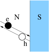
Figure 1: Andreev reflection by a superconductor (S). An incoming electron (e) in a normal metal (N) near the Fermi energy $E_{\rm F}$ is reflected as a hole (h) with opposite velocity.

Andreev reflection plays a central role in the description of hybrid nanostructures with both superconducting and normal components And64 . The process is illustrated in Fig. 1. When a negatively charged electron in the normal metal hits the interface with a superconductor, it is retroreflected into a positively charged hole. The superconductor acts as a charge-inverting mirror, which leads to a variety of intriguing effects in transport and spectroscopy of hybrid nanostructures Imry . Here, we show how Andreev reflection resonantly enhances the tunneling conductance through a quantum dot by orders of magnitude, when the dot is coupled to two superconductors with phase difference $\phi=\pi$ between their order parameters. The effect quickly disappears as $\phi$ is tuned away from resonance and might have applications in low-temperature current switching devices and magnetic flux “transistors”, where $\phi$ would be controlled by an external magnetic flux.

In a chaotic Andreev billiard, an impurity-free quantum dot coupled to one or more superconductors, Andreev reflection renders all orbits periodic near the Fermi level Kos95 . Periodic orbits consist of an electron and a hole retracing each other’s path, and therefore touching the superconductor at both ends. This fact suggests that the density of states of an Andreev billiard can be determined by Bohr-Sommerfeld quantization. For a single superconducting lead, this results in a density of states which is exponentially suppressed for low energies, on the scale of the Thouless energy $E_{\rm T,S}=\hbar/2\tau_{\rm D,S}$, where $\tau_{\rm D,S}$ is the average time between Andreev reflections Mel96 ; Sch99 . Simultaneously, one expects random matrix theory (RMT) to be valid for chaotic quantum dots BGS . RMT however leads to a different prediction, that a hard gap in the density of states opens up at an energy $E_{0}\simeq 0.6E_{\rm T,S}$Mel96 . It was realized in Ref. Lod98 that the discrepancy between the theories was not a short-coming in one of them but indicates that they have different regimes of validity. The crossover between the two regimes is determined by the Ehrenfest time, which is the time scale for an initially minimal wave packet to spread over the system. For a closed chaotic billiard of linear size $L_{\rm c}$ and Lyapunov exponent $\lambda$, the Ehrenfest time reads $\tau_{\rm E}=\lambda^{-1}\ln[k_{\rm F}L_{\rm c}]$, with the Fermi wavenumber $k_{\rm F}$ of the quasiparticles Sch05 .

RMT is valid in the universal regime of vanishing Ehrenfest time, $\tau_{\rm E}\ll\tau_{\rm D,S}$, while Bohr-Sommerfeld quantization gives a good description in the opposite semiclassical regime, $\tau_{\rm E}\gg\tau_{\rm D,S}$. Previous investigations of the crossover from the RMT regime to the semiclassical regime in Andreev billiards have considered the density of states in the presence of a single $s$-wave superconductor, focusing on the reduction of the excitation gap in the semiclassical regime, as well as its fluctuations Sch05 ; Ada02 ; Vav03 ; Sil03 ; Jac03 ; Goo03 ; Kor04 ; Goo05 ; Silv06 ; Mel97 ; Zho98 ; Tar01 . The Ehrenfest time effects are usually small and it takes a large computational effort to extract them numerically.

In this article we investigate transport via normal metallic leads through an Andreev billiard connected to two $\phi$-biased superconductors. The system we consider is shown in Fig. 2. A chaotic quantum dot with mean level spacing $\delta$ is coupled to two superconductors. The superconducting lead $1$ ($2$) has order parameter $\Delta_{0}e^{i\phi_{1}}$ ($\Delta_{0}e^{i\phi_{2}}$), and we take $\Delta_{0}\in{\cal R}$. One way to control the phase difference $\phi\equiv\phi_{1}-\phi_{2}$ is to have them form a loop, which one then threads with a magnetic flux $\Phi$ – this is sketched in Fig. 2. Alternatively, the phase difference can be generated by a supercurrent. In this case $\phi\equiv\phi_{1}-\phi_{2}=2\pi\Phi/\Phi_{0}$, in terms of the flux quantum $\Phi_{0}=h/2e$. Since any global phase can be gauged out, we set $\phi_{1}=\phi/2$ and $\phi_{2}=-\phi/2$. We assume that each superconducting lead has $N_{\rm S}$ channels connected to the quantum dot via tunnel contacts with tunnel probability $\Gamma_{\rm S}$. The average time $\tau_{\rm D,S}=\hbar/2E_{\rm T,S}$ between Andreev reflections is associated with the superconducting Thouless energy $E_{\rm T,S}=2N_{\rm S}\Gamma_{\rm S}\delta/4\pi$. Quasiparticle excitations have energy $E$ measured from the Fermi energy $E_{\rm F}$, with $|E|\ll\Delta_{0}$. Thus the quasiparticles cannot penetrate into the superconductors. We also assume $\Delta_{0}\ll E_{\rm F}$, in which case Andreev reflection perfectly retroreflects electrons into holes and vice versa, with a phase shift $-\pi/2\pm\phi_{i}$. At $\phi=0$, this Andreev phase shift is solely due to the penetration of the wavefunction into the superconductor. The additional phase shift $\pm\phi_{i}$ is due to the global phase of the superconductor at contact $i$, where the minus sign is for reflection from electron to hole, and the plus sign for reflection from hole to electron. We will refer to the quantum dot with two superconducting leads (but no normal lead) as the closed Andreev billiard. For the transport set-up we connect the quantum dot to two external normal leads through a tunnel contact with tunnel probability $\Gamma_{\rm N}$. The current is measured between the right (R) and left (L) lead, which both carry $N_{\rm N}$ transport channels.

The combination of Andreev and Ehrenfest physics in such an Andreev interferometer gives rise to an order-of-magnitude enhancement of the tunneling conductance when $\phi=\pi$. In the tunneling regime $\Gamma_{\rm N}\rightarrow 0$, the conductance is strongly affected by the density of states of the closed Andreev billiard. In the absence of superconductivity ($\Gamma_{\rm S}=0$) and for $\Gamma_{\rm N}N_{\rm N}\gtrsim 1$ (we restrict ourselves to that regime to avoid Coulomb blockade effects), the conductance is just the classical series conductance $G=G_{0}\Gamma_{\rm N}N_{\rm N}/2+{\cal O}(1),$ where $G_{0}=2e^{2}/h$ Bee97 . In contrast, we will see below that in the limit $\tau_{\rm E}/\tau_{\rm D}\sim 1$, and for well coupled superconductors, $\Gamma_{\rm S}\simeq 1$, the conductance at $\phi=\pi$ becomes $G\propto G_{0}N_{\rm N}$. We identify the mechanism behind this enhancement as macroscopic resonant tunneling through a large number of low-energy quasi-degenerate Andreev levels very close to the Fermi energy. Indeed, for $\phi=\pi$, all periodic trajectories touching both superconductors, irrespective of their lengths, contribute to the density of states at the Fermi energy in the semiclassical regime. Such a large effect is already clearly visible for moderate Ehrenfest time, in contrast to previous works which found rather small manifestations of Ehrenfest physics for larger $\tau_{\rm E}/\tau_{\rm D}$  Ada02 ; Vav03 ; Sil03 ; Jac03 ; Goo03 ; Kor04 ; Goo05 ; Silv06 . While similar behaviors were reported for cavities without transport Kad95 or internal Blom mode-mixing, this effect was not found in earlier analytical works on transport through chaotic Andreev interferometers Spi82 ; Zai94 ; Bee95 ; Kad99 .

\psfrag{Gn}{$\Gamma_{\rm N},N_{\rm N}$}\psfrag{Gs}{$\Gamma_{\rm S},N_{\rm S}$}\psfrag{R}{$R$}\psfrag{L}{$L$}\psfrag{P}{$\Phi$}\psfrag{phi1}{$-\phi/2$}\psfrag{phi2}{$\phi/2$}\psfrag{1}{$S_{1}$}\psfrag{2}{$S_{2}$}\includegraphics[width=227.62204pt]{fig2.eps}

Figure 2: Quantum dot doubly coupled to a superconducting ring. Both contact to the superconductor have $N_{\rm S}$ channels and tunneling probability $\Gamma_{\rm S}$. The flux threading the ring causes a phase difference $\phi=2\pi\Phi/\Phi_{0}$ between the two superconducting contacts. Transport through the structure is investigated between two external normal leads ($L$ and $R$), each carrying $N_{\rm N}$ transport channels, with tunnel contact of tunnel probability $\Gamma_{\rm N}$.

The paper is organized as follows. In section II we calculate the density of states of the closed Andreev billiard. We repeat previous results in the RMT limit and calculate the Bohr-Sommerfeld density of states as a function of $\phi$. We show that due to a special resonance condition, the density of states for phase differences close to $\pi$ has a large peak around the Fermi energy. We proceed with a calculation of the conductance in Section III. In the RMT limit we use Nazarov’s circuit theory Naz94 ; Arg96 . For weakly coupled normal leads, we find that the conductance is small, $\propto\Gamma_{\rm N}^{2}N_{\rm N}$, for $\phi\ll\pi$, while it reaches the classical series conductance for $\phi=\pi$, because of the disappearance of the gap in the density of states. In the semiclassical limit we employ a semiclassical trajectory-based method Jac06 ; Semicl ; Ada03 ; Bro06a ; Whi07 . We find that the large peak in the density of states at the Fermi level has its counterpart in the conductance, which is a factor $1/\Gamma_{\rm N}\gg 1$ larger than in the RMT limit. In section IV, numerical simulations confirm the validity of our analytical results.

II Spectrum of Andreev billiards

II.1 Random matrix theory

The density of states in the universal regime has been calculated in Refs. Mel96 ; Mel97 using RMT. We repeat the main steps of the calculation for $\Gamma_{\rm S}=1$, and refer the reader to Refs. Mel96 ; Fra96 for the calculation at arbitrary $\Gamma_{\rm S}$. At low excitation energy $E\ll\Delta_{0}$, the spectrum of Andreev billiards is most conveniently obtained from the low-energy effective Hamiltonian Fra96

$${\cal H} = \left(\begin{array}[]{cc}H&-\pi WW^{T}\\ -\pi WW^{T}&-H^{*}\end{array}\right)\,,$$ (1c)

$$W_{mn} = \delta_{mn}\left(\frac{M\delta}{\pi^{2}}\right)^{1/2},$$

$$m=1,2,\ldots M,\;\;\;\;\,n=1,2,\ldots 2N_{\rm S},$$

which is constructed from the quantum dot’s one-quasiparticle $M\times M$ Hamiltonian matrix $H$ and the projection matrix $WW^{T}$ giving the coupling between the quantum dot and the superconductors. We define a $2\times 2$ Green function $G(z)$ from the matrix Green function ${\cal G}(z)=\langle(z-{\cal H})^{-1}\rangle$

$$G=\left(\begin{array}[]{cc}G_{11}&G_{12}\\ G_{21}&G_{22}\end{array}\right)=\frac{\delta}{\pi}\left(\begin{array}[]{cc}{\rm Tr}{\cal G}_{11}&{\rm Tr}{\cal G}_{12}\\ {\rm Tr}{\cal G}_{21}&{\rm Tr}{\cal G}_{22}\end{array}\right),$$ (6)

from which the density of states reads

$$\rho_{\rm RMT}(E)=-\frac{2}{\delta}{\rm Im}[G_{11}(E+i0^{+})].$$ (7)

Here, $G_{11}$ is self-consistently determined by the equations

$$G_{11}(z)= -\frac{2\pi z}{N_{\rm S}\delta}\left(G_{12}^{2}(z)+\frac{G_{12}(z)}{\cos{(\phi/2)}}\right),$$ (8a)

$$G_{12}^{2}(z)= 1+G_{11}^{2}(z).$$ (8b)

For $\phi=0$, the density of states has a gap at an energy $E_{0}\approx 0.6E_{\rm T,S}$. The energy of the gap is reduced when $\phi$ is increased, closing at a value $\phi=\pi$, where one finds a flat density of states $\rho(E)=2/\delta$.

The theory of Refs. Mel96 ; Mel97 is only valid for energies larger than the level spacing $\delta$. For a phase difference $\phi=\pi$, the system belongs to the symmetry class CI of Ref. Zir97 , and the density of states reads

$$\rho(E)=\frac{\pi}{\delta}\int_{0}^{2\pi E/\delta}dtJ_{0}(t)J_{1}(t)/t,$$ (9)

with Bessel functions $J_{0}$ and $J_{1}$. This prediction retains its validity down to low excitations $E<\delta$. For energies $E\gg\delta$ (but still $E\ll\Delta_{0}$), Eq. (9) reduces to the mean field theory and gives $\rho(E)=2/\delta$, while for $E\lesssim\delta$ it predicts a linearly vanishing density of states $\rho(E)=\pi^{2}E/\delta$.

II.2 Semiclassical regime

The retroreflection at the superconductor makes all classical trajectories near the Fermi level periodic Kos95 . The elements of a periodic trajectory are an electron and a hole segment retracing each other, and touching a superconducting contact at both ends. The phase accumulated along a periodic orbit of period $T$ in one period consists of (i) the phase $2ET/\hbar$ acquired during the motion in the normal region and (ii) the phase shift acquired at the two Andreev reflections. This shift equals $-\pi$ if the two reflections take place at the same superconducting lead and $-\pi\pm\phi$ if they take place at different superconductors. Summing the different contributions and requiring that the phase accumulated in one period is a multiple of $2\pi$ leads to the Bohr-Sommerfeld quantization conditions

$$E_{n} = \pi\hbar(n+1/2)\,\Big{/}\,T,$$ (10a)

$$E_{n} = \pi\hbar(n+1/2+\phi/2\pi)\,\Big{/}\,T,$$ (10b)

$$E_{n} = \pi\hbar(n+1/2-\phi/2\pi)\,\Big{/}\,T.$$ (10c)

Eq. (10a) applies to trajectories touching the same superconductor twice, while Eqs. (10b) and (10c) to trajectories touching both superconductors, depending on whether the Andreev reflection from electron to hole takes place at the superconductor with phase $\phi/2$ [Eq. (10b)] or $-\phi/2$ [Eq. (10c)]. Assuming ergodicity, the corresponding trajectories have a weight $1/2$, $1/4$, $1/4$, leading to a mean density of states (see also Ref. Ihra01 for a single superconducting contact)

$$\rho_{\rm BS}(E)=N_{\rm S}\int_{0}^{\infty}dTP(T)\sum_{n}\left[\delta\left(E-[n+\frac{1}{2}]\frac{\pi\hbar}{T}\right)+\frac{1}{2}\delta\left(E-[n+\frac{1}{2}+\frac{\phi}{2\pi}]\frac{\pi\hbar}{T}\right)+\frac{1}{2}\delta\left(E-[n+\frac{1}{2}-\frac{\phi}{2\pi}]\frac{\pi\hbar}{T}\right)\right].$$ (11)

Here $P(T)$ is the classical distribution of return times to a superconducting contact. Inserting the chaotic distribution $P(T)=\exp{(-T/\tau_{\rm D,S})}\big{/}\tau_{\rm D,S}$ into Eq. (11) gives

$$\rho_{\rm BS}(u)= \frac{2\pi}{\delta}\frac{\cosh{\left(\frac{\phi}{2u}\right)}}{\sinh{\left(\frac{\pi}{u}\right)}u^{2}}\left(\pi\cosh{\left(\frac{\phi}{2u}\right)}\coth{\left(\frac{\pi}{u}\right)}-\phi\sinh{\left(\frac{\phi}{2u}\right)}\right),$$ (12)

with $u=E/E_{\rm T,S}$. For $\phi=0$ Eq. (12) reduces to the Bohr-Sommerfeld approximation of Refs. Mel96 ; Sch99 and the density of states is exponentially suppressed at low energies.

II.3 Comparison of the two regimes

Figure 3: Comparison of the density of states calculated from Bohr-Sommerfeld quantization and random matrix theory (RMT). The top panel is for a phase difference $\phi=0$, and the bottom panel for $\phi\approx\pi$.

The low energy approximation of Eq. (12) reads

$$\lim_{u\rightarrow 0}\rho_{\rm BS}(u)=\frac{2\pi}{\delta}\frac{e^{-(\pi-\phi)/u}(\pi-\phi)}{2u^{2}}.$$ (13)

For $\pi-\phi\ll 1$ this gives a sharply peaked function with a maximum value of $\rho_{BS}=\frac{4\pi}{e^{2}(\pi-\phi)}$ at energy $u=\frac{\pi-\phi}{2}$. In the limit $\phi\rightarrow\pi$ we find

$$\lim_{u\rightarrow 0}\lim_{\phi\rightarrow\pi}\rho_{\rm BS}(u)=\frac{2\pi}{\delta}\delta(u).$$ (14)

Eq. (14) predicts a number ${\cal O}[N_{\rm S}]$ of levels around $E=0$. The peculiar behavior at $\phi=\pi$ is due to the fact that the two quantization conditions (10b) and (10c) have solutions $E=0$ simultaneously for all trajectories, irrespective of their period.

Fig. 3 illustrates the predictions of the previous two paragraphs. In the RMT limit we combine the solution of Eqs. (8a) and (8b) with Eq. (7), while in the semiclassical limit we use Eq. (11). For $\phi=0$ (top panel), the density of states in the RMT and semiclassical limit are very similar. Both densities of states are suppressed at the Fermi energy, while they are restored to a value of $2/\delta$ at an energy scale set by $E_{\rm T,S}$. The main difference is in the way that $\rho$ is suppressed: a hard gap in the RMT limit vs. an exponential suppression for the semiclassical density of states.

In contrast, when $\phi\approx\pi$, the difference between RMT and Bohr-Sommerfeld predictions is huge. While in the RMT limit the density of states is flat [up to the minigap of order $\delta$ predicted by Eq.(9) which is not resolved in Fig. 3], it shows a large peak around the Fermi energy in the semiclassical limit. For $\phi=\pi$ the peak is described by a Dirac $\delta$-function (cf. Eq. (14)), which is why we show a density of states at a phase difference slightly different from $\pi$ in Fig. 3.

III Transport

III.1 Random matrix theory

\psfrag{N}{$N$}\psfrag{S}{$S$}\psfrag{1}{$1$}\psfrag{2}{$2$}\psfrag{3}{$3$}\psfrag{4}{$4$}\psfrag{5}{$5$}\psfrag{Nn}{$N_{\rm N},\Gamma_{\rm N}$}\psfrag{Ns}{$N_{\rm S},\Gamma_{\rm S}$}\includegraphics[width=71.13188pt]{fig4.eps}

Figure 4: Circuit for our system. We have two normal electrodes ($1,2$), two superconducting electrodes ($3,4$) and one internal junction, the chaotic cavity ($5$). The superconducting (normal) leads have $N_{\rm S}$ ($N_{\rm N}$) channels with transmission probability $\Gamma_{\rm S}$ ($\Gamma_{\rm N}$).

We use Nazarov’s circuit theory of Andreev conductance Naz94 to calculate the two-terminal conductance through the system shown in Fig. 2 (see also Ref. Arg96 ). The theory describes hybrid nanostructures in the same language as electrical circuits: i.e. their structure is reduced to internal junctions, normal/ superconducting external junctions (electrodes) and leads connecting the different elements. The leads are characterized by a set of transmission eigenvalues. The conductance between different electrodes is determined by a simple set of algebraic equations. As the energy dependence of the scattering matrix is neglected, the theory is valid for small temperatures and voltages. The superconductors have the same voltage. The results are valid to leading order in $\Gamma_{\rm S}N_{\rm S}$, $\Gamma_{\rm N}N_{\rm N}$.

Our system consists of two normal external junctions (denoted by indices $1,2$), two superconducting external junctions $3,4$ and one internal junction, the chaotic cavity $5$. This is illustrated in Fig. 4. The calculation of the conductance starts with the assignment of a complex amplitude $f_{k}$ to each junction. The amplitudes are somewhat analogous to voltages: if a junction $n$ is connected to a junction $m$ by a lead with a large conductance, then $f_{n}\rightarrow f_{m}$. The physical meaning of the amplitudes is the following: if electrons are injected into the $k^{\rm th}$ junction via an additional weakly coupled normal electrode, a beam of holes with intensity $|f_{k}|^{2}$ times that of the electron beam is retro-reflected into that probe. For the external junctions the value of the amplitudes is prescribed by the theory: for the normal external junctions $f_{1}$,$f_{2}=0$ and for the superconducting junctions $f_{3}=\exp{(-i\phi/2)}$, $f_{4}=\exp{(i\phi/2)}$. The amplitude $f_{5}$ can be found by the spectral current conservation rule Arg96 . One has $f_{5}=\tan(\theta_{5}/2)$, with $\theta_{5}$ to be determined by

$$\frac{\Gamma_{\rm S}N_{\rm S}}{\Gamma_{\rm N}N_{\rm N}}\cos{\frac{\phi}{2}}\cos{\theta_{5}}(1+\cos{\theta_{5}})\left(1+(1-\Gamma_{\rm N})\tan^{2}{\frac{\theta_{5}}{2}}\right)$$

$$=\sin\theta_{5}(2-\Gamma_{\rm S}+\Gamma_{\rm S}\sin{\theta_{5}}\cos{\frac{\phi}{2}}).\qquad$$ (15)

Once the complex amplitudes are known, the RMT-averaged conductance between junctions $1$ and $2$ is given by

$$\langle G\rangle/G_{0}=\frac{\Gamma_{\rm N}N_{\rm N}}{2}\frac{\cos{\theta_{5}}+\Gamma_{\rm N}\sin^{2}[\theta_{5}/2]}{(1-\Gamma_{\rm N}\sin^{2}[\theta_{5}/2])^{2}}.$$ (16)

The self-consistency equation (III.1) for $\theta_{5}$ combined with Eq. (16) determines the conductance. For ballistic leads ($\Gamma_{\rm N}=\Gamma_{\rm S}=1$) we reproduce the results of Ref. Bee95 .

Of most interest to us is the regime $\Gamma_{\rm N}\ll 1$ and $\Gamma_{\rm S}=1$, where we expect a strong connection between conductance and density of states. In the limit $\delta\phi=\pi-\phi\gg\Gamma_{\rm N}$, we use an expansion in terms of $\Gamma_{\rm N}$, while in the opposite limit, we first expand in the small parameter $\delta\phi$ . From Eqs. (III.1) and (16) we find, to leading order in $\Gamma_{\rm N}$,

$$\langle G\rangle/G_{0}=\left\{\begin{array}[]{cc}\Gamma_{\rm N}^{2}N_{\rm N}\left(1+\frac{N_{\rm N}}{N_{\rm S}}\frac{1+\cos{\frac{\phi}{2}}}{\cos{\frac{\phi}{2}}}\right)\Big{/}4,&\mbox{if}\hskip 2.84544pt\delta\phi\gg\Gamma_{\rm N},\\ \\ \Gamma_{\rm N}N_{\rm N}/2+{\cal O}(\delta\phi^{2}),&\mbox{if}\hskip 2.84544pt\delta\phi\ll\Gamma_{\rm N}.\end{array}\right.$$ (20)

The main feature of Eq. (20) is that, for $\phi=\pi$, one has the same conductance as a two-terminal quantum dot without superconductor. This result agrees with the density of states where the influence of the superconductors also disappears and the density of states becomes flat (bottom panel of Fig. 3). The minigap of magnitude $\delta$ is hardly resolved, due to the coupling to external leads and the associated broadening of levels. On the other hand, for $\phi\neq\pi$ the density of states is strongly suppressed at the Fermi level (top panel of Fig. 3) and we expect a conductance which is reduced due to the presence of the superconductors. Eq. (20) does indeed predict a conductance of order $\Gamma_{\rm N}^{2}$.

From Eq. (20) it follows that the crossover between the two limits occurs when $\delta\phi=\Gamma_{\rm N}N_{\rm N}/N_{\rm S}$. We now connect this to the density of states of the Andreev billiard. Taylor expanding Eqs. (7), (8a) and (8b) in $\delta\phi$ gives a gap in the density of states at an energy

$$E_{0}=\delta\phi\,E_{\rm T,S}=\delta\phi\,\frac{N_{\rm S}\,\delta}{2\pi}.$$ (21)

The density of states of the closed cavity is broadened due to the coupling to normal leads. The coupling to leads results in a non-hermitian Hamiltonian $H\rightarrow H-i\pi W_{\rm N}W_{\rm N}^{\dagger}$, with $H$ the Hamiltonian of the closed system and $W_{\rm N}$ an $M\times 2N_{\rm N}$ matrix describing the coupling to the normal leads Bee97 ; Iida90 . The $2N_{\rm N}\times 2N_{\rm N}$ matrix $W_{\rm N}^{\dagger}W_{\rm N}$ has eigenvalues $w=\Gamma_{\rm N}M\delta/4\pi^{2}+{\cal O}(\Gamma_{\rm N}^{2})$. For the broadening we need the eigenvalues of the $M\times M$ matrix $W_{\rm N}W_{\rm N}^{\dagger}$. Assuming that all levels in the dot are coupled to the leads in the same manner, we multiply $w$ by $2N_{\rm N}/M$ to estimate the broadening as $\delta E=2\pi wN_{\rm N}/M=\Gamma_{\rm N}N_{\rm N}\delta/2\pi$. Comparing this with Eq. (21) we find that $\delta E=E_{0}$ for $\Gamma_{\rm N}N_{\rm N}=N_{\rm S}\delta\phi$. This gives the crossover energy scale for Eqs. (20). We conclude that the conductance is not affected by the presence of the superconductors once the gap in the broadened density of states closes.

We finally comment on the effect of a finite tunnel barrier with $\Gamma_{\rm S}<1$ between the superconductor and normal metal. For $\Gamma_{\rm N}\ll 1$, Eq. (16) becomes

$$\langle G\rangle/G_{0}=\left\{\begin{array}[]{cc}\Gamma_{\rm N}^{2}N_{\rm N}\left(1+\frac{N_{\rm N}}{N_{\rm S,\rm eff}}\frac{1+\cos{\frac{\phi}{2}}}{\cos{\frac{\phi}{2}}}\right)\Big{/}4,&\mbox{if}\hskip 2.84544pt\delta\phi\gg\Gamma_{\rm N},\\ \\ \Gamma_{\rm N}N_{\rm N}/2+{\cal O}(\delta\phi^{2}),&\mbox{if}\hskip 2.84544pt\delta\phi\ll\Gamma_{\rm N}.\end{array}\right.$$ (25)

Here, $N_{\rm S,\rm eff}=c\,\Gamma_{\rm S}N_{\rm S}$ where $c\in(\frac{1}{2},1)$ is a numerical factor depending only weakly on $\phi$ and $\Gamma_{\rm S}$. A finite $\Gamma_{\rm S}$ thus reduces the number of effective superconducting channels to $N_{\rm S,{\rm eff}}$.

III.2 Semiclassical regime

The starting point of our semiclassical treatment is the two-terminal conductance through a metallic system in contact with superconductors (see Fig. 5) Lam93 ,

$$G/G_{0}=T_{RL}^{ee}+T_{RL}^{he}+2\frac{T_{LL}^{he}T_{RR}^{he}-T_{LR}^{he}T_{RL}^{he}}{T_{LL}^{he}+T_{RR}^{he}+T_{LR}^{he}+T_{RL}^{he}}.$$ (26)

We used the transmission probability for a quasi-particle of type $\alpha=e,h$ from the normal lead $i=L,R$ to a quasi-particle of type $\beta=e,h$ into the normal lead $j=L,R$,

$$T_{ji}^{\beta\alpha}=\sum_{m\in i;n\in j}|\tau^{\beta\alpha}_{n,j;m,i}|^{2}.$$ (27)

Here, $\tau^{\beta\alpha}_{n,j;m,i}$ gives the transmission amplitude from channel $m$ in lead $i$ to channel $n$ in lead $j$. Since we consider a symmetric configuration, where both normal leads carry the same number $N_{\rm N}$ of channels, all of them coupled to the cavity with the same tunnel probability $\Gamma_{\rm N}$, Eq. (26) simplifies to

$$\langle G\rangle/G_{0}=\langle T_{RL}^{ee}\rangle+\langle T_{LL}^{he}\rangle.$$ (28)

Eq. (28) gives the ensemble-averaged conductance to leading order in $\Gamma_{\rm N}\,N_{\rm N}\gg 1$.

\psfrag{Gamma}{\Large$\Gamma_{\rm N},N_{\rm N}$}\psfrag{gs1}{\Large$\gamma_{s1}$}\psfrag{gs2}{\Large$\gamma_{s2}$}\psfrag{gs3}{\Large$\gamma_{s3}$}\psfrag{gn}{\Large$\gamma_{\rm n}$}\psfrag{R}{\Large$R$}\psfrag{L}{\Large$L$}\psfrag{S1}{\Large$S_{1}$}\psfrag{S2}{\Large$S_{2}$}\psfrag{D1}{\Large$\Delta e^{-i\phi/2}$}\psfrag{D2}{\Large$\Delta e^{i\phi/2}$}\psfrag{Gammas}{\Large$\Gamma_{\rm S},N_{\rm S}$}\includegraphics[width=256.0748pt]{fig5.eps}

Figure 5: Schematic of the class I (blue) and class II (red) periodic orbits of the closed Andreev billiard, giving rise to macroscopic resonant tunneling at $\phi=\pi$ when the cavity is connected to external electrodes ($L$ and $R$).

To evaluate the resonant contributions to $\langle T_{RL}^{ee}\rangle$ and $\langle T_{LL}^{he}\rangle$, we follow the semiclassical approach of Ref. Jac06 (see also Refs. Semicl ; Ada03 ; Bro06a ; Whi07 ) Semiclassically, the transmission amplitudes read,

$$\tau^{\beta\alpha}_{n,j;m,i} = -(2\pi{\rm i}\hbar)^{-1/2}\!\int_{\rm i}\!\!{\rm d}y_{0}\int_{\rm j}\!{\rm d}y\sum_{\gamma}A_{\gamma}$$ (29)

$$\qquad\times\langle n|y\rangle\langle y_{0}|m\rangle\exp[{\rm i}S_{\gamma}/\hbar+{\rm i}\pi\mu_{\gamma}/2]\,,\qquad$$

where $|m\rangle$ is the transverse wavefunction of the $m^{\rm th}$ lead mode. This expression sums over all trajectories $\gamma$ (with classical action $S_{\gamma}$ and Maslov index $\mu_{\gamma}$) starting at $y_{0}$ on a cross-section of the injection ($i$) lead and ending at $y$ on the exit ($j$) lead, with even ($\alpha=\beta$) or odd ($\alpha\neq\beta$) number of Andreev reflections. The transmission probabilities are then given by a double sum over trajectories. After the semiclassical approximation that $\sum_{n}\langle y^{\prime}|n\rangle\langle n|y\rangle\simeq\delta(y^{\prime}-y)$ Jac06 one has

$$T_{ji}^{\beta\alpha} = \frac{1}{2\pi\hbar}\int_{i}{\rm d}y_{0}\int_{j}{\rm d}y_{0}^{\prime}\sum_{\gamma 1,\gamma 2}A_{\gamma 1}A_{\gamma 2}^{*}\exp[i\delta S/\hbar]\,.\qquad$$ (30)

This expression sums over all pairs of classical trajectories $\gamma 1$ and $\gamma 2$ with fixed endpoints $y_{0}$ and $y_{0}^{\prime}$, which convert an $\alpha$ quasiparticle into a $\beta$ quasiparticle. The phase $\delta S=S_{\gamma 1}-S_{\gamma 2}$ gives the difference in action phase accumulated along $\gamma 1$ and $\gamma 2$. In the presence of tunnel barriers, the stability amplitudes $A_{\gamma}$ are given by Whi07 ; Cou92

$$A_{\gamma}=B_{\gamma}\,t_{i}t_{j}\,\prod_{k}[r_{k}]^{l_{\gamma}(k)},$$ (31)

where $l_{\gamma}(k)$ gives the number of times that $\gamma$ is reflected back into the system from the tunnel barrier at $k=L,R,S_{1},$ and $S_{2}$, the transmission and reflection amplitudes satisfy $|t_{i}|^{2}=(1-|r_{i}|^{2})=\Gamma_{\rm N,S}$ (for $i=L,\,R,\,S_{1},$ or $S_{2}$), and $B_{\gamma}^{2}=(dp_{y_{0}}/dy)_{\gamma}$ measures the rate of change of the initial momentum $p_{y_{0}}$ as the exit position $y$ of $\gamma$ is changed, for a fixed sequence of transmissions and reflections at the tunnel barriers.

There are four types of trajectories to consider:

(i) paths that do not touch the superconductors,

(ii) paths that hit one of the superconductor once,

(iii) paths that hit the same superconductor twice,

(iv) paths that hit both superconductors.

Trajectories of type (iv) are flux-dependent. They are depicted in Fig. 5, and it turns out that they are the ones giving rise to macroscopic resonant tunneling. Our semiclassical investigations focus on those paths.

We use Eqs. (30) and (31) to evaluate the dominant semiclassical contributions to Eq. (28). We subdivide the relevant trajectories into class I trajectories, contributing to $\langle T_{LL}^{he}\rangle$ (blue trajectory on Fig.5), and class II trajectories, contributing to $\langle T_{RL}^{ee}\rangle$ (red trajectory on Fig.5).

Class I trajectories are made of the following sequence

$$\gamma_{I}^{(p)}=\gamma^{(e)}_{s1}+\gamma^{(h)}_{s1}+p\times\left[\gamma^{(h)}_{s3}+\gamma^{(e)}_{s3}+\gamma^{(e)}_{s1}+\gamma^{(h)}_{s1}\right],$$ (32)

where $s1$ and $s3$ can be interchanged, and $p=0,1,2,\ldots$ These trajectories undergo $2p+1$ Andreev reflections and $2p$ reflections at tunnel barriers caveat . They accumulate an action phase

$$S_{\gamma,I}=p(-\pi+\phi+E\,t_{\ell\rm,I})+2\,E\,t_{\gamma_{s1}}-(\pi/2-\phi/2).$$ (33)

One should substitute $\phi\rightarrow-\phi$ when interchanging segments $s1$ and $s3$, though the relative sign between $\pi$ and $\phi$ does not affect the final result. Here, $t_{\ell\rm,I}$ gives the duration of the loop [the sequence between bracket in Eq. (32)] and $t_{\gamma_{s1}}$ is the duration of the segment $\gamma_{s_{1}}$ as shown on Fig. 5. Class II trajectories split into two subclasses, defined by the following two sequences

$$\gamma_{IIa}^{(p)} = \gamma^{(e)}_{n}$$

$$+ p\times\left[\gamma^{(e)}_{s2}+\gamma^{(h)}_{s2}+\gamma^{(h)}_{n}+\gamma^{(h)}_{s1}+\gamma^{(e)}_{s1}+\gamma^{(e)}_{n}\right]\,,$$

$$\gamma_{IIb}^{(p)} = \gamma^{(e)}_{s1}+\gamma^{(h)}_{s1}+\gamma^{(h)}_{n}+\gamma^{(h)}_{s2}+\gamma^{(e)}_{s2}$$

$$+ p\times\left[\gamma^{(e)}_{n}+\gamma^{(e)}_{s1}+\gamma^{(h)}_{s1}+\gamma^{(h)}_{n}+\gamma^{(h)}_{s2}+\gamma^{(e)}_{s2}\right]\,.$$

They undergo $2p$ (IIA) and $2p+2$ (IIb) Andreev reflections, $4p$ (IIa) and $4p+2$ (IIb) reflections at tunnel barriers caveat , and accumulate action phases

$$S_{\gamma,IIa} = p(-\pi-\phi+E\,t_{\ell\rm,IIa})+(E_{\rm F}+E)\,t_{\gamma_{n}},$$ (35a)

$$S_{\gamma,IIb} = p(-\pi+\phi+E\,t_{\ell\rm,IIb})-(E_{\rm F}-E)\,t_{\gamma_{n}}$$ (35b)

$$+2E\,(t_{\gamma_{s1}}+t_{\gamma_{s2}})-(\pi-\phi).$$

Here $t_{\ell\rm,IIa}$ and $t_{\ell\rm,IIb}$ give the duration of the Andreev loops [the two sequences between bracket in Eqs. (34)]. We already see that at $E=0$ and $\phi=\pi$, the phase difference accumulated by any two members (with different $p$) of a given family vanishes, so that all pair of trajectories within a given family resonate. There is however no resonance between members of different families.

In normal chaotic billiards, the stability $B_{\gamma}^{2}$ of periodic orbits decreases exponentially with the number of times the orbit is traveled Haake-book . The situation is fundamentally different in presence of superconductivity, where Andreev reflections refocus the dynamics. The stability of a trajectory is then only given by the product of the stabilities along the primitive segments, independent of $p$. We will take these primitive segments as $\gamma_{s1}$ and $\gamma_{s3}$ for class I, $\gamma_{s1}$, $\gamma_{n}$ and $\gamma_{s2}$ for class II, keeping in mind, however, that the contributions arising from the trajectories of class I and IIa with $p=0$ are more stable than those with $p\geq 1$, because they do not travel on $\gamma_{s3}$ (class I) nor on $\gamma_{s1}$ and $\gamma_{s2}$ (class IIa). Their contribution is thus underestimated in our approach, and our final results, Eqs. (III.2) and (III.2), underestimate the conductance by a subdominant correction.

This enhanced stability applies to trajectories whose Andreev loop is shorter than twice the Ehrenfest time, i.e. the time beyond which an initially narrow wavepacket can no longer fit inside a superconducting lead Lod98 ; Jac03 ; Vav03 . The relative measure of trajectories of class I ($P_{I}$) and II ($P_{II}$) is thus

$$P_{I}(\tau_{\rm E}/\tau_{\rm D,S}) = \tau_{\rm D,S}^{-2}\int_{0}^{\tau_{\rm E}}{\rm d}t_{s1}\int_{0}^{\tau_{\rm E}-t_{s1}}{\rm d}t_{s3}\,\exp[-(t_{s1}+t_{s3})/\tau_{\rm D,S}]=1-[1+\tau_{\rm E}/\tau_{\rm D,S}]\,\exp[-\tau_{\rm E}/\tau_{\rm D,S}],$$ (36a)

$$P_{II}(\tau_{\rm E}/\tau_{\rm D,S}) = \tau_{\rm D,S}^{-3}\int_{0}^{\tau_{\rm E}}{\rm d}t_{s1}\int_{0}^{\tau_{\rm E}-t_{s1}}{\rm d}t_{n}\int_{0}^{\tau_{\rm E}-t_{s1}-t_{n}}{\rm d}t_{s2}\,\exp[-(t_{s1}+t_{n}+t_{s3})/\tau_{\rm D,S}]$$ (36b)

$$= 1-[1+\tau_{\rm E}/\tau_{\rm D,S}+(\tau_{\rm E}/\tau_{\rm D,S})^{2}/2]\,\exp[-\tau_{\rm E}/\tau_{\rm D,S}]\,.$$

We are now ready to evaluate the dominant contributions to conductance close to resonance. We focus on the low-temperature regime with $E=0$. We start from Eq. (30) and pair trajectories by class, noting that for a given class, all trajectories have the same stability but differ only by the number of Andreev reflections and normal reflections at the contacts to the normal leads, as well as by the different action phases they accumulate along their Andreev loop. The sum over classes is then represented by a sum over primitive trajectories, and we perform the substitution

$$\sum_{\gamma 1,\gamma 2}A_{\gamma 1}A_{\gamma 2}^{*}\;[\dots]_{\gamma 1,\gamma 2}\;\longrightarrow\;\Gamma_{\rm N}^{2}\sum_{\gamma={\rm primitive}}B_{\gamma}^{2}\sum_{p,p^{\prime}=0}^{\infty}(1-\Gamma_{\rm N})^{a(p+p^{\prime})}\,\Gamma_{\rm S}^{p+p^{\prime}+c}\;[\dots]_{\gamma,p,p^{\prime}}\,.$$ (37)

The exponents $a=1$, $b=0$ and $c=1$ for class I, $a=2$, $b=0$ and $c=0$ for class IIa and $a=2$, $b=2$ and $c=2$ for class IIb are determined by the number of Andreev and normal reflections in Eqs. (32) and (34). Reflection phases do not appear because each time an electron is reflected at a tunnel barrier, a hole is reflected later. The argument in the double sum over $p$ and $p^{\prime}$ in Eq. (37) has to be multiplied by the $p$-$p^{\prime}$–dependent Andreev phase. The double sum over $p$ and $p^{\prime}$ is easily resummed,

$$\sum_{p,p^{\prime}=0}^{\infty} (1-\Gamma_{\rm n})^{a(p+p^{\prime})+b}\;\Gamma_{\rm s}^{p+p^{\prime}+c}\;e^{i(p-p^{\prime})(\phi-\pi)}=$$

$$\frac{\Gamma_{\rm S}^{c}\;(1-\Gamma_{\rm N})^{b}}{1-2\,\Gamma_{\rm S}\,(1-\Gamma_{\rm N})^{a}\cos[\pi-\phi]+\Gamma_{\rm S}^{2}\,(1-\Gamma_{\rm N})^{2a}}.$$

We next evaluate $\sum_{\gamma}B_{\gamma}^{2}$ by relating it to classical transmission probabilities Jac06 . Because the sum runs over primitive trajectories whose stability is given by their electronic (or hole) component alone, one considers that the cavity is opened to four normal leads. The sum runs over all trajectories such as those sketched in Fig. 6. For class I, these trajectories are made up of two legs, both of them starting at $y_{0}$ on the $L$ lead, and we write $\sum B_{\gamma}^{2}=\sum_{\gamma 1,\gamma 3}B_{\gamma 1}^{2}B_{\gamma 3}^{2}$. The leg $\gamma 1$ makes a normal angle $\theta_{0}$ with respect to the normal to a cross-section of $L$ and ends up in lead $S_{1}$, while $\gamma 3$ makes a normal angle $\theta_{0}^{\prime}=-\theta_{0}$ and goes to lead $S_{2}$. Both incidence position and angle on $S_{1}$ and $S_{2}$ have to be integrated over.

We define $P({\bf Y},{\bf Y}_{0};t)\delta y\delta\theta\delta t$ as the classical probability to go from an initial position and momentum angle ${\bf Y}_{0}=(y_{0},\theta_{0})$ on a lead to within $(\delta y,\delta\theta)$ of ${\bf Y}=(y,\theta)$ on another lead, in a time within $\delta t$ of $t$. The sum over all primitive trajectories of class I can then be rewritten as

$$\sum_{\gamma,{\rm primitive}}\!B_{\gamma}^{2} = \!\!p_{\rm F}\int_{0}^{\tau_{\rm E}}\!{\rm d}t_{s1}\int_{0}^{\tau_{\rm E}-t_{s1}}{\rm d}t_{s3}\;\int_{-\pi/2}^{\pi/2}{\rm d}\theta_{0}{\rm d}\theta_{0}^{\prime}$$ (39)

$$\times \int_{S1}{\rm d}y_{s1}\int_{S2}{\rm d}y_{s3}\int_{-\pi/2}^{\pi/2}{\rm d}\theta_{s1}{\rm d}\theta_{s2}$$

$$\times \;P({\bf Y}_{s1},{\bf Y}_{0};t_{s1})\,P({\bf Y}_{s3},{\bf Y}_{0};t_{s3})$$

$$\times \cos\theta_{0}\,\cos\theta_{0}^{\prime}\,\delta(\theta_{0}+\theta_{0}^{\prime})\,\delta(y_{0}-y_{0}^{\prime}).$$

The factor $p_{\rm F}\cos\theta_{0}$ measures the injected current, and since electrons are reflected (and not injected) at the $L$ tunnel barrier, one has an additional $\cos\theta_{0}^{\prime}$ (instead of $p_{\rm F}\cos\theta_{0}^{\prime}$). For a given cavity, $P$ is a sum of $\delta$-functions over all possible classical trajectories. Instead we consider the distribution averaged over a mesoscopic ensemble of similar cavities or a small energy interval. This gives a smooth function

$$\langle P({\bf Y}_{si},{\bf Y};t)\rangle=\frac{\tau_{\rm D,S}^{-1}\,\cos\theta_{si}}{4(\Gamma_{\rm N}W_{\rm N}+\Gamma_{\rm S}W_{\rm S})}\;\exp[-t/\tau_{\rm D,S}]\,,$$ (40)

where $W_{\rm N,S}=N_{\rm N,S}\pi/k_{\rm F}$ gives the width of the normal and superconducting leads. We insert (40) into (39), and perform the integrals. Combining the result with Eqs. (30), (37) and (III.2) delivers the resonant semiclassical contribution to $T_{LL}^{he}$,

$$\langle T_{LL}^{he}\rangle_{\rm r} = \frac{\pi\Gamma_{\rm N}^{2}N_{\rm N}}{4}\left(\frac{N_{\rm S}}{2\Gamma_{\rm N}N_{\rm N}+2\Gamma_{\rm S}N_{\rm S}}\right)^{2}$$

$$\times \Big{(}1-(1+\tau_{\rm E}/\tau_{\rm D,S})\exp[-\tau_{\rm E}/\tau_{\rm D,S}]\Big{)}$$

$$\times \frac{\Gamma_{\rm S}}{1-2\,\Gamma_{\rm S}\,(1-\Gamma_{\rm N})\cos[\pi-\phi]+\Gamma_{\rm S}^{2}\,(1-\Gamma_{\rm N})^{2}}\,.$$

\psfrag{g1}{\Large$\gamma_{1}$}\psfrag{gn}{\Large$\gamma_{n}$}\psfrag{g3}{\Large$\gamma_{2}$}\psfrag{g2}{\Large$\gamma_{3}$}\psfrag{R}{\Large$R$}\psfrag{S1}{\Large$S_{1}$}\psfrag{S2}{\Large$S_{2}$}\psfrag{L}{\Large$L$}\psfrag{ts1}{\Large$\theta_{s1}$}\psfrag{ts2}{\Large$\theta_{s2}$}\psfrag{t1}{\Large$\theta_{1}$}\psfrag{-t1}{\Large$-\theta_{1}$}\psfrag{t0}{\Large$\theta_{0}$}\psfrag{-t0}{\Large$-\theta_{0}$}\psfrag{y0}{\Large$y_{0}$}\psfrag{ys1}{\Large$y_{s1}$}\psfrag{ys2}{\Large$y_{s2}$}\includegraphics[width=241.84842pt]{fig6a.eps}

\psfrag{g1}{\Large$\gamma_{1}$}\psfrag{gn}{\Large$\gamma_{n}$}\psfrag{g3}{\Large$\gamma_{2}$}\psfrag{g2}{\Large$\gamma_{3}$}\psfrag{R}{\Large$R$}\psfrag{S1}{\Large$S_{1}$}\psfrag{S2}{\Large$S_{2}$}\psfrag{L}{\Large$L$}\psfrag{ts1}{\Large$\theta_{s1}$}\psfrag{ts2}{\Large$\theta_{s2}$}\psfrag{t1}{\Large$\theta_{1}$}\psfrag{-t1}{\Large$-\theta_{1}$}\psfrag{t0}{\Large$\theta_{0}$}\psfrag{-t0}{\Large$-\theta_{0}$}\psfrag{y0}{\Large$y_{0}$}\psfrag{ys1}{\Large$y_{s1}$}\psfrag{ys2}{\Large$y_{s2}$}\includegraphics[width=241.84842pt]{fig6b.eps}

Figure 6: The effective four-terminal cavity used in the calculation of $\sum B_{\gamma}^{2}$, and the geometry of class I (top panel) and class II (bottom panel) trajectories.

The semiclassical contribution to $T_{RL}^{ee}$ arises from class II trajectories. The geometry is detailed in Fig. 6, and a similar calculation as above delivers

$$\langle T_{RL}^{ee}\rangle_{\rm r} = \frac{\pi^{2}\Gamma_{\rm N}^{2}\,N_{\rm N}^{2}}{8N_{\rm S}}\left(\frac{N_{\rm S}}{2\Gamma_{\rm N}N_{\rm N}+2\Gamma_{\rm S}N_{\rm S}}\right)^{3}$$

$$\times \Big{(}1-(1+\tau_{\rm E}/\tau_{\rm D,S}+\tau_{\rm E}^{2}/2\tau_{\rm D,S}^{2})\exp[-\tau_{\rm E}/\tau_{\rm D,S}]\Big{)}$$

$$\times \frac{1+\Gamma_{\rm S}^{2}\,(1-\Gamma_{\rm N})^{2}}{1-2\,\Gamma_{\rm S}\,(1-\Gamma_{\rm N})^{2}\cos[\pi-\phi]+\Gamma_{\rm S}^{2}\,(1-\Gamma_{\rm N})^{4}}.$$

The semiclassical contribution to the conductance is given by the sum of Eqs. (III.2) and (III.2). It clearly exhibits the functional dependence of resonant tunneling, where the resonance is however always at the Fermi level, and is achieved by setting the phase difference between the two superconductors at $\phi=\pi$. This resonance condition is the same for all semiclassical contributions we just discussed. This is why the resonance is macroscopic, giving a conductance $G\propto N_{\rm N}$ and not of order one, as is usually the case for resonant tunneling. We also see that the effect disappears if the superconductors are poorly connected to the normal cavity, $\Gamma_{\rm S}\rightarrow 0$, as should be.

Comparing Eqs. (III.2) and (III.2) to Eq. (20) we see that semiclassical contributions matter only close to resonance. In the tunneling regime, they increase the conductance by a factor $\propto\Gamma_{\rm N}^{-1}$, from $G(\pi)/G_{0}\propto\Gamma_{\rm N}N_{\rm N}$ to $G(\pi)/G_{0}\propto N_{\rm N}$, resulting in a peak-to-valley ratio of the conductance $G(\phi=\pi)/G(\phi=0)\propto\Gamma_{\rm N}^{-2}$. In most instances, $\langle T_{LL}^{eh}(\pi)\rangle_{\rm r}\gg\langle T_{RL}^{ee}(\pi)\rangle_{\rm r}$, and the sharpness of the resonance peak, measured by its width at half height, is proportional to $\Gamma$.

IV Numerical simulations

We compare our theory with numerical simulations on a quantum mechanical model of the Andreev billiard, the Andreev kicked rotator Jac03 .

IV.1 The Andreev kicked rotator

One-dimensional maps give a stroboscopic description of dynamical systems. An example is the kicked rotator, describing the dynamics of a particle confined to a circle which is kicked periodically in time with period $\tau_{0}$ and a kicking strength depending on its position Sch05 . The quantized version of this map is characterized by its Floquet operator, the unitary operator giving the time-evolution from one kick to the next, i.e. from time $t$ to $t+\tau_{0}$. We represent the Floquet operator as a $M\times M$ matrix with matrix elements (from now on we measure times in units of $\tau_{0}\equiv 1$)

$$F_{nm} = e^{-(i\pi/2M)(n^{2}+m^{2})}(UQU^{\dagger})_{nm},$$ (43a)

$$U_{nm} = M^{-1/2}e^{(2\pi i/M)nm},$$ (43b)

$$Q_{nm} = \delta_{nm}e^{-(iMK/2\pi)\cos(2\pi n/M)}.$$ (43c)

Here $K$ is the kicking strength. For $K\gtrsim 7$ the classical dynamics is chaotic, with classical Lyapunov exponent $\lambda\simeq\ln[K/2]$. The eigenvalues of $F$ are $e^{i\epsilon_{m}}$ ($m=1\ldots M$), and the quasi-energies $\epsilon_{m}$ of the closed system (without any leads) have an average level spacing $\delta=2\pi/M$. The dynamics of the electron is determined by $F$, while the time evolution of holes is given by $F^{*}$.

The kicked rotator model describes a closed system. We open it by inserting leads in a subspace of the Hilbert space, parametrized by the indices $\{m_{1},m_{2},\ldots m_{2N_{\rm N}}\}$ for the normal leads and $\{l_{1},l_{2},\ldots l_{2N_{\rm S}}\}$ for the superconducting leads. The coupling to the leads is described by a $2N_{\rm N}\times M$ ($2N_{\rm S}\times M$) projection matrix $P_{\rm N}$ ($P_{\rm S}$) with matrix elements

$$[P_{\rm N}]_{nm} =\left\{\begin{array}[]{ll}\sqrt{\Gamma_{\rm N}}&\mbox{if\,}m=n\in\{m_{1},\ldots m_{2N_{\rm N}}\},\\ 0&\mbox{otherwise,}\end{array}\right.$$ (44c)

$$[P_{\rm S}]_{nm} =\left\{\begin{array}[]{ll}\sqrt{\Gamma_{\rm S}}&\mbox{if\,}m=n\in\{l_{1},\ldots l_{2N_{\rm S}}\},\\ 0&\mbox{otherwise.}\end{array}\right.$$ (44f)

The average time between Andreev reflections equals $\tau_{\rm D,S}=M/2\Gamma_{\rm S}N_{\rm S}$. In our numerical investigations we restrict ourselves to $\Gamma_{\rm S}=1$. The Ehrenfest time of the closed Andreev billiard reads $\tau_{\rm E}=\lambda^{-1}\ln{(N_{\rm S}^{2}/M)}$ Jac03 ; Vav03 .

We perform two sets of simulations, the first is devoted to the spectrum of a closed Andreev billiard, the second to the conductance through a chaotic Andreev interferometer.

IV.1.1 The closed Andreev kicked rotator

Both electrons and holes have an energy near the Fermi energy, and therefore we assume that Andreev reflection is perfectly retroreflecting. The Floquet matrix of the Andreev billiard is then

$${\cal F}={\cal P}_{S}\,\left(\begin{array}[]{cc}F&0\\ 0&F^{*}\end{array}\right)\,,$$ (47)

with

$${\cal P}_{S}=\left(\begin{array}[]{cc}1-P_{S}^{T}P_{S}&-iP_{S}^{T}e^{i\Phi}P_{S}\\ -iP_{S}^{T}e^{-i\Phi}P_{S}&1-P_{S}^{T}P_{S}\end{array}\right).$$ (50)

The coupling between electrons and holes is modelled by ${\cal P}_{S}$, which induces Andreev reflection for electron or holes touching the superconducting leads, i.e. induces transitions between the components $\{l_{1},\ldots l_{2N_{\rm S}}\}$ of the wavefunction in the two quasiparticle sectors. The phase difference between the two superconductors is contained in the $2N_{\rm S}\times 2N_{\rm S}$ matrix $\Phi$, with elements $\delta_{nm}\phi/2$, for $n\leq N_{\rm S}$ and $-\delta_{nm}\phi/2$ for $n>N_{\rm S}$. The matrix ${\cal F}$ can be diagonalized efficiently using the Lanczos technique in combination with the Fast-Fourier-Transform algorithm Ket99 . This allows to reach the large system sizes needed to explore the regime of finite Ehrenfest time.

IV.1.2 The kicked Andreev interferometer

We first write the $(2N_{\rm N}+2N_{\rm S})\times(2N_{\rm N}+2N_{\rm S})$ energy-dependent scattering matrix of our four-terminal structure (without superconductor). It is related to the Floquet operator via Fyo00

$$S(\epsilon)=-(1-PP^{T})^{1/2}+P\frac{1}{e^{-i\epsilon}-{F}(1-P^{T}P)}FP^{T}.$$ (51)

The $(2N_{\rm S}+2N_{\rm N})\times M$ coupling matrix

$$P=\left(\begin{array}[]{cc}P_{\rm N}&0\\ 0&P_{\rm S}\end{array}\right),$$ (54)

describes coupling to all four leads. The four-terminal scattering matrix $S$ is made of sixteen sub-blocks $S_{ij}$, where the subindices $i,j=L$, $R$, $S1$ and $S2$ label either normal or superconducting terminals. From these sub-blocks, the exact expression for the conductance, Eq. (26), can be computed, following Ref. Bee95 . The transmission amplitudes giving the probabilities in Eq. (27) can be written as

$$\tau^{\rm ee}=a-b\,\Omega c^{\ast}\Omega^{\ast}(1+c\,\Omega c^{\ast}\Omega^{\ast})^{-1}d,$$ (55a)

$$\tau^{\rm he}=-{\rm i}b^{\ast}\Omega^{\ast}(1+c\,\Omega c^{\ast}\Omega^{\ast})^{-1}d,$$ (55b)

in terms of the matrices

$$a={\left(\begin{array}[]{cc}S_{L,L}&S_{L,R}\\ S_{R,L}&S_{R,R}\end{array}\right)},\;\;\;\;\;\;\;\;\;b={\left(\begin{array}[]{cc}S_{L,S1}&S_{L,S2}\\ S_{R,S1}&S_{R,S2}\end{array}\right)},$$

$$c={\left(\begin{array}[]{cc}S_{S1,S1}&S_{S1,S2}\\ S_{S2,S1}&S_{S2,S2}\end{array}\right)},\;\;\;\;d={\left(\begin{array}[]{cc}S_{S1,L}&S_{S1,R}\\ S_{S2,L}&S_{S2,R}\end{array}\right)},$$

$$\Omega={\left(\begin{array}[]{ll}{\rm e}^{-{\rm i}\phi/2}&0\\ 0&{\rm e}^{{\rm i}\phi/2}\end{array}\right)}.$$

For numerical stability and efficiency, the transmission matrices $\tau$ of Eqs. (55) are constructed from self-consistent linear equations for the output amplitudes as a function of unity input on each $N_{\rm N}$ channel, one at a time, and not via direct inversion.

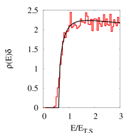
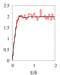
Figure 7: Left panel: density of states for the Andreev kicked rotator with $\phi=0$, $M=2048$, $N_{\rm S}=25$, $K=147$, $\Gamma_{\rm S}=1$. The solid line gives the prediction of Eqs. (7) and (8). Data are averaged over $50$ different lead positions. Right panel: density of states for the Andreev kicked rotator with $\phi=\pi$, $M=2048$, $N_{\rm S}=25$, $\Gamma_{\rm S}=1$. The solid line gives the prediction of Eq. (9). Data are averaged over $50$ different lead positions and $50$ values of the kicking strength $K\in[144.5,147.5]$

IV.2 Numerics in the universal regime

We start with a comparison of the analytical predictions of RMT with numerical results, by choosing the parameters of the Andreev kicked rotator in such a way that $\tau_{\rm E}\ll\tau_{\rm D,S}$. In Fig. 7 we show the density of states for $\phi=0$ and $\phi=\pi$. We compare our results with the theoretical predictions of Eqs. (7) and (8) for $\phi=0$, while for $\phi=\pi$ we use Eq. (9). In both cases we find perfect agreement between numerics and RMT predictions.

We next turn our attention to the conductance. We choose an Andreev billiard with the same parameters as in Fig. 7, but couple it to normal leads. The conductance as a function of the phase difference is shown in Fig. 8. The numerical results, for several values of the parameters $\Gamma_{\rm N}$ and $N_{\rm N}$ (characterizing the normal leads), are compared with the circuit theory prediction of Eqs. (III.1) and  (16). The agreement is excellent. In the tunneling limit $\Gamma_{\rm N}\rightarrow 0$ the conductance is strongly suppressed for $\phi\neq\pi$ while it is restored to its value in absence of superconductor when $\phi=\pi$, as predicted by Eq. (20).

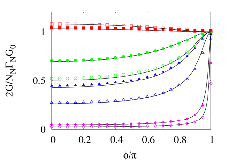
Figure 8: Conductance of the Andreev kicked rotator as a function of the phase difference $\phi$ between the two superconductors. For all curves $M=2048$, $N_{\rm S}=25$, $K=147$. The closed symbols correspond to $N_{\rm N}=100$ and the open symbols to $N_{\rm N}=50$, with $\Gamma_{\rm N}=1$ (squares), $\Gamma_{\rm N}=0.2$ (circles), $\Gamma_{\rm N}=0.1$ (triangles) and $\Gamma_{\rm N}=0.01$ (diamonds). The solid lines are the relevant predictions from circuit theory. Every data point is an average over $200$ realizations.

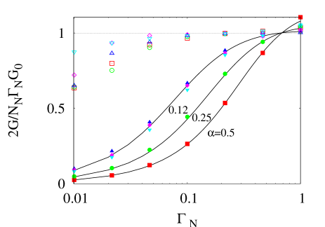
Figure 9: Conductance of the Andreev kicked rotator as a function of $\Gamma_{\rm N}$ for $K=147$, $M=2048$, $\Gamma_{\rm S}=1$, at $\phi=0$ (closed symbols) and $\phi=\pi$ (open symbols), and $N_{\rm N}/N_{\rm S}=100/50$ (squares), $100/25$ (circles), $100/12$ (upward pointing triangles), $200/25$ (diamonds) and $400/50$ (downward pointing triangles). Every data point is an average over $50$ realizations. The solid lines are the predictions from circuit theory for $\phi=0$ and $\alpha=N_{\rm S}/N_{\rm N}=0.5,0.25$, and $\alpha=0.12$, while the dashed line corresponds to $\phi=\pi$.

In Fig. 9, we show the conductance as a function of $\Gamma_{\rm N}$, both for $\phi=0$ and $\phi=\pi$. For $\phi=0$ the circuit theory of Eqs. (III.1) and (16) (solid lines) predict a curve that depends only on the ratio $\alpha\equiv N_{\rm S}/N_{\rm N}$. The numerical data line up on the analytical curves. For $\phi=\pi$ the analytical prediction of circuit theory coincides with the conductance of the billiard in the absence of superconductors i.e. $G/G_{0}=\Gamma_{\rm N}N_{\rm N}/2$. As $\Gamma_{\rm N}N_{\rm N}$ is reduced, however, the data deviate from this prediction. We attribute this to the fact that the circuit theory results are accurate to leading order in $\Gamma_{\rm N}N_{\rm N}$ only. This argument is corroborated by the fact that the data for the largest $N_{\rm N}$ remain close to the circuit theory prediction down to lower values of $\Gamma_{\rm N}$.

\psfrag{j=p}{\color[rgb]{1,0,0} \large$\phi=\pi$}\psfrag{j=0}{\large$\phi=0$}\psfrag{Andreev gap}{Andreev gap}\includegraphics[width=213.39566pt]{fig10.eps}

Figure 10: Transmission as a function of the normalized excitation energy $E/E_{\rm T,S}$ for $M=2048$, $N_{\rm N}=100$, $K=147$, $\Gamma_{\rm N}=0.05$, at $\phi=0$ (black symbols) and $\phi=\pi$ (red symbols) for $N_{\rm S}=25$ (triangles), 50 (diamonds), 100 (squares) and 200 (circles). The black curve shows the universal conductance at $\phi=\pi$ for $E=0$.

We next present in Fig. 10 data for the conductance at finite excitation energy. For $\phi=\pi$, the conductance stays at its universal, $E=0$ value, $G=\Gamma_{\rm N}N_{\rm N}/2$, independent of $E$. For $\phi=0$ however, it increases from $G=\Gamma_{\rm N}^{2}N_{\rm N}(1+2N_{\rm N}/N_{\rm S})$ to $G=\Gamma_{\rm N}N_{\rm N}/2$ as $E$ increases. The crossover occurs on the scale $\simeq 0.6E_{\rm T,S}$ of the $\phi=0$ Andreev gap (see the top panel of Fig. 7), which illustrates further the connection between transport through the Andreev interferometer and the spectrum of the corresponding closed Andreev billiard. From the data in Fig. 10, we do not expect a fundamental departure from the zero-temperature theory in the universal regime, as long as the temperature lies below the Thouless energy, $T\lesssim E_{\rm T,S}$. The situation is different in the semiclassical regime, which can already be inferred from the $N_{\rm S}=200$ data presented in Fig. 10. Despite a rather small ratio $\tau_{\rm E}/\tau_{\rm D,S}\approx 0.13$, this set of data already exhibits a peak at $E=0$ above the universal conductance for $\phi=\pi$. This peak however quickly disappears with $E\ll E_{\rm T,S}$.

We finally stress that for the data presented in Figs. 7 8 and 9, $\tau_{\rm E}/\tau_{\rm D,S}<0.02$. We found that, to get a good agreement between our numerics and RMT predictions at $\phi=\pi$, it is necessary to set $\tau_{\rm E}/\tau_{\rm D,S}$ to much smaller values than in our earlier numerical works with $\phi=0$ Jac03 ; Goo03 ; Goo05 . This is especially true for the density of states at $\phi=\pi$ (where we needed to go down to $\tau_{\rm E}/\tau_{\rm D,S}\approx 10^{-3}$), and is already a good indication that the semiclassical effect at $\phi=\pi$ is much larger than the manifestations of Ehrenfest physics investigated so far.

IV.3 Semiclassical limit

We next investigate the spectrum of closed Andreev billiard at finite $\tau_{\rm E}/\tau_{\rm D,S}$. Density of states of closed billiards are shown in Fig. 11. The density of states is only weakly dependent on $\tau_{\rm E}/\tau_{\rm D,S}$ at $\phi=0$ (left panel). At $\phi=\pi$ however, the semiclassical regime sees the emergence of a giant peak in the density of states at the Fermi energy (right panel).

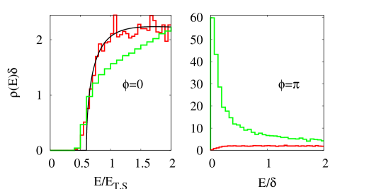
Figure 11: Density of states of closed Andreev billiards, for $\phi=0$ (left panel) and $\phi=\pi$ (right panel), in the universal regime with $M=2048$, $N_{\rm S}=25$ and $K=148$ (red curves, $\tau_{\rm E}/\tau_{\rm D,S}=0$, data averaged over 2500 samples) and in the semiclassical regime with $M=8192$, $N_{\rm S}=800$ and $K=10$ (green curves, $\tau_{\rm E}/\tau_{\rm D,S}=0.55$, 500 samples). The black curves indicate the universal predictions Mel96 ; Zir97 . Note the different horizontal and vertical scales.

\psfrag{G(phi)}{$G(\phi)$}\psfrag{G(pi)}{$G(\pi)$}\psfrag{G(pi)/G(0)}{$\mbox{ $G(\pi)/G(0)$}$}\psfrag{phi/2pi}{$\phi/2\pi$}\psfrag{kfl}{$M$}\includegraphics[width=241.84842pt]{fig12.eps}

Figure 12: Conductance through a chaotic Andreev interferometer vs. the phase difference $\phi$ between the two superconductors. Circles are numerical results obtained from the Andreev kicked rotator with $\Gamma_{\rm N}=0.01$, $M=8192$, $M/N_{\rm N}=20$, $M/N_{\rm S}=10$ and $K=10$. The green curve is the analytical prediction obtained by summing the semiclassical resonant contributions with the universal prediction. The red curve gives the universal prediction obtained from circuit theory. Left inset: Numerical data for the same classical parameters $M/N_{\rm N}=20$, $M/N_{\rm S}=10$ and $K=10$ as in the main plot, for $M=128$ (blue curve), 512 (green curve), 2048 (red curve), to 8192 (black curve). Note the change in peak-to-valley ratio. Right inset: peak-to-valley ratio $G(\pi)/G(0)$ (black squares) and peak conductance $G(\pi)$ (red circles) as a function of $M$ controlling the quantum-to-classical crossover, for the same classical configuration as in the main plot. Data are averaged over 150–1000 sample realizations.

In Fig. 12, we next show a conductance resonance curve in the semiclassical regime. We obtain very good agreement between the numerical data (circles) and the analytical prediction (green solid line) with $\tau_{\rm E}/\tau_{\rm D,S}\simeq 0.79$. Without the semiclassical contribution, the universal prediction of Eqs. (III.1–16) in the full range $\phi\in[0,2\pi]$ is given by the red line. While the latter fits the resonance curve far away from resonance, the agreement breaks down close to $\phi=\pi$, where universal contributions give a prediction $G(\pi)=2G_{0}$, too small by an order of magnitude. The left inset in Fig. 12 illustrates the increase of the peak height and narrowness as the semiclassical parameter $M$ increases. The four sets of data in this inset correspond to a fixed set of classical parameters, with the electronic wavelength decreasing by factors of four from one curve to the next, starting from the bottommost (blue) curve. The conductance increases at each step because the number of conduction channels scales linearly with $M$. In absence of semiclassical contributions, these four curves would exhibit the same peak-to-valley ratio, but here they do not. This is quantified in the right inset to Fig. 12, where we show both the peak height and the peak-to-valley ratio corresponding to the same classical configuration as in the main plot, while varying $M$.

We can connect the data in Figs. 11 and 12, since they correspond to the same closed Andreev billiard. The broadening of levels due to the external normal leads is $\delta E\simeq\Gamma_{\rm N}N_{\rm N}\delta/2\pi$. For the resonance in Fig. 12, this gives $\delta E=2\delta/\pi$. From the green curve in Fig. 11, we estimate that this value of $\delta E$ covers about 20 to 30 levels around the Fermi energy. Those states condense on classical orbits bouncing on average $M/2N_{\rm S}=5$ times at the billiard’s boundary. At each bounce, they have a probability $\simeq 1-2N_{\rm N}/(M-2N_{\rm S})$ not to touch a normal lead. Therefore, since $[1-2N_{\rm N}/(M-2N_{\rm S})]^{5}\approx 1/2$ for the data in Fig. 12 with $N_{\rm N}=400$ channels, we estimate that about half of these 20–30 states couple to the leads. One thus expects a resonant contribution to the conductance $\sim 10-15G_{0}$, which agrees quite well with the numerical value of $G(\pi)\simeq 16G_{0}$ for the data of Fig. 12, with a universal contribution of $2G_{0}$.

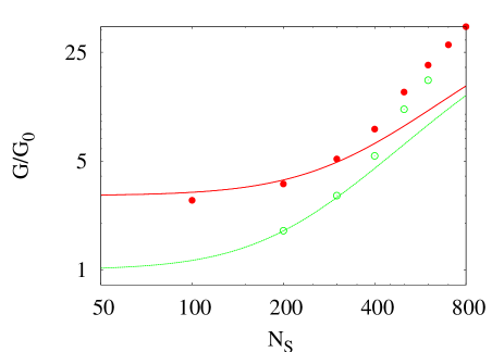
Figure 13: The conductance of the Andreev kicked rotator as a function of $N_{\rm S}$ for $K=10$, $M=4096$, $\Gamma_{\rm S}=1$, $\phi=\pi$, $N_{\rm N}=200$ and $\Gamma_{\rm N}=0.03$ (closed circles), $\Gamma_{\rm N}=0.01$ (open circles). Every data point is an average over at least $80$ realizations. The lines represent a sum of the semiclassical prediction Eq. (III.2) in the tunneling limit and the RMT result of Eq. (20) for $\Gamma_{\rm N}=0.03$ (solid red line) and $\Gamma_{\rm N}=0.01$ (dashed green line).

In Fig. 13 we show the conductance as a function of the number of channels in each superconducting lead $N_{\rm S}$, for two different values of $\Gamma_{\rm N}$. We see that the conductance depends strongly on $N_{\rm S}$, in contrast to the RMT prediction $G=G_{0}\Gamma_{\rm N}N_{\rm N}/2$ which is independent of it. In the parameter range of the figures, the contribution of Eq. (III.2) can be neglected and the contribution of Eq.  (III.2) dominates. For $\phi=\pi$ and $\Gamma_{\rm N}\rightarrow 0$, it can be simplified to $T_{LL}^{he}=(\pi N_{\rm N}/16)\left(1-(1+\tau_{\rm E}/\tau_{\rm D,S})\exp[-\tau_{\rm E}/\tau_{\rm D,S}]\right)$. This contribution depends strongly on $N_{\rm S}$ since both the Ehrenfest time and the time $\tau_{\rm D,S}$ between Andreev reflections depend on $N_{\rm S}$. It is therefore the relative measure of trajectories of class ${\rm I}$ which causes the order-of-magnitude increase of conductance with $N_{\rm S}$ observed in Fig. 13. The solid lines give the theoretical prediction obtained by summing the semiclassical resonant contribution, Eqs. (III.2) and (III.2), and the universal contribution obtained from Eqs. (III.1) and (16). There is good agreement between the numerical data and the theory, as long as the superconduting dwell time is long enough. For $N_{\rm S}>400$, $\tau_{\rm D,S}<5$, and we suspect that short processes across the billiard increase the conductance well above the analytical prediction.

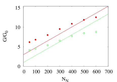
Figure 14: The conductance of the Andreev kicked rotator as a function of $N_{\rm N}$ for $K=10$, $M=4096$, $N_{\rm S}=400$, $\Gamma_{\rm S}=1$, $\phi=\pi$ and $\Gamma_{\rm N}=6/N_{\rm N}$ (closed circles), $\Gamma_{\rm N}=2/N_{\rm N}$ (open circles). Every data point is an average over at least $80$ realizations. The lines represent a sum of the semiclassical prediction Eq. (III.2) in the tunneling limit and the universal RMT result of Eq. (20) or $\Gamma_{\rm N}=6/N_{\rm N}$ (solid red line) and $\Gamma_{\rm N}=2/N_{\rm N}$ (dashed green line).

Finally, we show on Fig. 14 the conductance as a function of $N_{\rm N}$. The product $\Gamma_{\rm N}N_{\rm N}$ is kept constant, so that any observed $N_{\rm N}$ dependence arises from nonuniversal effects. Even though we always have moderate Ehrenfest times $\tau_{\rm E}<\tau_{\rm D,S}$, the numerical results are very different from the constant conductance predicted in the universal regime. The semiclassical contributions dominate and we see an increase of $G$ with $N_{\rm N}$. Here, $\tau_{\rm E}/\tau_{\rm D,S}\simeq 0.6$ is constant, and the increase of the conductance is predicted to be linear, see Eqs. (III.2) and (III.2). There is reasonable agreement between theory and numerical data, with significant deviations in the regime of small $N_{\rm N}$, where we leave the tunneling regime.

We conclude that our numerical data fully confirm our analytical results.

V Conclusion

We have presented analytical and numerical investigations of spectroscopy and transport in quantum chaotic Andreev billiards coupled to two superconductors. We identified two regimes with very different behaviors. In the universal regime, the presence of the superconductor opens up a gap in the density of states of the Andreev billiard at the Fermi level, which reduces the conductance through the system once it is attached to two external normal leads with tunnel contacts. This gap closes when the phase difference between the two superconductors is $\phi=\pi$, and in the tunneling limit, the normal conductance that the system would have in the absence of superconductivity is recovered. As the Fermi wavelength is reduced, $\lambda_{\rm F}/W_{\rm S},\;\lambda_{\rm F}/L_{\rm c}\ll 1$, one enters a new, semiclassical regime, where the situation is only marginally different unless the phase difference between the two superconductors is close to $\pi$. When this is the case, we found an order-of-magnitude enhancement of the tunneling conductance, and identified the mechanism behind this enhancement as resonant tunneling through a macroscopic number of quasi-degenerate levels at the Fermi energy of the corresponding closed Andreev billiard.

Our calculation focused on the zero-temperature limit of transport, and we finally comment on the effect of a finite temperature. From Fig. 10, we concluded that, in the universal regime, the shape of the conductance oscillations do not differ from those presented in Fig. 8, as long as the temperature lies below the superconducting Thouless energy, $E_{\rm T,S}=\Gamma_{\rm S}N_{\rm S}\delta/2\pi$. The semiclassical contribution to the conductance near $\phi=\pi$ is however much more sensitive to changes in temperatures than the universal one. Finite excitation energies indeed lead to an additional action phase accumulated along transport orbits. The expressions in Eqs. (36) and (III.2) are now combined into the following expression

$$\frac{1}{\tau_{\rm D,S}^{2}}\sum_{p,p^{\prime}=0}^{\infty}(1-\Gamma_{\rm n})^{a(p+p^{\prime})+b}\;\Gamma_{\rm s}^{p+p^{\prime}+c}\;e^{i(p-p^{\prime})(\phi-\pi)}\;\;\;\;\;\;\;\;$$ (59)

$$\times\int_{0}^{\tau_{\rm E}}{\rm d}t_{s1}\int_{0}^{\tau_{\rm E}-t_{s1}}{\rm d}t_{s3}\;e^{-[t_{s1}+t_{s3}][\tau_{\rm D,S}^{-1}+iE(p-p^{\prime})/\hbar]}.$$

The accumulation of an $E$-dependent action phase results in a cut-off for the summation over $p$ and $p^{\prime}$, effectively suppressing contribution with $p-p^{\prime}\gtrsim p_{\rm max}^{(-)}\equiv(\hbar/E\,\tau_{\rm D,S})^{2}$. One ends up with a prefactor $1-(1-\Gamma_{\rm N})^{p_{\rm max}^{(-)}}$ multiplying Eqs. (III.2) and (III.2), which suppresses the semiclassical contribution already for temperatures significantly smaller than $E_{\rm T,S}$. At finite temperature, the resonant conductance enhancement discussed above will thus be maximal for an intermediate value of $\Gamma_{\rm N}$ optimizing macroscopic resonant tunneling while minimizing thermal averaging.

References

• (1) A. F. Andreev, Zh. Eksp. Teor. Fiz. 46, 1823 (1964) [Sov. Phys. JETP 19 1228 (1964)].
• (2) Y. Imry, Introduction to Mesoscopic Physics (Oxford University, Oxford, 2002); B.J. van Wees and H. Takayanagi, in Mesoscopic Electron Transport, L.L. Sohn, L.P. Kouwenhoven and G. Schön Eds., NATO ASI Series E345 (Kluwer, Dordrecht, 1997).
• (3) I. Kosztin, D. L. Maslov, and P. M. Goldbart, Phys. Rev. Lett. 75, 1735 (1995).
• (4) J. A. Melsen, P. W. Brouwer, K. M. Frahm, and C. W. J. Beenakker, Europhys. Lett. 35, 7 (1996).
• (5) H. Schomerus and C. W. J. Beenakker, Phys. Rev. Lett. 82, 2951 (1999).
• (6) O. Bohigas, M. J. Giannoni, and C. Schmit. Phys. Rev. Lett. 52, 1 (1984); S. Müller, S. Heusler, P. Braun P, F. Haake, and A. Altland, Phys. Rev. Lett. 93, 014103 (2004).
• (7) A. Lodder and Yu. V. Nazarov, Phys. Rev. B 58, 5783 (1998).
• (8) H. Schomerus and Ph. Jacquod, J. Phys. A. 38, 10663 (2005).
• (9) M. G. Vavilov and A. I. Larkin, Phys. Rev. B 67, 115335 (2003).
• (10) İ. Adagideli and C. W. J. Beenakker, Phys. Rev. Lett. 89, 237002 (2002).
• (11) P. G. Silvestrov, M. C. Goorden, and C. W. J. Beenakker, Phys. Rev. Lett. 90, 116801 (2003).
• (12) Ph. Jacquod, H. Schomerus, and C. W. J. Beenakker, Phys. Rev. Lett. 90, 207004 (2003).
• (13) M. C. Goorden, Ph. Jacquod, and C. W. J. Beenakker, Phys. Rev. B 68, 220501(R) (2003).
• (14) A. Kormányos, Z. Kaufmann, C.J. Lambert, and J. Cserti, Phys. Rev. B 70, 052512 (2004).
• (15) M. C. Goorden, Ph. Jacquod, and C. W. J. Beenakker, Phys. Rev. B 72, 064526 (2005).
• (16) P.G. Silvestrov, Phys. Rev. Lett. 97, 067004 (2006).
• (17) J. A. Melsen, P. W. Brouwer, K. M. Frahm, and C. W. J. Beenakker, Physics Scripta T69, 223 (1997).
• (18) F. Zhou, P. Charlat, B. Spivak, and B. Pannetier, J. Low Temp. Phys. 110, 841 (1998).
• (19) D. Taras-Semchuk and A. Altland, Phys. Rev. B 64, 014512 (2001).
• (20) C. W. J. Beenakker, Rev. Mod. Phys. 69, 731 (1997).
• (21) A. Kadigrobov, A. Zagoskin, R.I. Shekhter, and M. Jonson, Phys. Rev. B 52, R8662 (1995). This article makes the unphysical assumption that the interferometer does not mix transport modes and therefore acts as $N$ identical one-dimensional interferometers in parallel.
• (22) H.A. Blom, A. Kadigrobov, A.M. Zagoskin, R.I. Shekhter, and M. Jonson, Phys. Rev. B 57, 9995 (1998). In this article, the chaoticity of the cavity is related to the strength of the tunnel barriers between the leads and the cavity in such a way that, in the tunneling limit, $\Gamma_{\rm N}\ll 1$, the cavity becomes regular.
• (23) B.Z. Spivak and D.E. Khmel’nitskii, JETP Lett. 35, 412 (1982). This work lies somehow outside our present focus, as it considers temperatures larger than $E_{\rm T,S}$.
• (24) A.V. Zaitsev, Phys. Lett. A 194, 315 (1994).
• (25) C.W.J. Beenakker, J.A. Melsen, and P.W. Brouwer, Phys. Rev. B 51, 13883 (1995).
• (26) A. Kadigrobov, L.Y. Gorelik, R.I. Shekhter, and M. Jonson, Superlattices and Microstructures 25, 961 (1999).
• (27) Y. V. Nazarov, Phys. Rev. Lett. 73, 1420 (1994).
• (28) N. Argaman, Europhys. Lett. 38, 231 (1997).
• (29) Ph. Jacquod and R. S. Whitney, Phys. Rev. B 73, 195115 (2006).
• (30) K. Richter and M. Sieber, Phys. Rev. Lett. 89, 206801 (2002); S. Heusler, S. Müller, P. Braun, and F. Haake, Phys. Rev. Lett. 96, 066804 (2006).
• (31) İ. Adagideli, Phys. Rev. B 68, 233308 (2003).
• (32) P. W. Brouwer and S. Rahav, Phys. Rev. B 74, 075322 (2006).
• (33) R.S. Whitney, Phys. Rev. B 75, 235404 (2007).
• (34) K.M. Frahm, P.W. Brouwer, J.A. Melsen, and C.W.J. Beenakker, Phys. Rev. Lett. 76, 2981 (1996).
• (35) A. Altland and M. R. Zirnbauer, Phys. Rev. B 55, 1142 (1997).
• (36) W. Ihra, M. Leadbeater, J.L. Vega, and K. Richter, Eur. Phys. J. B 21, 425 (2001); O. Zaitsev, J. Phys. A 39, L467 (2006).
• (37) S. Iida, H.A. Weidenmüller, and J.A. Zuk, Phys. Rev. Lett. 64, 583 (1990).
• (38) C.J. Lambert, J. Phys. Cond. Mat. 5, 707 (1993); N. R. Claughton and C. J. Lambert, Phys. Rev. B 53, 6605 (1996).
• (39) L. Couchman, E. Ott, and T.M. Antonsen, Phys. Rev. A 46, 6193 (1992).
• (40) The segments $\gamma_{si}$, $i=1,2,3$ in Fig.5 might include many intermediate bounces at a tunnel barrier. All possible number of reflections are effectively resummed; see Ref. Whi07 for more details.
• (41) F. Haake, Quantum Signatures of Chaos, 2nd Ed. Springer, Berlin (2001).
• (42) R. Ketzmerick, K. Kruse, and T. Geisel, Physics D 131, 247 (1999).
• (43) Y. V. Fyodorov and H.-J. Sommers, JETP Lett. 72, 422 (2000).
• (44) J. Tworzydło, A. Tajic and C. W. J. Beenakker, Phys. Rev. B 68, 115313 (2003).