Exact and Approximate Expressions for the Probability of Undetected Error of Varshamov-Tenengol’ts Codes

Abstract

Computation of the undetected error probability for error correcting codes over the Z-channel is an important issue, explored only in part in previous literature. In this paper we consider the case of Varshamov-Tenengol’ts codes, by presenting some analytical, numerical, and heuristic methods for unveiling this additional feature. Possible comparisons with Hamming codes are also shown and discussed.

I Introduction

The Z-channel is a memoryless binary channel. For this channel, a 1 can be changed to a 0 with some probability $p$ (called the channel error probability), but a 0 is not changed. This channel is a useful model for a number of applications, like semiconductor memories, some kinds of optical systems, and other practical environments (examples can be found in [1, Chapter 7] and [2]). In [3], it was demonstrated that the Z-channel is the only binary-input binary-output channel that is never dropped in optimal probability loading for parallel binary channels with a total probability constraint. For a survey of classical results on codes for the Z-channel, see [4].

Several constructions can be adopted for designing codes over the Z-channel with given length and error correction capability, and bounds on their size can be derived, based on each specific construction [5]. For single error correcting codes, that are of interest in this paper, further bounds can be found in [6].

We consider a well known class of single error correcting codes for the Z-channel, that is the class of Varshamov-Tenengol’ts (VT) codes [7]. We describe these codes and some of their properties. Let $F_{2}=\{0,1\}$ denote the binary field, and let $Z_{n+1}$ be the additive group of integers modulo $n+1$. For each $g\in Z_{n+1}$, the VT code $V_{g}$ of length $n$ is the set of vectors ${\mathbf{x}}=(x_{1},x_{2},\ldots,x_{n})\in F_{2}^{n}$ such that

$$\sum_{m=1}^{n}mx_{m}\equiv g\pmod{n+1}.$$ (1)

We can observe that the all-zero codeword, noted by ${\mathbf{0}}$, always belongs to $V_{0}$, while the all-one codeword, noted by ${\mathbf{1}}$, belongs to $V_{g}$ with $g=\lfloor\frac{n+1}{2}\rfloor$, where $\lfloor x\rfloor$ is the largest integer $m$ such that $m\leq x$.

Construction (1) can be generalized using other abelian groups of size $n+1$. The corresponding codes are known as Constantin-Rao (CR) codes. In this paper we only consider VT codes, but most of our results can easily be generalized to CR codes.

The Hamming weight of ${\mathbf{x}}=(x_{1},x_{2},\ldots,x_{n})\in F_{2}^{n}$ is $w({\mathbf{x}})=\#\{m\mid x_{m}=1\}$.

We use $\#V_{g}$ to denote the size of $V_{g}$ and $A_{0}^{(g)},A_{1}^{(g)},\ldots,A_{n}^{(g)}$ to denote its weight distribution, that is, $A_{i}^{(g)}$ is the number of codewords in $V_{g}$ of Hamming weight $i$. Exact formulas for the size and weight distribution of $V_{g}$ were first determined by Mazur [8]. They were later generalized to the larger class of CR codes [9]. In particular, it is known that $\#V_{0}\geq\#V_{g}$ for all $g>0$. The codes have all size approximately $2^{n}/(n+1)$. More precisely,

$$\frac{2^{n}}{n+1}\leq\#V_{0}\leq\frac{2^{n}}{n+1}\Bigl{\{}1+\frac{n}{2^{2(n+2)/3}}\Bigr{\}}.$$

Further

$$A_{j}^{(0)}=\frac{1}{n+1}\sum_{d|(n+1)}(-1)^{j+\lfloor j/d\rfloor}{\frac{n+1}{d}-1\choose\lfloor j/d\rfloor}\varphi(d)$$ (2)

where $\varphi(d)$ is the Euler’s totient function.

Taking only the main term of (2) we get the approximation

$$A_{j}^{(0)}\approx\frac{1}{n+1}{n\choose j}.$$ (3)

We let ${\mathbf{y}}=(y_{1},y_{2},\ldots,y_{n})\leq{\mathbf{x}}=(x_{1},x_{2},\ldots,x_{n})$ denote that $y_{m}\leq x_{m}$ for $1\leq m\leq n$.

When ${\mathbf{x}}$ is sent, then only vectors ${\mathbf{y}}\leq{\mathbf{x}}$ can be received, and the probability for this to happen is

$$p^{w({\mathbf{x}})-w({\mathbf{y}})}(1-p)^{w({\mathbf{y}})}=p^{w({\mathbf{e}})}(1-p)^{w({\mathbf{x}})-w({\mathbf{e}})}$$

where ${\mathbf{e}}={\mathbf{x}}-{\mathbf{y}}$ is the error vector.

A systematic version of VT codes was studied in [10].

Many properties of these codes, either in systematic or non-systematic form, were explored in the past but, at the best of our knowledge, no attention has been paid up to now to their error detection properties.

In this paper, we provide a first contribution for filling such gap. Our analysis is mainly focused on the VT code $V_{0}$. However, we will also give some results for codes $V_{g}$ with $g\neq 0$. Some comparisons will be also developed with the well known family of Hamming codes, finding important performance similarities, both when these codes are applied over the Z-channel and even over the symmetric channel.

The paper is organized as follows. In Section II we introduce the probability of undetected error, $P_{\mathrm{u}e}$. In Section III we give an exact formula for $P_{\mathrm{u}e}$, that can be explicitly computed for small lengths $n$ (up to approximately 25). Next, in Section IV we study good lower bounds that can be explicitly computed up to almost twice this length (depending on how tight we require the bounds to be). In Section V we look at the class of Hamming codes, for the sake of comparison, and their application is considered for both the symmetric channel and the asymmetric one; a first performance comparison with VT codes is done, for small lengths. In Section VI we use some heuristic arguments to give a very good approximation that can easily be computed even for large lengths. In Section VII we use Monte Carlo methods to obtain other good approximations for long code lengths; this permits us also to make other comparisons with Hamming codes of the same length. Finally, in Section VIII, some remarks on future research conclude the paper.

II The probability of undetected error

For a description of properties of the probability of undetected error, see [11]. In general, an undetected error occurs when, in presence of one or more errors, the received sequence coincides with a codeword different from the transmitted one. In this case the decoder accepts the received sequence, and information reconstruction is certainly wrong. By the VT code construction, single errors are always detected, so that undetected errors can appear only when the number of errors is greater than one.

We note that, if ${\mathbf{x}}\in V_{g}$ is sent and ${\mathbf{y}}$ is received, then ${\mathbf{y}}\in V_{g}$ if and only if ${\mathbf{e}}={\mathbf{x}}-{\mathbf{y}}\in V_{0}$. This can be proved by observing that:

$$\sum_{m=1}^{n}me_{m}=\sum_{m=1}^{n}mx_{m}-\sum_{m=1}^{n}my_{m}\equiv g-g=0\pmod{n+1}.$$

Hence, the undetectable errors are exactly the non-zero vectors in $V_{0}$. For $j\geq 0$, let

$${\cal{E}}_{j}({\mathbf{x}})=\{{\mathbf{e}}\in V_{0}\mid w({\mathbf{e}})=j,\ {\mathbf{e}}\leq{\mathbf{x}}\}.$$

For $j>0$, this is the set of undetectable errors of weight $j$ when ${\mathbf{x}}$ is transmitted. We note that ${\cal{E}}_{0}({\mathbf{x}})=\{{\mathbf{0}}\}$ (and ${\mathbf{0}}$ is not an error vector). Let $\varepsilon_{j}({\mathbf{x}})$ be the size of ${\cal{E}}_{j}({\mathbf{x}})$. Note that since $V_{0}$ does not contain any vector of weight one, we have $\varepsilon_{1}({\mathbf{x}})=0$ for all ${\mathbf{x}}$. We also have $\varepsilon_{0}({\mathbf{x}})=1$ for all ${\mathbf{x}}$.

The (average) probability of undetected error is given by

$$P_{\mathrm{u}e}(V_{g},p)=\frac{1}{\#V_{g}}\sum_{{\mathbf{x}}\in V_{g}}\sum_{j=2}^{w({\mathbf{x}})}\varepsilon_{j}({\mathbf{x}})p^{j}(1-p)^{w({\mathbf{x}})-j}.$$ (4)

In deriving (4), the codewords are assumed equally probable. If we define

$$A_{i,j}^{(g)}=\sum_{{{\mathbf{x}}\in V_{g}\atop w({\mathbf{x}})=i}}\varepsilon_{j}({\mathbf{x}}),$$

(4) can be rewritten

$$P_{\mathrm{u}e}(V_{g},p)=\frac{1}{\#V_{g}}\sum_{i=2}^{n}\sum_{j=2}^{i}A_{i,j}^{(g)}p^{j}(1-p)^{i-j}.$$ (5)

III Exact evaluation of the undetected error probability

Conceptually, the simplest way to compute the undetected error probability consists in direct calculation of (4) by first determining the sets ${\cal{E}}_{j}({\mathbf{x}})$. Since both $V_{g}$ and $V_{0}$ have size on the order of $2^{n}/(n+1)$, the complexity is on the order of $2^{2n}/(n+1)^{2}$.

III-A $P_{\mathrm{u}e}(V_{0},p)$

We observe that if ${\mathbf{x}}=(x_{1},x_{2},\ldots,x_{n})\in V_{0}$, then the reversed vector

$${\mathbf{x}}^{\rho}=(x_{n},x_{n-1},\ldots,x_{1})\in V_{0},$$

too, since

$$\sum_{m=1}^{n}mx_{n+1-m} = \sum_{m=1}^{n}(n+1-m)x_{m}$$

$$= w({\mathbf{x}})(n+1)-\sum_{m=1}^{n}mx_{m}$$

$$\equiv 0-0=0\pmod{n+1}.$$

This simplifies the calculations and reduces the complexity by some factor, but the order of magnitude of the complexity is still the same. We will elaborate on this symmetry in the next section.

Another observation is that if $w({\mathbf{x}})=i$ and ${\mathbf{e}}\in{\cal{E}}_{j}({\mathbf{x}})$, with $j\leq i$, then ${\mathbf{y}}\in{\cal{E}}_{i-j}({\mathbf{x}})$. Hence,

$$A_{i,j}^{(0)}=A_{i,i-j}^{(0)}\mbox{ for }0\leq j\leq i\leq n.$$ (6)

This again halves the complexity for $g=0$. For completeness, we also observe that

$$A_{i,i}^{(0)}=A_{i}^{(0)}\mbox{ for }0\leq i\leq n,$$ (7)

$$A_{i,1}^{(0)}=0\mbox{ for }1\leq i\leq n.$$ (8)

For even $n$, further symmetry properties can be found.

For any vector $\mathbf{x}=(x_{1},x_{2},\ldots,x_{n})$, the complementary vector $\bar{\mathbf{x}}$ is defined by

$$\bar{\mathbf{x}}=(1-x_{1},1-x_{2},\ldots,1-x_{n}),$$

that is, $\bar{x}_{m}=1$ if $x_{m}=0$ and $\bar{x}_{m}=0$ if $x_{m}=1$. Clearly,

$$w(\bar{\mathbf{x}})=n-w(\mathbf{x})$$

and

$$\sum_{m=1}^{n}m\bar{x}_{m}=\frac{n^{2}(n+1)}{2}-\sum_{m=1}^{n}mx_{m}.$$

This implies that if $n$ is even and ${\mathbf{x}}\in V_{0}$, then $\bar{\mathbf{x}}\in V_{0}$. Next, we observe that if ${\mathbf{y}}\leq{\mathbf{x}}$, then $\bar{\mathbf{x}}\leq\bar{\mathbf{y}}$. In particular, this implies the relation

$$A_{i,j}^{(0)}=A_{n-j,n-i}^{(0)}\mbox{ for }0\leq j\leq i\leq n.$$ (9)

We note that this relation is not valid for odd $n$.

Relations (6) and (9) can be combined. For example, (9) implies that $A_{i,i-j}^{(0)}=A_{n-i+j,n-i}^{(0)}$. Next, (6) implies that $A_{n-i+j,n-i}^{(0)}=A_{n-i+j,j}^{(0)}$, etc. Repeated use of (6) and (9) gives the following result:

if $n$ is even and $0\leq j\leq i\leq n$, then

$$A_{i,j}^{(0)} = A_{i,i-j}^{(0)}=A_{n-i+j,n-i}^{(0)}=A_{n-i+j,j}^{(0)}$$ (10)

$$= A_{n-j,i-j}^{(0)}=A_{n-j,n-i}^{(0)}.$$

Putting $i=j$ in (10) and combining with (7) we also get

$$A_{n,j}^{(0)}=A_{j}^{(0)}=A_{n-j}^{(0)}.$$ (11)

Using these relations, for even $n$, the complexity of the exact calculus for $g=0$ is further reduced. For odd $n$, the same relationships are not valid. Moreover, it should be noted that, for odd $n$ we have $A_{n}^{(0)}=A_{n,j}^{(0)}=0$.

We have developed a numerical program, in the C++ language, that constructs all the sets ${\cal{E}}_{j}({\mathbf{x}})$ for ${\mathbf{x}}\in V_{0}$ (exploiting the symmetry properties discussed above) and, based on this, computes the numbers $A_{i,j}^{(0)}$. The values of $P_{{\rm ue}}(V_{0},p)$ as a function of $p$ computed this way are exact.

Examples of the results obtained are shown in Fig. 1, for $n=10,15,20,25$. For small values of $p$, up to about 0.2, small values of $n$ give lower probability of undetected error, whilst for larger values of $p$ the behavior of codes with larger $n$ is better.

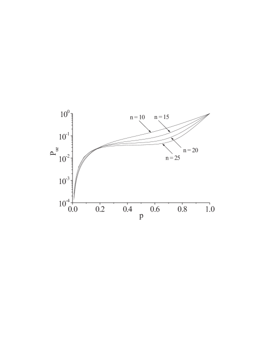
Figure 1: $P_{{\rm ue}}(V_{0},p)$ vs. $p$ for some values of $n$.

For $p=1$ all codewords are changed to ${\mathbf{0}}$, and this implies:

$$P_{{\rm ue}}(V_{0},1)=\frac{\#V_{0}-1}{\#V_{0}},$$

that is slightly different from 1 because of the presence of the all-zero codeword (that is always received correctly).

III-B $P_{\mathrm{u}e}(V_{g},p)$ for $g\neq 0$

For $g\neq 0$, $V_{g}$ does not include the all-zero vector. As a consequence, $P_{\mathrm{u}e}(V_{g},1)=0$ and the curve of $P_{{\rm ue}}$ has at least one maximum for $p$ between 0 and 1. As for $V_{0}$, we have developed a computer program that permits us to calculate exactly the undetected error probability of these codes, as a function of $p$, for not too high values of $n$ (in such a way as to have acceptable processing times).

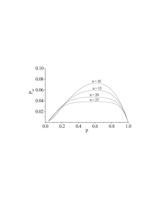
Figure 2: $P_{{\rm ue}}(V_{1},p)$ vs. $p$ for some values of $n$.

In Fig. 2, curves of $P_{\mathrm{u}e}(V_{1},p)$ are plotted, for some values of $n$. For better readability, we have used a linear scale instead of the logarithmic one used in Fig. 1.

These curves have been obtained for $g=1$, but they remain practically the same for codes $V_{g}$, with $g>1$.

A main reason why $P_{\mathrm{u}e}(V_{0},p)$ and $P_{\mathrm{u}e}(V_{1},p)$ behave differently for large $p$ is that $V_{0}$ contains the all-zero vector. If we remove the all-zero codeword, that is consider

$$V_{0}^{\prime}=V_{0}\setminus\{{\mathbf{0}}\}$$

instead, we get:

$$P_{{\rm ue}}(V_{0}^{\prime},p)=P_{{\rm ue}}(V_{0},p)-\frac{\sum_{j=1}^{n}A_{j}^{(0)}p^{j}}{\#V_{0}}$$

and code $V_{0}^{\prime}$ has no undetectable errors for $p=1$. It turns out that $P_{\mathrm{u}e}(V_{0}^{\prime},p)$ and $P_{\mathrm{u}e}(V_{1},p)$ are almost the same for $p<0.5$ but they differ somewhat in the region $[0.5,1]$. We illustrate this behavior for $n=20$, in Fig. 3.

Figure 3: Comparison of $P_{{\rm ue}}(V_{0}^{\prime},p)$ and $P_{{\rm ue}}(V_{1},p)$ for $n=20$.

IV Lower bounds on $P_{{\rm ue}}$

Clearly, if we omit or reduce some of the terms in (5), we get a lower bound on $P_{\mathrm{u}e}(V_{g},p)$. For example, for a fixed integer $m\geq 2$, then

$$P_{\mathrm{u}e}(V_{g},p)\geq\frac{1}{\#V_{g}}\sum_{i=2}^{n}\sum_{j=2}^{\min(m,i)}A_{i,j}^{(g)}p^{j}(1-p)^{i-j}.$$

The number of errors of weight $j$ is upper bounded by $A_{j}^{(0)}\approx\frac{1}{n+1}{n\choose j}$. Hence, the complexity of calculating the coefficients $A_{i,j}^{(g)}$ for $j\leq m$ is on the order of

$$\frac{2^{n}{n\choose m}}{(n+1)^{2}}.$$

For small values of $m$, this is of course much lower than the computations needed to determine all the $A_{i,j}^{(g)}$ which we estimated to be on the order of $2^{2n}/(n+1)^{2}$.

Next, we describe in detail how to calculate $A_{i,j}^{(0)}$ for $j=2$, $j=3$ and $j=4$. First, we remind the reader that the support $\chi({\mathbf{e}})$ of a vector ${\mathbf{e}}$ is the set of positions where the vector has ones, that is

$$\chi({\mathbf{e}})=\{r\mid e_{r}=1\}.$$

• Calculus of $A_{i,2}^{(0)}$

If ${\mathbf{e}}\in V_{0}^{\prime}$ has weight 2, and

$$\chi({\mathbf{e}})=\{r,s\},$$

where $1\leq r<s\leq n$, then, by the definition of the code, we must have

$$r+s=n+1.$$

Hence $s=n+1-r\geq r+1$ and so $r\leq n/2$. Therefore, ${\mathbf{e}}\in{\cal{E}}_{2}({\mathbf{x}})$ if and only if $x_{r}=x_{n+1-r}=1$. Hence

$$\varepsilon_{2}({\mathbf{x}})=\sum_{r=1}^{\lfloor n/2\rfloor}x_{r}x_{n+1-r},$$

and

$$A_{i,2}^{(0)}=\sum_{{{\mathbf{x}}\in V_{0}^{\prime}\atop w({\mathbf{x}})=i}}\sum_{r=1}^{\lfloor n/2\rfloor}x_{r}x_{n+1-r}.$$

• Calculus of $A_{i,3}^{(0)}$

If ${\mathbf{e}}\in V_{0}^{\prime}$ has weight 3, and

$$\chi({\mathbf{e}})=\{r,s,t\}$$

where $1\leq r<s<t\leq n$, then we must have

$$r+s+t=n+1\mbox{ or }r+s+t=2(n+1).$$

We observe that if ${\mathbf{e}}\leq{\mathbf{x}}$ then, clearly, ${\mathbf{e}}^{\rho}\leq{\mathbf{x}}^{\rho}$ (the reversed vectors). Further,

$$\chi({\mathbf{e}}^{\rho})=\{n+1-t,n+1-s,n+1-r\}$$

and

$$(n+1-t)+(n+1-s)+(n+1-r)=3(n+1)-(r+s+t).$$

Hence, for each error with support that sums to $n+1$, there is another (reversed) error with support that sums to $2(n+1)$. Therefore, it is sufficient to consider the first kind, this way deriving a contribution that is exactly half of $A_{i,3}^{(0)}$. If $r+s+t=n+1$, then we have

$$n+1=r+s+t\geq r+(r+1)+(r+2)$$

and so $r\leq(n-2)/3$. Further,

$$n+1-r=s+t\geq s+(s+1)$$

and so $s\leq(n-r)/2$. Hence, similarly to what we did for $j=2$, we get

$$A_{i,3}^{(0)}=2\sum_{{{\mathbf{x}}\in V_{0}^{\prime}\atop w({\mathbf{x}})=i}}\sum_{r=1}^{\lfloor(n-2)/3\rfloor}\sum_{s=r+1}^{\lfloor(n-r)/2\rfloor}x_{r}x_{s}x_{n+1-r-s}.$$

• Calculus of $A_{i,4}^{(0)}$

If ${\mathbf{e}}\in V_{0}^{\prime}$ has weight 4, and

$$\chi({\mathbf{e}})=\{r,s,t,u\}$$

where $1\leq r<s<t<u\leq n$, then one of the following conditions should be satisfied:

1. $r+s+t+u=n+1$,

2. $r+s+t+u=2(n+1)$,

3. $r+s+t+u=3(n+1)$.

However, we observe that when vector $\mathbf{e}$ satisfies condition i) then the reversed vector ${\mathbf{e}}^{\rho}$ satisfies condition iii) and vice versa. In fact:

$$(n+1-u)+(n+1-t)+(n+1-s)+(n+1-r)=$$

$$=4(n+1)-(r+s+t+u)=3(n+1).$$

Hence, for each error with support that sums to $n+1$, there is another (reversed) error with support that sums to $3(n+1)$. Therefore, it is sufficient to consider condition i) and then double the size so found for taking into account also condition iii). If $r+s+t+u=n+1$, we have

$$n+1=r+s+t+u\geq r+(r+1)+(r+2)+(r+3)=4r+6$$

and so $r\leq(n-5)/4$. On the other hand,

$$n+1-r=s+t+u\geq s+(s+1)+(s+2)=3s+3$$

and so $s\leq(n-2-r)/3$. Finally

$$n+1-r-s=t+u\geq t+(t+1)=2t+1$$

and so $t\leq(n-r-s)/2$.

Similarly, we can consider condition ii). It implies:

$$2n+2=r+s+t+u\geq 4r+6$$

and so $r\leq(2n-4)/4$. Further

$$2n+2-r=s+t+u\geq 3s+3$$

and so $s\leq(2n-1-r)/3$. Finally

$$2n+2-r-s=t+u\geq 2t+1$$

and so $t\leq(2n+1-r-s)/2$.

On the basis of such analysis, the expression of $A_{i,4}^{(0)}$ can be written as follows:

$$A_{i,4}^{(0)} = 2\sum_{{{\mathbf{x}}\in V_{0}^{\prime}\atop w({\mathbf{x}})=i}}\sum_{r=1}^{\lfloor(n-5)/4\rfloor}\sum_{s=r+1}^{\lfloor(n-2-r)/3\rfloor}$$

$$\quad\sum_{t=s+1}^{\lfloor(n-r-s)/2\rfloor}x_{r}x_{s}x_{t}x_{n+1-r-s-t}$$

$$+\sum_{{{\mathbf{x}}\in V_{0}^{\prime}\atop w({\mathbf{x}})=i}}\sum_{r=1}^{\lfloor(2n-4)/4\rfloor}\sum_{s=r+1}^{\lfloor(2n-1-r)/3\rfloor}$$

$$\quad\sum_{t=\max(s+1,n+2-r-s)}^{\lfloor(2n+1-r-s)/2\rfloor}x_{r}x_{s}x_{t}x_{2n+2-r-s-t}.$$

It should be noted that, in the inner sum of the second contribution (the one due to condition ii)), we have explicitly taken into account that $t$ cannot be smaller than $n+2-r-s$; this is because the following obvious condition must be satisfied

$$u=2(n+1)-(r+s+t)\leq n$$

that implies

$$n+2-r-s\leq t.$$

Additionally, the sums appearing in the expressions of $A_{i,j}^{(0)}$ are null when the upper extreme is smaller than the lower extreme. So, the first contribution in $A_{i,4}^{(0)}$ is not present for $n\leq 8$, and also the second contribution disappears (as obvious) for $n\leq 3$.

Though the procedure adopted to derive $A_{i,2}^{(0)}$, $A_{i,3}^{(0)}$ and $A_{i,4}^{(0)}$ is quite clear and, in principle, can be extended to the other values of $j$, it is easy to see that, formally, the analysis becomes more and more tedious for increasing $j$. Similarly, explicit formulas can be given for $A_{i,j}^{(g)}$ for $g\neq 0$, but they are usually somewhat more complicated. The formula for $j=2$ generalizes immediately to

$$A_{i,2}^{(g)}=\sum_{{{\mathbf{x}}\in V_{g}\atop w({\mathbf{x}})=i}}\sum_{r=1}^{\lfloor n/2\rfloor}x_{r}x_{n+1-r}.$$

However, for $j=3$ we used above the symmetry that only appears in $V_{0}$, and so the formula for $A_{i,3}^{(g)}$ will contain two sums in the expression. Similarly for $j\geq 4$.

For $V_{0}$ we have computed some lower bounds for $n=10,15,20$ and $25$ to see how good the bounds are, in comparison with the exact values. In the lower bound we have used $A_{i,2}$, $A_{i,3}$, and $A_{i,4}$ for $4\leq i\leq n$ computed by the formulas above, $A_{i,i-2}$, $A_{i,i-3}$, $A_{i,i-4}$ which have the same values by (6), and finally $A_{i,i}$ obtained from (7). The remaining terms have been set to zero. The lower bounds and the exact values are compared in Fig. 4.

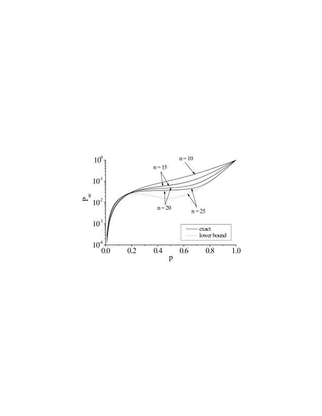
Figure 4: The lower bounds and the exact results for $P_{\mathrm{u}e}(V_{0},p)$ for lengths $n=10,15,20,25$.

From the figure we see that the lower bound is an excellent approximation of the true behavior for $n=10$ (the exact curve and the bound are superposed), that the approximation is very good for $n=15$, but that the difference between the exact curve and the estimated one becomes more and more evident for increasing $n$. Qualitatively, such a trend seems quite obvious and expected. In particular, the lower bound for $n=25$ exhibits an oscillation, in the central region, which is due to the terms neglected, whose effect is particularly important in the neighborhood of $p=0.5$. On the other hand, it is easy to verify that the approximation is very good, independently of $n$, for small values of the channel error probability $p$. Even the simple bound using only $A_{i,2}^{(0)}$ gives a good approximation for small $p$.

V Comparison with Hamming codes and relationship with the symmetric channel

Hamming codes are another well known class of single error correcting codes, widely used both in symmetric and asymmetric channels. In particular, they are known to be optimal error detecting codes for the the binary symmetric channel (BSC) [12].

The length of a binary Hamming code $H$ is $n=2^{r}-1$, where $r$ is the number of parity check bits, while the number of codewords (i.e., the size of the code) is $M=2^{k}$, with $k=2^{r}-1-r$. For a description of Hamming codes and their properties see, for example, [13].

The dual codes of Hamming codes are maximal length (or simplex) codes, which means that the generator matrix of a Hamming code can be used as the parity check matrix of a maximal length code, and vice versa.

The weight distribution of these codes is known:

$$A_{i}^{H}=\frac{{n\choose i}+n(-1)^{\lceil i/2\rceil}{(n-1)/2\choose\lfloor i/2\rfloor}}{n+1}.$$

Here $\lceil x\rceil$ denotes the smallest integer $m$ such that $m\geq x$.

When the code is applied over the BSC, this permits to find an explicit expression for the probability of undetected error [11, p. 44], namely:

$$P_{{\rm ue}}^{{\rm BSC}}(H,p)=\frac{1}{n+1}\left[1+n(1-2p)^{(n+1)/2}\right]-(1-p)^{n}.$$ (12)

In this expression, $p$ represents either the probability that a 1 is changed to a 0 or a 0 is changed to a 1.

However, as for VT codes, an explicit expression for $P_{{\rm ue}}(H,p)$ is not available for the case of the Z-channel. Similarly to what was done in Section III, we have developed a numerical program, in C++ language, that permits to evaluate, exhaustively, all transitions yielding undetected errors. The procedure is conceptually similar to that described in Section II, for VT codes, and an expression like (5) still holds, as an undetected error occurs if and only if the error vector belongs to $H$.

The curve of $P_{{\rm ue}}(H,p)$ can be compared, for a fixed $n$, with that of $P_{{\rm ue}}(V_{0},p)$. An example is shown in Fig. 5 for $n=15$; both codes have the same number of codewords, i.e., $\#V_{0}=M=2048$. The two curves are rather similar, but the performance of the Hamming code is slightly better. In Section VII we will do a comparison for a larger $n$. There we show that for $n=127$ both curves are dominated by a nearly flat region in the neighborhood of $p=0.5$. The extent of the nearly flat region becomes wider and wider for increasing $n$. The rationale for the existence of the nearly flat region in the curve of $P_{{\rm ue}}$ is given in the next section.

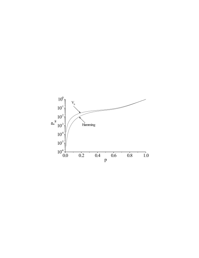
Figure 5: Comparison of $P_{{\rm ue}}(V_{0},p)$ and $P_{{\rm ue}}(H,p)$ for $n=15$.

VI Heuristic approximations

The lower bound discussed in the previous section neglects all the events caused by $j$ errors where $5\leq j\leq i-5$. As a consequence, the approximation is good for small $p$ (and, symmetrically, for large $p$) but it becomes less and less reliable in the central region of $p$ values.

Another approach is to find some good approximation of $A_{i,j}^{(0)}$ by some heuristic argument. By (6)-(8), we only have to consider $j$ in the range $2\leq j\leq i/2$.

First, we observe that a vector ${\mathbf{e}}$ of weight $j$ is contained in ${n-j\choose i-j}$ vectors ${\mathbf{x}}$ of weight $i$. Each such vector ${\mathbf{x}}$ is contained in some code $V_{g}$. Since there are $A_{j}^{(0)}$ vectors ${\mathbf{e}}\in V_{0}^{\prime}$ of weight $j$, we get

$${n-j\choose i-j}A_{j}^{(0)}=\sum_{g=0}^{n}A_{i,j}^{(g)}.$$ (13)

Now (and this is the heuristic argument), we assume that the ratio between the number of undetectable errors of weight $j$ in $V_{g}$ and the overall number of errors of weight $j$ (given by (13)), starting from codewords ${\mathbf{x}}$ of weight $i$, is approximately equal to the ratio between the number of codewords of weight $i$ in $V_{g}$ and the total number of codewords of weight $i$. In particular, for $V_{0}$, this means to assume:

$$\frac{A_{i,j}^{(0)}}{{n-j\choose i-j}A_{j}^{(0)}}\approx\frac{A_{i}^{(0)}}{{n\choose i}}.$$

Hence, under our assumption, we get

$$A_{i,j}^{(0)}\approx\frac{{n-j\choose i-j}}{{n\choose i}}A_{j}^{(0)}A_{i}^{(0)}.$$ (14)

This approximation can be computed using (2). We observe that for $i=n$, we have equality in (14), that is,

$$A_{n,j}^{(0)}=A_{j}^{(0)}A_{n}^{(0)}.$$

Even more simply, as an alternative to using (2), one can combine (14) with the approximations for $A_{i}^{(0)}$ and $A_{j}^{(0)}$ given by (3) and get

$$A_{i,j}^{(0)}\approx\frac{1}{(n+1)^{2}}{n-j\choose i-j}{n\choose j}=\frac{1}{(n+1)^{2}}{n\choose i}{i\choose j}$$ (15)

for $2\leq j\leq i-2$ while, using (7), we get

$$A_{i,i}^{(0)}\approx\frac{1}{(n+1)}{n\choose i}.$$ (16)

Finally, in the case of even $n$, using (11), we get

$$A_{n,j}^{(0)}\approx\frac{1}{(n+1)}{n\choose j}.$$ (17)

The heuristic argument is justified by a number of simulation evidences. Just as an example, in Fig. 6 we show the comparison between the exact values of $A_{i,j}^{(0)}$ and those derived from the heuristic approximation, as a function of $i$, for $n=20$ and some values of $j$, namely $j=i$ (i.e., using (16) for the heuristic approximation), and $j=2,3,4$ ((i.e., using (15) and (17) for the heuristic approximation). The heuristic values have been interpolated by continuous lines for the sake of readability. The figure shows that the agreement between the approximated values and the exact ones is very good. Though referred to a particular case, this conclusion is quite general, and we have verified it also for the other values of $j$ and for different $n$ (for example, $n=25$). From a theoretical point of view, the heuristic argument can be seen as an instance of the “random coding” approach, that has been also used recently, over the Z-channel, to extend the concept of Maximum Likelihood decoding [14]. As the practical significance of random coding increases with the size of the code, we can foresee that the goodness of the heuristic argument is confirmed for larger values of $n$.

Figure 6: Comparison between the exact values of $A_{i,j}^{(0)}$ (dots) and those derived from the heuristic approximation (continuous lines) as a function of $i$ for $n=20$ and some values of $j$.

In practice, the best approach for moderate $n$ is to determine some $A_{i,j}^{(0)}$ explicitly, as outlined above, e.g. for $j\leq 4$, combined with (6) and (7), and to use one of the approximations in (14) and (15) for the remaining $A_{i,j}^{(0)}$. For $n=25$ we have done this, with exact values for $A_{i,j}^{(0)}$ and $A_{i,i-j}^{(0)}$ for $0\leq j\leq 4$, and with the approximation in (14) for the remaining $A_{i,j}^{(0)}$. For this case, the exact values and the approximations are very close, and if we draw both in a graph it is not possible to distinguish between them. The maximal percentage difference between the curves is less than 0.065%; the maximum occurs in the neighborhood of $p=0.5$.

For our heuristic approximation given in terms of the binomial coefficients, we can find a closed formula. The analytical details are given in Appendix I; using the approximations in (15) and (16) we get the following expression:

$$\left(n+1\right)^{2}\#V_{0}P_{\mathrm{ue}}^{\mathrm{h}}\left(V_{0},p\right)$$ (18)

$$= 2^{n}-(2-p)^{n}-np(2-p)^{n-1}$$

$$+2np(1+p)^{n-1}-2np-n(n-1)p^{2}.$$

It is easy to see that, for $n$ sufficiently large and except for $p$ close to zero or one, at the right side, the first term is much larger than the others. So, taking into account that $(n+1)^{2}\#V_{0}\approx(n+1)2^{n}$, we have $P_{{\rm ue}}^{{\rm h}}(V_{0},p)\approx\frac{1}{n+1}$. This statement can be made more precise. We also see that

$$P_{{\rm ue}}^{{\rm h}}(V_{0},0)=0=P_{{\rm ue}}(V_{0},0)$$

and

$$P_{{\rm ue}}^{{\rm h}}(V_{0},1)=1-\frac{1}{\#V_{0}}=P_{{\rm ue}}(V_{0},1).$$

Now, let us consider the derivative of $P_{{\rm ue}}^{{\rm h}}(V_{0},p)$. With simple algebra, we get

$$(n+1)^{2}\#V_{0}\frac{d}{dp}P_{{\rm ue}}^{{\rm h}}(V_{0},p)$$

$$= n(2-p)^{n-1}-\Bigl{[}n(2-p)^{n-1}-n(n-1)p(2-p)^{n-2}\Bigr{]}$$

$$+\Bigl{[}2n(1+p)^{n-1}+2n(n-1)p(1+p)^{n-2}\Bigr{]}-2n$$

$$-2n(n-1)p$$

$$= 2n(1+np)\Bigl{[}(1+p)^{n-2}-1\Bigr{]}+n(n-1)p(2-p)^{n-2}$$

$$+2np.$$

In particular, we see that $\frac{d}{dp}P_{{\rm ue}}^{{\rm h}}(V_{0},p)>0$ for all $p\in(0,1)$; hence $P_{{\rm ue}}^{{\rm h}}(V_{0},p)$ is increasing with $p$. Moreover, it is possible to show that $P_{{\rm ue}}^{{\rm h}}(V_{0},p)$ exhibits a nearly flat region on the interval $\Bigl{[}\frac{1}{\sqrt{n}},1-\frac{1}{\sqrt{n}}\Bigl{]}$. This can be proved by considering that, for large $n$, the following approximations hold (see Appendix II for demonstration):

$$P_{\mathrm{ue}}^{\mathrm{h}}\left(V_{0},\frac{1}{\sqrt{n}}\right) \simeq \frac{2^{n}}{\left(n+1\right)^{2}\#V_{0}}\left(1-\sqrt{n}e^{-\frac{\sqrt{n}}{2}-\frac{1}{8}}\right)$$

$$P_{\mathrm{ue}}^{\mathrm{h}}\left(V_{0},1-\frac{1}{\sqrt{n}}\right) \simeq \frac{2^{n}}{\left(n+1\right)^{2}\#V_{0}}\left(1+2ne^{-\frac{\sqrt{n}}{2}-\frac{1}{8}}\right).$$

By using the approximation $\#V_{0}\simeq 2^{n}/(n+1)$ we can obtain:

$$P_{\mathrm{ue}}^{\mathrm{h}}\left(V_{0},1-\frac{1}{\sqrt{n}}\right)-P_{\mathrm{ue}}^{\mathrm{h}}\left(V_{0},\frac{1}{\sqrt{n}}\right)$$

$$\simeq \frac{2^{n}}{\left(n+1\right)^{2}\#V_{0}}\left(2n+\sqrt{n}\right)e^{-\frac{\sqrt{n}}{2}-\frac{1}{8}}\simeq\frac{2n}{n+1}e^{-\frac{\sqrt{n}}{2}-\frac{1}{8}}.$$

Therefore

$$P_{\mathrm{ue}}^{\mathrm{h}}\left(V_{0},1-\frac{1}{\sqrt{n}}\right)-P_{\mathrm{ue}}^{\mathrm{h}}\left(V_{0},\frac{1}{\sqrt{n}}\right)\rightarrow 0$$

for $n\rightarrow\infty$. Combined with the fact that $P_{{\rm ue}}^{{\rm h}}(V_{0},p)$ is increasing, this confirms the existence of a nearly flat region on the interval $\Bigl{[}\frac{1}{\sqrt{n}},1-\frac{1}{\sqrt{n}}\Bigl{]}$. For example, if $n=509$, then $1/\sqrt{n}\simeq 0.044$, and (18) gives

$$P_{{\rm ue}}^{{\rm h}}(V_{0},1/\sqrt{n})\simeq 0.001961,P_{{\rm ue}}^{{\rm h}}(V_{0},1-1/\sqrt{n})\simeq 0.001972.$$

It is interesting to observe that the existence of a nearly flat region for the probability of undetected error can be also proved, in general terms, for any linear (or even non linear) code over the BSC. Demonstration is given in Appendix III.

For Hamming codes, in particular, the existence of a nearly flat region in the function $P_{\mathrm{ue}}^{\mathrm{BSC}}(H,p)$, given by (12), on the interval $\Bigl{[}\frac{1}{\sqrt{n}},1-\frac{1}{\sqrt{n}}\Bigl{]}$, can be proved through similar arguments as those used above for the VT codes. In this case, the derivative of the probability of undetected error can be expressed as follows [11, p. 44]:

$$\frac{dP_{{\rm ue}}^{{\rm BSC}}(H,p)}{dp} = n\left[(1-p)^{n-1}-(1-2p)^{(n-1)/2}\right]$$

$$= n\left\{\left[(1-p)^{2}\right]^{(n-1)/2}-(1-2p)^{(n-1)/2}\right\}.$$

Since $\left(1-p\right)^{2}\geq\left(1-2p\right)$, it follows that

$$\frac{dP_{{\rm ue}}^{{\rm BSC}}(H,p)}{dp}>0\mbox{ for all }p\in(0,1),$$

and so $P_{{\rm ue}}^{{\rm BSC}}(H,p)$ is increasing with $p$. If we consider the values of $P_{{\rm ue}}^{{\rm BSC}}(H,p)$ for $p=\frac{1}{\sqrt{n}}$ and $p=1-\frac{1}{\sqrt{n}}$, we can prove that, for large $n$, the following approximations hold:

$$P_{\mathrm{ue}}^{\mathrm{BSC}}\left(H,\frac{1}{\sqrt{n}}\right) \simeq \frac{1+ne^{-\sqrt{n}-1}\left(1-\sqrt{e}\right)}{n+1}$$

$$P_{\mathrm{ue}}^{\mathrm{BSC}}\left(H,1-\frac{1}{\sqrt{n}}\right) \simeq \frac{1+ne^{-\sqrt{n}-1}}{n+1}.$$

Demonstration is given in Appendix II. It follows that

$$P_{\mathrm{ue}}^{\mathrm{BSC}}\left(H,1-\frac{1}{\sqrt{n}}\right)-P_{\mathrm{ue}}^{\mathrm{BSC}}\left(H,\frac{1}{\sqrt{n}}\right)$$

$$\simeq \frac{n}{n+1}e^{-\sqrt{n}-1}\left(1-1+\sqrt{e}\right)=\frac{n}{n+1}e^{-\sqrt{n}-\frac{1}{2}}.$$

Therefore

$$P_{\mathrm{ue}}^{\mathrm{BSC}}\left(H,1-\frac{1}{\sqrt{n}}\right)-P_{\mathrm{ue}}^{\mathrm{BSC}}\left(H,\frac{1}{\sqrt{n}}\right)\rightarrow 0$$

for $n\rightarrow\infty$. Combined with the fact that $P_{{\rm ue}}^{{\rm BSC}}(H,p)$ is increasing, this confirms the existence of a nearly flat region on the interval $\Bigl{[}\frac{1}{\sqrt{n}},1-\frac{1}{\sqrt{n}}\Bigl{]}$ also in this case. In such region,

$$P_{{\rm ue}}^{{\rm BSC}}(H,p)\approx\frac{1}{n+1}.$$

This is the same approximate value determined above for $P_{{\rm ue}}^{{\rm h}}(V_{0},p)$. However, it is possible to verify that, for a fixed $n$, the extent of the region where $P_{{\rm ue}}^{{\rm BSC}}(H,p)$ is almost constant is larger than that where $P_{{\rm ue}}^{{\rm h}}(V_{0},p)$ is almost constant.

Because of the lack of an explicit formula, it is not possible to demonstrate analytically that the same nearly flat region appears also when the Hamming code is applied over the Z-channel. However, the simulations described in the next section indicate that this is the case. So, assuming this, we can say that, even keeping in mind the different meaning of $p$ over the symmetric and the asymmetric channels, the curves of the probability of undetected error for VT codes and Hamming codes of the same length over the Z-channel and those for Hamming codes over the BSC are almost constant, and practically superposed, in a wide region of the channel error probability.

VII Performance simulation

In the previous section we have shown that the heuristic approach provides a very good approximation for the case of small code lengths. Testing reliability of the heuristic approximation for large lengths, through a comparison with the exact results, is impossible, as the exhaustive analysis becomes too complex just for $n>30$. For large lengths, however, it can be useful to resort to a Monte Carlo like method, that is, to develop a simulator. The simulator replicates the behavior of a “real" system, and gives an estimate of the unknown probability as the ratio between the number of undetected errors and the number of simulated codewords.

A rule must be established to construct the code from the information sequence. The simplest way to convert an information frame into a codeword consists in applying a systematic encoding. Systematic VT codes have been studied in [10]. As reminded in Section V, in a systematic code, every codeword consists of a $k$ bits information vector and an $r$ bits parity check vector. In [10], a systematic encoding procedure for VT codes of length $n$ and $r=\lceil\log_{2}(n+1)\rceil$ was given. This is, basically, the same that is obtained with conventional Hamming codes (see Section V).

The systematic encoding procedure described in [10] is very simple: the $k=n-\lceil\log_{2}(n+1)\rceil$ information bits are set in the positions:

$$I=\left\{1,...,n\right\}\setminus\left\{2^{j}:j=0,1,...,\lceil\log_{2}(n+1)\rceil-1\right\}.$$

$I$ defines a maximal standard information set for the VT code, i.e., it ensures the value of $k$ is maximum. The remaining positions are occupied by the parity check bits, whose values are determined in such a way as to satisfy (1).

In general, the codewords of the systematic code, for a given value of $n$, are a subset of those obtainable through the solution of (1). On the other hand, it is evident that any codeword of $V_{0}$ can be a codeword of the systematic code: in practice, many information sequences can be encoded into more than one codeword of $V_{0}$. As an example, for $n=10$, the information sequence (011001) can be equivalently encoded into (1000110001) or into (0001110101). When using the systematic code, one option should be chosen, when necessary, in order to define the codewords uniquely. For our simulation purposes, however, the goal is to generate the codewords of $V_{0}$ according to a uniform distribution. To this purpose, we do not adopt any selection rule; on the contrary, when an information sequence is randomly generated for transmission over the Z-channel, all its possible encodings are considered. This way, simulation, that for high values of $n$ necessarily corresponds to sampling a subset of $V_{0}$, does not exhibit any “polarization effect" and the simulated scenario strictly resembles that of the analytical model (and the heuristic argument, in particular).

First, we have verified these conjectures by simulating the code with $n=25$, that is the longest code for which we have presented before the exact result; as shown in Fig. 7, the simulated points are everywhere superposed to the exact curve.

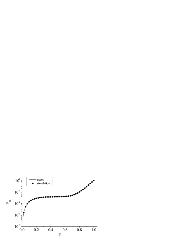
Figure 7: Comparison between the simulated values and the exact curve of $P_{{\rm ue}}(V_{0},p)$ in the case of $n=25$.

Then, and most important, simulation has permitted us to study much longer codes. We have analyzed lengths up to $n=509$ (that corresponds, according with the systematic rule, to $k=500$). In order to ensure a satisfactory statistical confidence level for the simulated $P_{{\rm ue}}(V_{0},p)$, each simulation has been stopped after having found 50000 undetected errors.

The simulated curves for these long codes generally show a wide nearly flat region, for intermediate values of $p$, as expected from the heuristic analysis. Some examples of the numerical results obtained, confirming the above considerations, are given in Table I. For better evidence, in Fig. 8 we have plotted the heuristic approximation and the simulated values for $n=509$. We see that the approximation is excellent also in this case.

TABLE I: Examples of simulated values of $P_{{\rm ue}}(V_{0},p)$ for some values of $n$ and $p$

$p$	$n=36$	$n=67$	$n=127$	$n=247$	$n=509$
0.05	0.00643	0.00742	0.00647	0.00402	0.00195
0.1	0.01503	0.01261	0.00776	0.00403	0.00197
0.15	0.02088	0.01426	0.00785	0.00404	0.00196
0.2	0.02412	0.01463	0.00783	0.00403	0.00196
0.25	0.02573	0.01469	0.00780	0.00403	0.00197
0.3	0.02645	0.01465	0.00780	0.00404	0.00196
0.35	0.02677	0.01467	0.00782	0.00403	0.00196
0.4	0.02692	0.01479	0.00785	0.00404	0.00196
0.45	0.02692	0.01474	0.00780	0.00403	0.00197
0.5	0.02719	0.01469	0.00780	0.00402	0.00196
0.55	0.02729	0.01476	0.00781	0.00400	0.00195
0.6	0.02751	0.01467	0.00780	0.00402	0.00196
0.65	0.02785	0.01468	0.00781	0.00403	0.00196
0.7	0.02932	0.01468	0.00780	0.00401	0.00197
0.75	0.03402	0.01476	0.00779	0.00403	0.00196
0.8	0.04683	0.01553	0.00782	0.00404	0.00195
0.85	0.08159	0.01962	0.00793	0.00400	0.00197
0.9	0.17323	0.04481	0.00928	0.00405	0.00196
0.95	0.40865	0.19059	0.04674	0.00591	0.00195

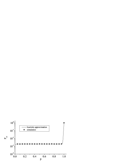
Figure 8: Comparison between the simulated values of $P_{{\rm ue}}(V_{0},p)$ and the (heuristic) approximation $P_{{\rm ue}}^{{\rm h}}(V_{0},p)$ for $n=509$.

Finally, we can compare the performance of VT codes with that of Hamming codes, with the same code length, most of all for demonstrating the (quasi) coincidence of the nearly constant value. An example, for $n=127$, is shown in Fig. 9: the continuous line represents $P_{{\rm ue}}^{{\rm h}}(V_{0},p)$, while dots represent some simulated points for $P_{{\rm ue}}(H,p)$. As expected, also the latter curve exhibits a wide nearly flat region, and the value of both functions are practically the same in this region. Moreover, this value is also approximately equal to $1/(n+1)=0.0078125$ that, as proved in Section VII, provides the $P_{{\rm ue}}^{{\rm BSC}}(H,p)$ almost everywhere, except for values of $p$ close to zero or close to one.

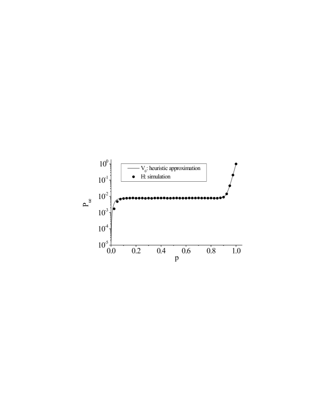
Figure 9: Comparison between the simulated values of $P_{{\rm ue}}(H,p)$ and the (heuristic) approximation $P_{{\rm ue}}^{{\rm h}}(V_{0},p)$ for $n=127$.

VIII Conclusion

This paper is a first attack on the problem of evaluating the undetected error probability of Varshamov-Tenengol’ts codes. We have presented some methods that allow us to obtain exact results (for short codes) and heuristic and simulated approximate results (for long codes). We have shown that the proposed heuristic approximation is excellent for small $n$, and very good even for large $n$.

We have verified that the probability of undetected error is almost constant in a wide region of values of the channel error probability, and this region becomes larger and larger for increasing $n$. Such a behavior is common to other codes, over the Z-channel, and can be found even in the case of a generic, linear or non-linear, code over the symmetric channel. Thus, we can conclude that, except for the region of a channel error probability close to zero or one, the probability of undetected error tends to assume the same value, approximately equal to the reciprocal of the code length, independently of the code and of the symmetry properties of the channel. Further work should be advisable to confirm these conclusions on other codes. In regard to VT codes, though their error detection properties seem disclosed from the analytical and numerical approaches proposed in this paper, it remains a valuable task to find closed form expressions for the quantities $A_{i,j}^{(0)}$, or even $A_{i,j}^{(g)}$ for all $g$, in such a way as to be able to compute the undetected error probability exactly for any code length.

Appendix I: On the heuristic approximation $P_{{\rm ue}}^{{\rm h}}(V_{0},p)$

Let us consider (5), by assuming $g=0$ and replacing the approximation (16) for $j=i$ and (15) for $j\neq i$; so, we get:

$$\#V_{0}P_{{\rm ue}}^{{\rm h}}(V_{0},p)$$

$$= \sum_{i=2}^{n}\frac{1}{n+1}{n\choose i}p^{i}$$

$$+\sum_{i=4}^{n}\sum_{j=2}^{i-2}\frac{1}{(n+1)^{2}}{n\choose i}{i\choose j}p^{j}(1-p)^{i-j}.$$

Through simple algebra, we have:

$$(n+1)^{2}\#V_{0}P_{{\rm ue}}^{{\rm h}}(V_{0},p)$$

$$= (n+1)^{2}\sum_{i=2}^{n}\frac{1}{n+1}{n\choose i}p^{i}$$

$$+(n+1)^{2}\sum_{i=4}^{n}\sum_{j=2}^{i-2}\frac{1}{(n+1)^{2}}{n\choose i}{i\choose j}p^{j}(1-p)^{i-j}$$

$$= (n+1)\sum_{i=2}^{n}{n\choose i}p^{i}+\sum_{i=4}^{n}{n\choose i}\sum_{j=2}^{i-2}{i\choose j}p^{j}(1-p)^{i-j}$$

$$= (n+1)\sum_{i=2}^{n}{n\choose i}p^{i}$$

$$+\sum_{i=4}^{n}{n\choose i}\Bigl{[}1-(1-p)^{i}-ip(1-p)^{i-1}\Bigr{.}$$

$$\qquad\Bigl{.}-ip^{i-1}(1-p)-p^{i}\Bigr{]}$$

$$= (n+1)\Bigl{[}(1+p)^{n}-1-np\Bigr{]}$$

$$+\Bigl{[}2^{n}-1-n-{n\choose 2}-{n\choose 3}\Bigr{]}$$

$$-\Bigl{[}(2-p)^{n}-1-n(1-p)\Bigr{.}$$

$$\Bigl{.}\qquad-{n\choose 2}(1-p)^{2}-{n\choose 3}(1-p)^{3}\Bigr{]}$$

$$-np\Bigl{[}(2-p)^{n-1}-1-(n-1)(1-p)\Bigr{.}$$

$$\Bigl{.}\qquad-{n-1\choose 2}(1-p)^{2}\Bigr{]}$$

$$-n(1-p)\Bigl{[}(1+p)^{n-1}-1-(n-1)p-{n-1\choose 2}p^{2}\Bigr{]}$$

$$-\Bigl{[}(1+p)^{n}-1-np-{n\choose 2}p^{2}-{n\choose 3}p^{3}\Bigr{]}$$

$$= 2^{n}-(2-p)^{n}-np(2-p)^{n-1}$$

$$+2np(1+p)^{n-1}-2np-n(n-1)p^{2}.$$

Hence

$$(n+1)^{2}\#V_{0}P_{{\rm ue}}^{{\rm h}}(V_{0},p)$$

$$= 2^{n}-(2-p)^{n}-np(2-p)^{n-1}$$

$$+2np(1+p)^{n-1}-2np-n(n-1)p^{2}.$$

This is the expression given in (18) in Section VI.

Appendix II: Approximate values of $P_{{\rm ue}}$ for $p=\frac{1}{\sqrt{n}}$ and $p=1-\frac{1}{\sqrt{n}}$.

Let us consider, at first, the expression of $P_{\mathrm{ue}}^{\mathrm{h}}(V_{0},p)$, given by (18), for the approximate probability of undetected error of VT codes over the Z-channel. For $p=\frac{1}{\sqrt{n}}$, $P_{\mathrm{ue}}^{\mathrm{h}}(V_{0},p)$ takes the value

$$\left(n+1\right)^{2}\#V_{0}P_{\mathrm{ue}}^{\mathrm{h}}\left(V_{0},\frac{1}{\sqrt{n}}\right)$$ (19)

$$= 2^{n}-\left(2-\frac{1}{\sqrt{n}}\right)^{n}-n\frac{1}{\sqrt{n}}\left(2-\frac{1}{\sqrt{n}}\right)^{n-1}$$

$$+2n\frac{1}{\sqrt{n}}\left(1+\frac{1}{\sqrt{n}}\right)^{n-1}$$

$$-2n\frac{1}{\sqrt{n}}-n\left(n-1\right)\frac{1}{n}.$$

Considering that $\left(2-\frac{1}{\sqrt{n}}\right)^{n}=2^{n}\left(1-\frac{1}{2\sqrt{n}}\right)^{n}$, we can adopt an approximate expression for such term. In fact, since $0<\frac{1}{2\sqrt{n}}\leq\frac{1}{2}$, the Taylor expansion

$$\mathrm{ln}\left(1-\frac{1}{2\sqrt{n}}\right)=-\frac{1}{2\sqrt{n}}-\frac{1}{8n}-\frac{1}{24n^{3/2}}-\cdots$$

can be used. This way, we obtain

$$\left(2-\frac{1}{\sqrt{n}}\right)^{n} = 2^{n}e^{n\mathrm{ln}\left(1-\frac{1}{2\sqrt{n}}\right)}$$

$$= 2^{n}e^{-\frac{\sqrt{n}}{2}-\frac{1}{8}+O\left(\frac{1}{\sqrt{n}}\right)}$$

$$\simeq 2^{n}e^{-\frac{\sqrt{n}}{2}-\frac{1}{8}}.$$

when $n\rightarrow\infty$.

Similarly, we can obtain $\left(2-\frac{1}{\sqrt{n}}\right)^{n-1}\simeq 2^{n}e^{-\frac{\sqrt{n}}{2}-\frac{1}{8}}$ and $\left(1+\frac{1}{\sqrt{n}}\right)^{n-1}\simeq e^{\sqrt{n}-\frac{1}{2}}$; so (19) can be rewritten as follows:

$$(n+1)^{2}\#V_{0}P_{\mathrm{ue}}^{\mathrm{h}}\left(V_{0},\frac{1}{\sqrt{n}}\right)$$

$$\simeq 2^{n}-2^{n}e^{-\frac{\sqrt{n}}{2}-\frac{1}{8}}-\sqrt{n}2^{n}e^{-\frac{\sqrt{n}}{2}-\frac{1}{8}}$$

$$+2\sqrt{n}e^{\sqrt{n}-\frac{1}{2}}-2\sqrt{n}-n+1.$$

Considering only the leading terms, we have

$$P_{\mathrm{ue}}^{\mathrm{h}}\left(V_{0},\frac{1}{\sqrt{n}}\right)\simeq\frac{2^{n}}{\left(n+1\right)^{2}\#V_{0}}\left(1-\sqrt{n}e^{-\frac{\sqrt{n}}{2}-\frac{1}{8}}\right),$$

when $n\rightarrow\infty$.

We can adopt the same approach in order to obtain an estimate of $P_{\mathrm{ue}}^{\mathrm{h}}(V_{0},1-\frac{1}{\sqrt{n}})$. We get

$$(n+1)^{2}\#V_{0}P_{\mathrm{ue}}^{\mathrm{h}}\left(V_{0},1-\frac{1}{\sqrt{n}}\right)$$

$$= 2^{n}-\left(1+\frac{1}{\sqrt{n}}\right)^{n}-n\left(1-\frac{1}{\sqrt{n}}\right)\left(1+\frac{1}{\sqrt{n}}\right)^{n-1}$$

$$+2n\left(1-\frac{1}{\sqrt{n}}\right)\left(2-\frac{1}{\sqrt{n}}\right)^{n-1}-2n\left(1-\frac{1}{\sqrt{n}}\right)$$

$$-n\left(n-1\right)\left(1-\frac{1}{\sqrt{n}}\right)^{2}.$$

Using the approximations above, this can be rewritten as follows:

$$(n+1)^{2}\#V_{0}P_{\mathrm{ue}}^{\mathrm{h}}\left(V_{0},1-\frac{1}{\sqrt{n}}\right)$$

$$\simeq 2^{n}-\left(n+1-\sqrt{n}\right)e^{\sqrt{n}-\frac{1}{2}}$$

$$+2\left(n-\sqrt{n}\right)\left(2^{n}e^{-\frac{\sqrt{n}}{2}-\frac{1}{8}}-1\right)$$

$$-n(n-1)\left(1-\frac{1}{\sqrt{n}}\right)^{2}.$$

Considering only the leading terms, we have

$$P_{\mathrm{ue}}^{\mathrm{h}}\left(V_{0},1-\frac{1}{\sqrt{n}}\right)\simeq\frac{2^{n}}{\left(n+1\right)^{2}\#V_{0}}\left(1+2ne^{-\frac{\sqrt{n}}{2}-\frac{1}{8}}\right)$$

when $n\rightarrow\infty$.

A quite similar approach can be applied to the probability of undetected error of Hamming codes, over the BSC, as given by (12). In particular, we have:

$$P_{\mathrm{ue}}^{\mathrm{BSC}}\left(H,\frac{1}{\sqrt{n}}\right)$$

$$= \frac{1}{n+1}+\frac{n}{n+1}\left(1-\frac{2}{\sqrt{n}}\right)^{\frac{n+1}{2}}-\left(1-\frac{1}{\sqrt{n}}\right)^{n}.$$

As, for large $n$, $\left(1-\frac{2}{\sqrt{n}}\right)^{\frac{n+1}{2}}\simeq e^{-\sqrt{n}-1}$ and $\left(1-\frac{1}{\sqrt{n}}\right)^{n}\simeq e^{-\sqrt{n}-\frac{1}{2}}$, this implies the following approximation:

$$P_{\mathrm{ue}}^{\mathrm{BSC}}\left(H,\frac{1}{\sqrt{n}}\right) \simeq \frac{1+ne^{-\sqrt{n}-1}-\left(n+1\right)e^{-\sqrt{n}-\frac{1}{2}}}{n+1}$$

$$\simeq \frac{1+ne^{-\sqrt{n}-1}\left(1-\sqrt{e}\right)}{n+1}.$$

At the point $p=1-\frac{1}{\sqrt{n}}$, instead we have:

$$P_{\mathrm{ue}}^{\mathrm{BSC}}\left(H,1-\frac{1}{\sqrt{n}}\right)=\frac{1}{n+1}\left[1+n\left(1-\frac{2}{\sqrt{n}}\right)^{\frac{n+1}{2}}\right]-n^{-\frac{n}{2}}$$

having taken into account that $(n+1)/2$ is always even. Moreover, considering that $\left(1-\frac{2}{\sqrt{n}}\right)^{\frac{n+1}{2}}\simeq e^{-\sqrt{n}-1}$, we have:

$$P_{\mathrm{ue}}^{\mathrm{BSC}}\left(H,1-\frac{1}{\sqrt{n}}\right)\simeq\frac{1+ne^{-\sqrt{n}-1}}{n+1}.$$

Appendix III: On the probability of undetected error of binary codes over the symmetric channel

Let $C$ be a binary $(n,M,d)$ code (it can be linear or non-linear). By [11, p. 44, Theorem 2.4],

$$P_{{\rm ue}}(C,p)=\frac{M}{2^{n}}\Bigl{\{}1+\sum_{i=d^{\perp}}^{n}A_{i}^{\perp}(1-2p)^{i}\Bigr{\}}-(1-p)^{n}$$

where $A_{i}^{\perp}$ is the dual weight distribution (the MacWilliams transform of the weight distribution) of the code (for a linear code this is the weight distribution of the dual code) and $d^{\perp}$ the dual distance (that is, the least $i>0$ such that $A_{i}^{\perp}\neq 0$).

Therefore,

$$\frac{d{P_{{\rm ue}}(C,p)}}{dp}=-\frac{M}{2^{n-1}}\sum_{i=d^{\perp}}^{n}iA_{i}^{\perp}(1-2p)^{i-1}+n(1-p)^{n-1}.$$ (20)

It is known that $A_{i}^{\perp}\geq 0$ (see [11, p. 16, Corollary 1.1]). Since $|1-2p|\leq 1$ for $p\in[0,1]$, we get

$$-(1-2p)^{i-1}\leq|1-2p|^{i-1}\leq|1-2p|^{d^{\perp}-1}$$

for $i\geq d^{\perp}$. Further, it is known (see [11, p. 14, Theorem 1.4]) that

$$\frac{M}{2^{n-1}}\sum_{i=d^{\perp}}^{n}iA_{i}^{\perp}=n-A_{1}\leq n.$$

Hence, from (20) we get

$$\frac{d{P_{{\rm ue}}(C,p)}}{dp} \leq n(1-p)^{n-1}+\frac{M}{2^{n-1}}\sum_{i=d^{\perp}}^{n}iA_{i}^{\perp}|1-2p|^{d^{\perp}-1}$$

$$\leq n(1-p)^{n-1}+n|1-2p|^{d^{\perp}-1}.$$

Similarly, we get

$$\frac{dP_{{\rm ue}}(C,p)}{dp}\geq n(1-p)^{n-1}-n|1-2p|^{d^{\perp}-1}.$$

The term $n(1-p)^{n-1}$ is close to zero for $p$ removed from zero and one, for example for $1/\sqrt{n}\leq p\leq 1-1/\sqrt{n}$.

The term $n|1-2p|^{d^{\perp}-1}$ is clearly small for $p$ close to $1/2$. If $d^{\perp}$ is of some size, it is also small over some range around $p=1/2$. The bounds above show that $\frac{d{P_{{\rm ue}}(C,p)}}{dp}$ is also close to zero, and hence,

$$P_{{\rm ue}}(C,p)\approx P_{{\rm ue}}(C,1/2)=(M-1)/2^{n}$$

over this range.

References

- [1] T. R. N. Rao and E. Fujiwara, Error-Control Coding for Computer Systems, Prentice-Hall Int. 1989.
- [2] H. Kaneko and E. Fujiwara, “A class of M-ary asymmetric symbol error correcting codes for data entry devices”, IEEE Trans. Computers, vol. 53, no. 2, 159–167, 2004.
- [3] X. Zhang, S. Zhou, and P. Willet, “Loading for parallel binary channels”, IEEE Trans. Commun., vol. 54, no. 1, 51–55, 2006.
- [4] T. Kløve, Error Correcting Codes for the Asymmetric Channel, University of Bergen, 1995. Available at http://www.ii.uib.no/torleiv/Papers/index.html
- [5] T. Etzion, “New Lower Bounds for Asymmetric and Unidirectional Codes”, IEEE Trans. Inform. Theory, vol. 37, no. 6, pp. 1696–1704, 1991.
- [6] V. P. Shilo “New Lower Bounds of the Size of Error-Correcting Codes for the Z-Channel”, Cybernetics and Systems Analysis, vol. 38, no. 1, pp. 13–16, 2002.
- [7] R. R. Varshamov and G. M. Tenengol’ts, “Correcting code for single asymmetric errors”, Avtomatika i Telemekhanika, vol. 26, no. 2, pp. 288–292, 1965 (in Russian), translation: Automation and Remote Contr., vol. 26, pp. 286–290.
- [8] L. E. Mazur, “Correcting codes for asymmetric errors”, Problemy Peredachi Informatsii, vol. 10, no. 4, pp. 40–46, 1974 (in Russian), translation: Problems of Information Transmission, vol. 10, pp. 308–312.
- [9] T. Helleseth and T. Kløve, “On group-theoretic codes for asymmetric channels”, Inform. and Control, vol. 49, pp. 1-9, 1981.
- [10] K. A. S. Abdel-Ghaffar and H. C. Ferreira, “Systematic encoding of the Varhamov-Tenengol’ts codes and the Constantin-Rao codes”, IEEE Trans. Inform. Theory, vol. 44, no. 1, pp. 340–345, 1998.
- [11] T. Kløve, Codes for Error Detection, World Scientific, 2007.
- [12] A. Kuznetsov, F. Swarts, A. J. Han Vinck, and H. C. Ferreira, “On the undetected error probability of linear block codes on channels with memory”, IEEE Trans. Inform. Theory, vol. 42, no. 1, pp. 303–309, 1996.
- [13] S. Lin, D. J. Costello, Error Control Coding, Pearson Education Int., Second Edition, 2004.
- [14] A. Barbero, P. Ellingsen, S. Spinsante, and Ø. Ytrehus, “Maximum likelihood decoding of codes on the Z-channel”, Proc. IEEE International Conference on Communications (ICC 2006), Istanbul, Turkey, 11-15 June 2006, vol. 3, pp. 1200-1205.