On Signatures of Atmospheric Features in Thermal Phase Curves of Hot Jupiters

Abstract

Turbulence is ubiquitous in Solar System planetary atmospheres. In hot Jupiter atmospheres, the combination of moderately slow rotation and thick pressure scale height may result in dynamical weather structures with unusually large, planetary-size scales. Using equivalent-barotropic, turbulent circulation models, we illustrate how such structures can generate a variety of features in the thermal phase curves of hot Jupiters, including phase shifts and deviations from periodicity. Such features may have been spotted in the recent infrared phase curve of HD 189733b. Despite inherent difficulties with the interpretation of disk-integrated quantities, phase curves promise to offer unique constraints on the nature of the circulation regime present on hot Jupiters.

1 Introduction

Just over two years ago the Spitzer Space Telescope was used for the first direct detections of light from extrasolar planets (Charbonneau et al., 2005; Deming et al., 2005), heralding the birth of a new field of observational astronomy: the characterization of exoplanet atmospheres. So far these direct measurements are only possible for the shortest period “hot Jupiter” exoplanets, as these planets are heated enough to radiate $\sim 10^{-3}$ of their parent stars’ infrared emission, making the planet’s component of the signal just separable from the stellar component. In the last couple of years, many new results have emerged in this field, including several more infrared direct detections of hot Jupiters (and a Neptune!) through secondary eclipse measurements (Deming et al., 2006, 2007b; Harrington et al., 2007), measurements of infrared emission spectra (Grillmair et al., 2007; Richardson et al., 2007), and orbital phase variation from the day-night temperature contrasts of eclipsing and non-eclipsing planets (Harrington et al., 2006; Cowan et al., 2007; Knutson et al., 2007). Further exciting results are expected from the last round of cryogenic Spitzer observations, the “warm Spitzer” phase (Deming et al., 2007a), and continuing on with the vastly increased photometric sensitivity of the James Webb Space Telescope (JWST). The launch of JWST will enable high precision measurements and the acquisition of detailed information about the atmospheres of these planets, including the ability to use the known geometry of eclipsing systems to make resolved maps of their day sides (Williams et al., 2006; Rauscher et al., 2007b).

As the number of directly observed systems continues to grow, it is becoming increasingly apparent that not all hot Jupiters are alike. Differences in planetary radii, brightness temperatures or inferred efficiencies of heat redistribution from permanent day sides to cold night sides have led to theoretical speculations on possible ways to subclassify hot Jupiters (Burrows et al., 2007; Fortney et al., 2007; Hansen & Barman, 2007). Perhaps we should not be surprised to discover diversity in these systems (see, e.g., Redfield et al., 2007) since even our own Solar System planets exhibit a wide range of atmospheric conditions. For example, it is currently not well understood what sets the wind speeds at cloud-deck level on the Solar System gas giants. Since atmospheric circulation can be largely driven by insolation, one might expect those planets closer to the Sun to experience stronger winds, but the fact that Neptune receives much less solar illumination than Jupiter and yet has faster winds illustrates how misleading simple arguments may be when applied to these complex, nonlinear flows (Cho et al. 2008; see review by Showman et al. 2007).

Even a thorough understanding of the atmospheric dynamics of the planets in the Solar System would not necessarily allow us to extrapolate to hot Jupiters, which are characterized by a very different atmospheric regime. These presumably tidally locked, short-period planets experience intense stellar irradiation on their constant day sides, much in excess of the internally generated heat flux, while their night sides remain in perpetual shadow. In addition, based on their relatively slow rotation periods, dynamical arguments suggest that large scale atmospheric structures can form on these planets (Cho et al., 2003; Menou et al., 2003; Showman & Guillot, 2002), in contrast to the many thin jets and smaller structures observed on Jupiter, for example. Given this unusual combination of asymmetric heating and slow rotation, there have been several recent attempts to model the atmospheric flow on hot Jupiters (Showman & Guillot, 2002; Cho et al., 2003, 2008; Cooper & Showman, 2005, 2006; Fortney et al., 2006; Langton & Laughlin, 2007; Dobbs-Dixon & Lin, 2007, see review by Showman et al. 2007).

The combination of strong external irradiation (which promotes vertical static stability), moderately slow rotation and large pressure scale heights in hot Jupiter atmospheres results in Rossby deformation radii comparable to or larger than the planetary radii themselves (Showman & Guillot, 2002; Cho et al., 2003; Menou et al., 2003; Showman et al., 2007). The Rossby deformation radius acts as a limiting scale for dynamics in a rotating stratified flow. It sets the typical horizontal size of large vortices in a turbulent atmosphere and determines the scale of the most unstable baroclinic modes. The large deformation radii in hot Jupiter atmospheres may thus limit the importance of baroclinic instabilities and favor a largely barotropic atmospheric flow.

These considerations led Cho et al. (2003, 2008) to apply the two-dimensional, equivalent-barotropic formulation of the primitive equations of meteorology (Salby, 1989) to hot Jupiter atmospheres. This vertically integrated formulation emphasizes the quasi-two dimensional, barotropic nature of the flow. While only adiabatic simulations have been reported so far, a great advantage of the equivalent-barotropic model is that small horizontal scales are resolved in a fully turbulent flow (see, e.g., Cho & Polvani, 1996, for turbulent energy spectra). An additional advantage of this approach is that the set of physical and numerical model parameters is limited and it includes the unknown magnitude of global average wind speed which is treated as an input parameter (Cho et al., 2003, 2008). This allows us to perform an analysis in which we explore a large range of possible equivalent-barotropic flows for hot Jupiter atmospheres and study how these diverse flows may translate into a diversity of thermal phase curves for hot Jupiters.

We begin by describing the models used and our method for computing phase curves in $\S$ 2, move on to discuss predicted model phase curves in $\S$ 3, consider implications for current and future observations in $\S$ 4, and finally conclude in $\S$ 5.

2 Method

We use the adiabatic, equivalent-barotropic model of Cho et al. (2003, 2008) for the planet HD 209458b throughout our analysis. Our main results for thermal phase curves do not strongly depend on the specific planetary parameters adopted—as long as one is concerned with hot Jupiters of the same, broad dynamical class as HD 209458b (see, e.g., Menou et al., 2003). The reader is referred to Cho et al. (2008) for a detailed description of the circulation model. Briefly, the stellar radiative forcing imposes a steady day-night temperature difference on the flow. In the adiabatic equivalent-barotropic model, this forcing is represented by a forced bending of the model’s bottom boundary surface, with a specified bend amplitude $\eta$. This corresponds to a maximum day-night temperature variation of amplitude $\Delta T=\pm\eta\bar{T}$, where $\bar{T}$ is the average equivalent temperature of the modeled layer. The pre-existing background flow, with a prescribed average global wind speed, $\bar{U}$, produces temperature variations, which are superimposed on those due to the steady day-night difference. The combined temperature range covered by each model, as well as the range due to radiative forcing only (case $\bar{U}=0$), are given in Table 1. The model runs have been performed at T63 spectral resolution (equivalent to a fully-resolved 192 $\times$ 96 longitude-latitude grid), which has been found to be sufficient to capture the formation of dominant atmospheric structures (Rauscher et al., 2007a). Following the initialization procedure described in Cho et al. (2003, 2008), each run has been allowed to relax for 40 planetary orbits, after which we output a snapshot of the temperature structure on the planet, 100 times per orbit, for the next 60 orbits.

We create the phase curves presented here by rotating each temperature map to the appropriate viewing orientation for its orbital phase angle and assumed inclination, and orthographically projecting it onto a two dimensional disk. Unless otherwise specified, a $90$^o inclination (edge-on orientation) is assumed by default. We sample the disk with a grid of $[r=20,\theta=40]$ resolution. We solve for three values of emergent flux from each disk element area: a bolometric value $\propto T^{4}$, and Spitzer band fluxes calculated either from a blackbody spectrum based on the local temperature $T$ or a spectral model interpolated from a grid of cloudless 1-D radiative transfer calculations (Seager et al., 2005). As we shall see, our main conclusions depend only weakly on the specific emission model adopted. After obtaining the flux, we integrate over the disk, weighting the emergent flux from each grid point by its relative area on the disk. Our procedure is similar to that adopted in Rauscher et al. (2007a).

We performed resolution tests of our phase curve analysis, both in the number of temperature maps sampled per orbit and the number of grid elements used to sample each map. For computational speed, we use $[r=20,\theta=40]$ as the lowest possible resolution that is immune to noise from under-sampling. The phase curves produced using this resolution are accurate to within a few percent of those produced at higher resolutions. Similarly, we find that by sampling the temperature map of the planet 50 times per orbit, we are able to adequately track the orbital flux variation without losing details in the structure of the phase curve. We have also found that 10 orbits are sufficient to sample the variable patterns seen in the phase curves, making it unnecessary to analyze the full 60 orbits of our model outputs.

3 Phase Curves from Equivalent-Barotropic Models

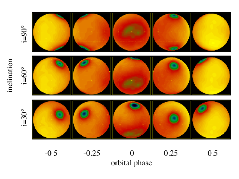
Figure 4: Snapshots of the apparent temperature field in the model with $\eta=0.10$, $\bar{U}=800$ m s^-1, as it rotates through one orbit. Temperatures range from 700 to 1400K. From left to right, the central longitudes are: 0^o (substellar; phase $-0.5$), 90^o, 180^o (antistellar; phase $0$), 270^o, and 360^o. The maps in the top row are shown at an inclination of 90^o (edge-on), the middle ones at 60^o and the bottom ones at 30^o. As the inclination of the system is titled away from edge-on orientation, the cold circumpolar vortices assume a more central location on the apparent planetary disk, so that they affect more strongly the disk-integrated thermal emission. At the same time, more equal areas of the hot day side and cool night side are visible, which decreases the amplitude of the regular peak-trough pattern in the phase curves. [See the electronic edition of the Journal for a color version of this figure.]

The temperature structures predicted by the equivalent-barotropic model consist of two superimposed components: a global day-night “fixed” temperature gradient (the forced bending—see § 2) whose strength depends on the imposed radiative forcing (via the parameter $\eta$), and a variable pattern of weather features created by atmospheric winds. The most prominent weather features are cold circumpolar vortices whose strength (vorticity) increases with higher values of $\bar{U}$. The vortices rotate around the poles with a period comparable, but not equal, to the spin (=orbital) period of the planet. While these vortices are the weather features that most strongly affect the emitted thermal flux in our models, other large scale, possibly transient, features generally exist in an atmosphere. For example, in the models presented here we observe a broader warm area that develops on the side of the planet opposite from the circumpolar vortices, and on occasion cold transient features that develop on the night side. These features constitute the weather on these model planets. Figure 4 shows temperature snapshots for the $\eta=0.10$, $\bar{U}$ = 800 m s^-1 model, exemplifying the type of weather features that develop. Our discussion will primarily focus on the circumpolar vortices, as they are the dynamical features that most strongly affect the orbital phase curves, but it is worth noting that they do not completely determine the observable signatures in the model phase curves.

The nature of the global temperature structure is determined by the relative strengths of the two superimposed components mentioned above. The models with high $\eta$ and low $\bar{U}$ values have strong day-night temperature contrasts with weak variable weather patterns. Their thermal emission phase curves are thus primarily a simple day-night (peak-trough) pattern with only minor deviations from weak weather features. The low $\eta$, high $\bar{U}$ models, on the other hand, retain some day-night temperature difference, but they can have temperature structures strongly influenced by the variable weather features. The corresponding phase curves are highly variable from one orbit to the next, since they are strongly dependent on the location of cold polar vortices relative to the day-night gradient. Here we survey the $(\eta,\bar{U})$ parameter space to determine the range of possible characteristics of model phase curves.

3.1 The Influence of Wind Strength

First we consider models with the radiative forcing parameter $\eta$ fixed ($\eta=0.05$). Figure 1 shows the bolometric phase curves resulting from runs with average global wind strength $\bar{U}$ ranging from 100 to 800 m s^-1. One immediately apparent result is that the amount of predicted flux variation increases with $\bar{U}$. This is to be expected, since rotating cold polar vortices and other weather features have an increasingly dominant role in the temperature structures of models with stronger wind strengths. For example, when the vortices are on the night side, there is a stronger day-night temperature difference than would result from radiative forcing alone, and this allows for more orbital flux variation than in models where the vortex-induced temperatures are weak compared to the imposed day-night temperature difference.

We do not consider global wind strengths in excess of 800 m s^-1 in this study. It is unclear whether much larger wind speeds ($\sim$ several km/s; e.g., Cooper & Showman, 2005; Dobbs-Dixon & Lin, 2007) can be realized in a turbulent, rotationally-balanced flow on hot Jupiters. We have found that large wind speeds of a few km/s are not possible in our specific setup since they either lead to atmospheric holes in the initially balanced state or to a rapid blow up of the flow field (Cho et al., 2008).

It is worth noting that in these adiabatic models the strength of the imposed day-night temperature is decoupled from the assumed global mean wind strength: it depends solely on $\eta$. Winds of greater strength may cause a decreased day-night temperature difference by, for example, more efficiently redistributing the heat between the two sides. This means that the trend of increasing phase curve amplitude with $\bar{U}$ shown here may not be self-consistent. Coupled, diabatic circulation models would address this issue more satisfactorily.

The next feature that emerges in cases with higher $\bar{U}$ is the presence of oscillations in the phase curves. Whenever the cold vortices are visible on the planetary disk, they create a dip in the disk-integrated thermal flux. These dips can weaken the day side flux peak or strengthen the night side flux trough, when the vortices are predominantly at the sub- or anti-stellar point, respectively. The vortices and other weather features also produce small perturbations seen in the phase curves (most apparent for the $\bar{U}=800$ m s^-1 model), when apparent at some intermediate phase between peak and trough.

The smallest of the identifiable perturbations is about 30^o wide in orbital phase. It is not trivial to relate the phase size of this perturbation back to a physical scale in the planet’s atmosphere, since there exists some degeneracy in interpretation between the size and brightness of any atmospheric feature. For instance, a small and extremely bright feature that is present during the entire passage across the visible disk could result in a phase curve perturbation of almost 180^o. If the feature were dimmer, perhaps it would only significantly contribute to the observed flux when it was near the “sub-observer” point, and the size of the resulting perturbation would therefore be limited in phase. However, a diffuse feature of only slightly elevated brightness could produce a similar perturbation. Thus the size and brightness of features can counterbalance each other, making it difficult to place constraints on either property. This exemplifies the ambiguity present in any interpretation of orbital phase curve data—each point in the orbit is a measure of the disk-integrated emission so that, in principle, it is possible to construct a variety of temperature structures that reproduce a given orbital variation.

In our model runs, when the circumpolar vortices are close to being aligned with the substellar point, but are some degrees of longitude displaced, the peak of the emitted phase curve is somewhat offset from the phase at which the substellar point faces the observer. The resulting apparent phase shift could be interpreted as a hot spot advected away from the substellar point, while in this example it is actually the result of the disk-integrated combination of emission from the hot substellar region and the asymmetry from the cold pattern. This point is worth emphasizing, as it shows that there can be degeneracy between models in the interpretation of even a single orbit’s phase curve. Examining Figure 1 we find phase offsets of up to $\pm$40^o (with extreme offsets of orbit 8 at 85^o and orbit 3 at 100^o) for the $\bar{U}=800$ m s^-1 model run. The $\bar{U}=400$ and 200 m s^-1 model runs typically produce phase shifts of $\pm$30^o and $\pm$10^o, respectively.

3.2 The Influence of Imposed Radiative Forcing

Next we consider the effect of increasing the amount of radiative forcing imposed on the model atmospheres, controlled by the parameter $\eta$. Figure 2 shows phase curves for the full range of $\bar{U}$ values for simulations with $\eta=0.10$ and 0.20. As expected, the increased radiative forcing causes the regular day-night variation to dominate over the features produced by the variable weather structure. The day-night variation is completely dominant for the weakest wind models; for $\eta=0.20$, a wind speed of 800 m s^-1 is required to produce deviations of more than a few percent away from the peak-trough pattern. Therefore, increasing the value of $\eta$ results in phase curves with larger amplitudes and a more regular peak-trough pattern. The cold vortices are too weak, compared to the day-night gradient, to produce the same small features seen in the phase curves of the $\eta=0.05$ models, and they now only work to change the amplitude of the variation from one orbit to the next, or to produce small shifts in the phase of the peak flux. The amount of phase offset is greatly reduced from the $\eta=0.05$ model. For $\eta=0.10$, $\bar{U}=800$ m s^-1 leads to $\pm$20^o offsets, $\bar{U}=400$ m s^-1 leads to $\pm$10^o offsets and there are no shifts for $\bar{U}=200$ m s^-1 or less. For $\eta=0.20$, the only model whose curve shows a shift is $\bar{U}=800$ m s^-1, with an offset of $\pm$10^o.

3.3 The Role of Inclination

In addition to sampling the $(\eta,\bar{U})$ parameter space itself, in this work we also consider the role of orbital inclination on model phase curves. A challenge in interpreting data from non-eclipsing systems is that the unknown inclination is partially degenerate with the amount of heat redistributed to the night side (e.g., Harrington et al., 2006). In Figure 3 we show the effect of varying the assumed inclination in our calculations of the phase curves for model runs with $\eta=0.05$ and 0.10, and $\bar{U}=800$ m s^-1. We choose to plot the highest wind runs (and likewise omit the $\eta=0.20$ run) since the role of inclination on phase curves from atmospheres dominated by the day-night temperature contrast is simple: as the inclination is reduced (i.e., as the orbit is viewed from an increasingly polar orientation), there is a trivial decrease in the amplitude of orbital phase variation. (At the $i=0$^o extreme there is no variation since equal parts of the day and night sides are constantly in view.) We see this reduction in amplitude in our model curves as well, especially for the $\eta=0.10$ model, where the thermal emission is dominated by the day-night temperature contrast.

Another effect of decreasing the inclination is the emergence of more small features in the model phase curves. Since the cold vortices revolve around the poles of the planet, as the orbital inclination is decreased, they are located closer to the center of the observed planetary disk, and therefore are given more weighting in the disk-integrated emitted flux. For a visual explanation of this effect, see Figure 4, where we have plotted temperature snapshots from one orbital rotation of the $\eta=0.10$, $\bar{U}=800$ m s^-1 model run, shown at $i=$ 90, 60, and 30^o. Here we show the $\eta=0.10$ model run because it has strong enough radiative forcing that the day-night gradient is clearly seen, while $\bar{U}=800$ m s^-1 creates strong enough vortices that they are likewise easily visible in the global temperature maps. The top, middle, and bottom rows of Figure 4 correspond to the top, middle, and bottom curves of Figure 3b, respectively. We see that at $i=30$^o, the cold vortices are more centrally located on the apparent disk and the day-night temperature difference plays a much less significant role in producing variations of the disk-integrated flux. The decrease in day-night variation, combined with the more prominent role of cold vortices, results in the increased presence of small features in the model phase curve.

3.4 Wavelength-Dependent Phase Curves

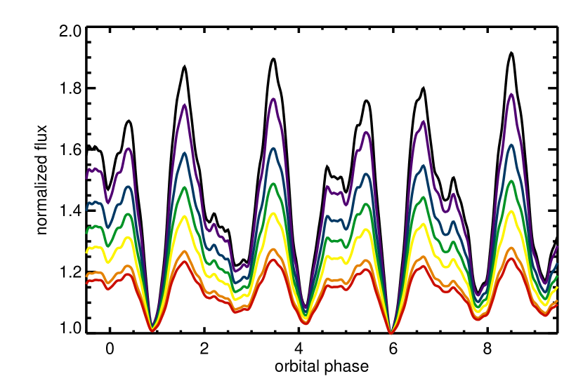
Figure 5: Orbital phase curves as they would be observed in various Spitzer instrumental bands, for the $\eta=0.05$, $\bar{U}=800$ m s^-1 equivalent-barotropic model, assuming simple blackbody emission. From top to bottom the curves are: bolometric (black), 3.6µm (purple), 4.5µm (blue), 6µm (green), 8µm (yellow), 16µm (orange), and 24µm (red). The shorter wavelengths are more variable for the range of temperatures covered by this model. [See the electronic edition of the Journal for a color version of this figure.]

Throughout our discussion so far we have been analyzing bolometric phase curves—i.e., light curves calculated under the simple assumption that the emission from any area on the planetary disk is $\propto T^{4}_{local}$. Here we also compute the light curves that would be measured in each Spitzer instrumental band to determine the wavelength dependence of these model curves. We calculate two values for the flux measured by each Spitzer band: one uses a blackbody for the emitted spectrum from each element area on the planetary disk, and the other one interpolates from a grid of model atmosphere spectra from Seager et al. (2005). This is identical to the procedure adopted in Rauscher et al. (2007a, b). Figure 5 shows the wavelength-dependent phase curves for the $\eta=0.05$, $\bar{U}=800$ m s^-1 simulation, assuming local blackbody emission. The amplitude of variation decreases with increasing wavelength. We have verified that, in the range of temperatures covered by our model runs (see Table 1), this is simply a consequence of the Planck function varying more with temperature at shorter wavelengths than it does at longer wavelengths.

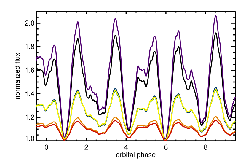
Figure 6: Orbital phase curves as they would be observed in various Spitzer instrumental bands, for the $\eta=0.05$, $\bar{U}=800$ m s^-1 equivalent-barotropic model, using detailed atmospheric spectral models for emission. From top to bottom the curves are: 3.6µm (purple), bolometric (black), followed by overlapping 4.5µm (blue), 6µm (green), and 8µm (yellow), and finally 16µm (orange) and 24µm (red). The results for any given band are strongly affected by the absorption properties of constituents included in the atmospheric spectral model (especially water), but shorter wavelengths are generally more variable for the range of temperatures covered by our circulation model. [See the electronic edition of the Journal for a color version of this figure.]

This same general behavior is seen in Figure 6, in which we plot model phase curves for the same Spitzer bands, but using the detailed spectral models for local emission. Just as with a blackbody, the modeled spectra are more temperature-sensitive at shorter wavelengths. The detailed wavelength-temperature dependence of these spectral models differs from that of a blackbody, however, largely because of the presence of absorption bands, principally those due to water in the atmosphere. Although the presence of water vapor spectral signatures in hot Jupiter atmospheres is currently debated (Barman, 2007; Burrows et al., 2007; Fortney & Marley, 2007; Grillmair et al., 2007; Richardson et al., 2007; Tinetti et al., 2007), the main point of Figures 5 and 6 remains the same: for an atmosphere that spans the range of temperatures expected on hot Jupiters, phase curves at shorter wavelengths may be generally more sensitive to temperature differentials.

One needs to interpret this trend cautiously, however. It is only one of several effects that contribute to the detailed emission properties from such an atmosphere. For example, our modeling strategy based on a vertically-integrated formulation of the atmospheric flow does not capture well the possibility that shorter wavelengths may probe deeper into a planet’s atmosphere (e.g., Seager et al., 2005), where the circulation regime and the horizontal temperature field could in principle differ from higher up. While the model phase curves shown in Figs. 5 and 6 emphasize the role of horizontal temperature variations, additional wavelength-dependent effects are expected from variations of temperature with atmospheric depth. The vertical profile therefore has an effect on the wavelength dependence of phase curves which is unspecified in our models and the behavior shown here can thus only be associated with effect of horizontal temperature variations. Three-dimensional radiation-hydrodynamics models will be required to address this issue reliably.

4 Implications for current and future observations of hot Jupiters

The equivalent-barotropic circulation models of Cho et al. (2003, 2008) indicate the possible existence of large scale weather structures on hot Jupiters. These structures could produce observable signatures in the thermal phase curves of hot Jupiters, in the absence of obscuring elements such as clouds or haze (see, e.g. Pont et al., 2007). We have surveyed the parameter space of these models and find a diverse set of resulting phase curves. This diversity may be relevant in the interpretation of observations from various systems, especially as we are beginning to find that the label “hot Jupiter” may in fact encompass a range of planetary types (e.g., Burrows et al., 2007; Fortney et al., 2007; Hansen & Barman, 2007).

Even within the limited set of observed infrared phase curves, there is already evidence for significant diversity. The first published exoplanet phase curve was a set of five Spitzer 24$\micron$ observations of $\upsilon$ Andromeda b during one of its 4.617-day orbits (Harrington et al., 2006). These authors have found strong variation, indicative of little to no heat redistribution, and a small phase offset consistent with zero. Cowan et al. (2007) used the IRAC instrument on Spitzer to observe HD 209458, HD 179949, and 51 Peg. Their 8$\micron$ data placed an upper limit on the efficiency of heat redistribution on HD 179949b, while both HD 209458b and 51 Peg b were given lower limits. There was no obvious phase shift evident in the data, and these authors chose to fit their data with zero phase-offset models. Hansen et al. (2008) report 24$\micron$ phase curves, with observations at five epochs for $\upsilon$ And, $\tau$ Bootes, and 51 Peg, and at three epochs for the fainter systems HD 179949 and HD 75289. Like for 51 Peg, and in contrast to $\upsilon$ And, there is some evidence for heat redistribution on $\tau$ Boo. Particularly interesting is the detection of an approximately -80^o shift in the phase curve of $\tau$ Boo. This is a phase lag, meaning that the minimum of the curve occurs after transit. Recent MOST photometry of the system indicates that this phase variation may be due to the presence of an active region on the star (Walker et al., 2008). In such a case, it would be more difficult to disentangle the variation in emission due to any longitudinal temperature differences on the planet from additional variations due to the presence of magnetic structures. Nevertheless, the possibility of both positive and negative phase offsets, as found in the phase curves presented here, and as opposed to systematically positive ones according to other dynamical models (e.g., Showman & Guillot, 2002; Cooper & Showman, 2005; Fortney et al., 2006; Langton & Laughlin, 2007) may provide important additional constraints on the regime of circulation present in these atmospheres.

The most detailed observational results published to date are those of Knutson et al. (2007). While the interpretation of other phase observations has been limited by the necessity to fit model curves to a few noisy points spread throughout an orbital period, Knutson et al. (2007) observed HD 189733b continuously for $\sim$33 hours, just over half an orbital period. These authors report an amplitude of variation indicating heat redistribution, although at an incomplete level. The flux maximum occurs 2.3 hours before secondary eclipse, while the minimum is 6.7 hours after transit (=primary eclipse), which corresponds to two separate phase shifts: a +16^o phase shift for the flux maximum, and a $-$47^o shift for the minimum. This means that the data cannot be explained with a simple model that consists solely of a day-night temperature gradient, nor a model whose only atmospheric feature is a hot spot shifted away from the substellar point.

The continuous nature of the Knutson et al. (2007) data allows for the resolution of small features in the phase curve, which was not possible with other published measurements. By postulating a steady emission pattern over the observation time (in the frame rotating with the synchronized planet), these authors reconstruct a longitudinal map of the brightness across the planetary disk. The disk-integrated flux reaches its minimum and maximum values in the same longitudinal hemisphere and a noticeable small scale feature $\sim$20^o wide in phase is seen directly after transit.

Interestingly, we find that similar small scale perturbations can arise in the thermal phase curves of our equivalent-barotropic models. In particular, the $\eta=0.05$, $\bar{U}=800$ m s^-1 model (Figs. 1 and 5) shows such features and produces an overall amplitude of phase curve variations that is qualitatively consistent with the Knutson et al. (2007) data. The min-to-max variation in the data is $\sim$50%, a value consistent with the approximate 20–80% range of single-orbit flux variation seen in this model. Since the features of this model phase curve rely on the presence of large-scale moving atmospheric features, a consequence is that the shape of the phase curve would be expected to vary from one orbit to the next according to our models. This is in fact one of the main qualitative predictions of high-resolution, equivalent-barotropic models for hot Jupiter atmospheres: with strong weather patterns, the temporal variability of the atmospheric temperature field should result in possibly detectable variations for repeated observations of a single system (see also Menou et al., 2003; Rauscher et al., 2007a).

This is particularly relevant in light of the recent 24$\micron$ observation of HD 189733b (Knutson et al., 2008), in which another continuous measurement of the system over a similar half-orbit was performed. Although the circulation regime (e.g., global average wind speeds) could be different in the atmospheric layers probed at 8 and 24$\micron$ (e.g., Seager et al., 2005), the phase curve in Knutson et al. (2008) is similar in amplitude and shape to the 8$\micron$ observation. Thus the global temperature structure seems to have little vertical variation between the two corresponding “photospheres.” Perhaps more importantly, as it pertains to our models, there is little difference in the observed emission pattern between these two orbits. This disfavors any atmospheric model for this planet that predicts significant orbit-to-orbit variations in temperature structure, and specifically the $\eta=0.05$, $\bar{U}=800$ m s^-1 model previously deemed qualitatively consistent with the 8$\micron$ observations. While the small feature seen after transit in the 8$\micron$ data is still indicative of some complexity in the global temperature structure, and the 24$\micron$ data are not of sufficient precision to observe a comparable feature (Knutson et al., 2008), a comparison between these two phase curves points toward a mostly steady global circulation pattern on HD 189733b.

The interpretation of any orbital phase curve data is subtle. Measurements that consist of several discrete observations throughout one orbit may constrain the level of heat redistribution around the planet, but there are degeneracies even with the simplest models when trying to fit the data (Hansen et al., 2008). This type of observation may not easily constrain the level of atmospheric complexity inherent in nonlinear circulation models—even for models as simple as the ones used here. The interpretation of observational data sets like those of Knutson et al. (2007, 2008) becomes ambiguous if variable weather systems are present in hot Jupiter atmospheres, since they can typically vary on orbital timescales. The assumption of a steady atmospheric field (in the planet’s rotating frame) is necessary for the construction of a longitudinal temperature (or brightness) map, so that the resulting inferred properties could become inaccurate if moving features exist.

Repeated observations over multiple orbits help to constrain the steadiness of the global temperature field, as opposed to one which changes from orbit to orbit, like the high $\bar{U}$ models presented here. The permanence of the day side field could also be constrained with repeated secondary eclipse measurements (Rauscher et al., 2007a), which are less observationally expensive than phase curve measurements but lack information on the global day-night pattern. In the future, these two observational techniques should usefully complement each other when applied to eclipsing systems.

Finally, while we have focused our study on thermal phase curves, it is worth noting that the upcoming Kepler mission could potentially also constrain the presence of large-scale weather features in (very) hot Jupiter atmospheres. Indeed, signatures similar to those in thermal phase curves may emerge in reflected light phase curves, if dynamical weather structures such as circumpolar vortices act as distinct thermodynamic regions of the atmospheric flow, with specific cloud and albedo properties. These issues would be best addressed in the future with improved atmospheric circulation models, coupled with radiation transfer calculations.

5 Conclusion

The interpretation of hot Jupiter phase curve data is subtle, especially if variable weather features are present in their atmospheres. We have explored the parameter space of the adiabatic, equivalent-barotropic models of Cho et al. (2003, 2008) to investigate the possible effects that large-scale features would have on hot Jupiter thermal phase curves. Despite their relative simplicity, we find that these models can produce phase curves with shapes that change from one orbit to the next, have apparent phase shifts, and contain small transient perturbations. The detection of such observational signatures would probe the regime of circulation present in these atmospheres. Even the absence of such features would constrain the atmospheric dynamics regime.

We thank the anonymous referee for comments that helped us clarify the manuscript. This work was supported by NASA contract NNG06GF55G.

Table 1: Equivalent-barotropic models under consideration

$\bar{U}$	Min-Max Layer Temperature (K)
(m s-1)	$\eta=0.05$	$\eta=0.10$	$\eta=0.20$
0	1140-1260	1080-1320	960-1440
100	1148-1274	1085-1335	960-1452
200	1113-1284	1081-1338	950-1458
400	998-1313	948-1351	938-1465
800	665-1373	713-1415	722-1504

Figure 1: Bolometric orbital phase curves for equivalent-barotropic model simulations with $\eta=0.05$ and $\bar{U}=$ 800 (dash-dotted), 400 (dotted), 200 (dashed), and 100 (solid) m s^-1. Each curve is normalized to its absolute minimum, emphasizing the relative variation for each model. The phase curves become increasingly complex in models with stronger winds because the temperature field is increasingly dominated by variable weather features. Observable signatures of atmospheric features include small perturbations in the phase curve, offsets in the phase of min./max. flux, and variations in the peak to trough amplitude, from one orbit to the next.

Figure 2: Same as Figure 1 (from top to bottom: $\bar{U}=800,400,200,100$ m s^-1), but for simulations with $\eta=0.10$ (a) and $\eta=0.20$ (b). As the amount of radiative forcing is increased, the imposed day-night temperature contrast becomes the dominant component of the planet’s temperature field, rendering the phase curves more regular in their variation. Nevertheless, large-scale weather features continue to produce deviations away from a strictly regular peak-trough pattern, even for the strong radiative forcing case.

Figure 3: Orbital phase curves for $\bar{U}=800$ m s^-1 equivalent-barotropic models with $\eta=0.05$ (a) and $\eta=0.10$ (b). Three cases, with orbital inclinations $i=$ 90^o (edge-on; dash-dot), 60^o (dotted), and 30^o (solid), are shown in each panel. As the system’s inclination is tilted away from edge-on orientation, the amount of phase variation due to the imposed day-night temperature contrast is decreased, while the signatures of variable weather features become increasingly more apparent in the phase curves. The features that contribute most strongly to the wiggly shapes of these model phase curves are the cold circumpolar vortices, since the change in inclination brings them more into view.

References

- Barman (2007) Barman, T. 2007, ApJ, 661, L191
- Burrows et al. (2007) Burrows, A., Budaj, J., & Hubeny, I. 2007, ArXiv e-prints, arXiv:0709.4080
- Charbonneau et al. (2005) Charbonneau, D., et al. 2005, ApJ, 626, 523
- Cho et al. (2003) Cho, J. Y.-K., Menou, K., Hansen, B. M. S., & Seager, S. 2003, ApJ, 587, L117
- Cho et al. (2008) Cho, J. Y.-K., Menou, K., Hansen, B., & Seager, S. 2008, ApJ accepted, astro-ph/0607338
- Cho & Polvani (1996) Cho, J. Y.-K., & Polvani, L. M. 1996, Physics of Fluids, 8, 1531
- Cooper & Showman (2005) Cooper, C. S., & Showman, A. P. 2005, ApJ, 629, L45
- Cooper & Showman (2006) Cooper, C. S., & Showman, A. P. 2006, ApJ, 649, 1048
- Cowan et al. (2007) Cowan, N. B., Agol, E., & Charbonneau, D. 2007, MNRAS, 552
- Deming et al. (2007a) Deming, D., Agol, E., Charbonneau, D., Cowan, N., Knutson, H., & Marengo, M. 2007, ArXiv e-prints, arXiv:0710.4145
- Deming et al. (2007b) Deming, D., Harrington, J., Laughlin, G., Seager, S., Navarro, S. B., Bowman, W. C., & Horning, K. 2007, ApJ, 667, L199
- Deming et al. (2006) Deming, D., Harrington, J., Seager, S., & Richardson, L. J. 2006, ApJ, 644, 560
- Deming et al. (2005) Deming, D., Seager, S., Richardson, L. J., & Harrington, J. 2005, Nature, 434, 740
- Dobbs-Dixon & Lin (2007) Dobbs-Dixon, I., & Lin, D. N. C. 2007, ArXiv e-prints, arXiv:0704.3269
- Fortney et al. (2006) Fortney, J. J., Cooper, C. S., Showman, A. P., Marley, M. S., & Freedman, R. S. 2006, ApJ, 652, 746
- Fortney et al. (2007) Fortney, J. J., Lodders, K., Marley, M. S., & Freedman, R. S. 2007, ArXiv e-prints, arXiv:0710.2558
- Fortney & Marley (2007) Fortney, J. J., & Marley, M. S. 2007, ApJ, 666, L45
- Grillmair et al. (2007) Grillmair, C. J., Charbonneau, D., Burrows, A., Armus, L., Stauffer, J., Meadows, V., Van Cleve, J., & Levine, D. 2007, ApJ, 658, L115
- Hansen et al. (2008) Hansen, B. et al. 2008, to be submitted to ApJ
- Hansen & Barman (2007) Hansen, B. M. S., & Barman, T. 2007, ArXiv e-prints, arXiv:0706.3052
- Harrington et al. (2006) Harrington, J. et al. 2006, Science, 314, 623
- Harrington et al. (2007) Harrington, J., Luszcz, S., Seager, S., Deming, D., & Richardson, L. J. 2007, Nature, 447, 691
- Knutson et al. (2007) Knutson, H. A., et al. 2007, Nature, 447, 183
- Knutson et al. (2008) Knutson, H. A., et al. 2008, ArXiv e-prints, 802, arXiv:0802.1705
- Langton & Laughlin (2007) Langton, J., & Laughlin, G. 2007, ApJ, 657, L113
- Menou et al. (2003) Menou, K., Cho, J. Y.-K., Seager, S. & Hansen, B. M. S. 2003, ApJ, 587, L113
- Pont et al. (2007) Pont, F., Knutson, H., Gilliland, R. L., Moutou, C. & Charbonneau, D. 2007, MNRAS, in press, arXiv 0712.1374
- Rauscher et al. (2007a) Rauscher, E., Menou, K., Cho, J. Y.-K., Seager, S., & Hansen, B. M. S. 2007a, ApJ, 662, L115
- Rauscher et al. (2007b) Rauscher, E., Menou, K., Seager, S., Deming, D., Cho, J. Y.-K., & Hansen, B. M. S. 2007b, ApJ, 664, 1199
- Redfield et al. (2007) Redfield, S., Endl, M., Cochran, W. D., & Koesterke, L. 2007, ArXiv e-prints, 712, arXiv:0712.0761
- Richardson et al. (2007) Richardson, L. J., Deming, D., Horning, K., Seager, S., & Harrington, J. 2007, Nature, 445, 892
- Salby (1989) Salby, M. L. 1989, Tellus, 41A, 48
- Seager et al. (2005) Seager, S., Richardson, L. J., Hansen, B. M. S., Menou, K., Cho, J. Y.-K., & Deming, D. 2005, ApJ, 632, 1122
- Showman & Guillot (2002) Showman, A. P., & Guillot, T. 2002, A&A, 385, 166
- Showman et al. (2007) Showman, A. P., Menou, K., & Cho, J. Y-K. 2007, ArXiv e-prints, arXiv:0710.2930
- Tinetti et al. (2007) Tinetti, G., et al. 2007, Nature, 448, 169
- Walker et al. (2008) Walker, G. A. H., et al. 2008, ArXiv e-prints, 802, arXiv:0802.2732
- Williams et al. (2006) Williams, P. K. G., Charbonneau, D., Cooper, C. S., Showman, A. P., & Fortney, J. J. 2006, ApJ, 649, 1020