Quadrupole Effect on the Heat Conductivity of Cold Glasses

Abstract

At very low temperatures, the tunneling theory for amorphous solids predicts a thermal conductivity $\kappa\propto T^{p}$, with $p=2$. We have studied the effect of the Nuclear Quadrupole moment on the thermal conductivity of glasses at very low temperatures. We developed a theory that couples the tunneling motion to the nuclear quadrupoles moment in order to evaluate the thermal conductivity. Our result suggests a cross over between two different regimes at the temperature close to the nuclear quadrupoles energy. Below this temperature we have shown that the thermal conductivity is larger than the standard tunneling result and therefore we have $p<2$. However, for temperatures higher than the nuclear quadrupoles energy, the result of standard tunneling model has been found.

I Introduction

Amorphous or glassy materials differ significantly from crystals, especially in the low temperature range. Below $1\rm{K}$, the specific heat $C_{v}$ of dielectric glasses is much larger than in crystalline materials. Moreover, the thermal conductivity $\kappa$ is orders of magnitude lower than the corresponding values found in their crystalline counterparts. $C_{v}$ depends approximately linearly and $\kappa$ almost quadratically on temperatureZel71 . The generally accepted basis to describe the low temperature properties of glasses is the phenomenological tunneling modelPhi72 ; And72 . To explain these behaviors, it was considered that atoms, or groups of atoms, are tunneling between two equilibrium positions, the two minima of a double well potential (DWP). The model is known as the two level system (TLS). In the standard TLS model, these tunneling excitations are considered as independent, and some specific assumptions are made regarding the parameters that characterize themEsq98 .

The TLS can be excited from its ground state to the upper level therefore contributed to the heat capacity. TLSs can also scatter phonons and in this way decrease their mean free path and, correspondingly, the heat conductance.

New interest in this problem was stimulated by several experimental resultsStr98 ; Str00 ; Woh01 ; Nag04 . Until these experiments it was the general believe that the dielectric properties of insulating non-magnetic glasses are independent of external magnetic field. It is very surprising that strong magnetic field effects were discovered in polarization echo experiments at radio frequency and in low frequency dielectric susceptibility measurement at very low temperatures Str98 ; Str00 ; Woh01 . Several generalizations of the standard TLS model have been reported after the anomalous behavior of glasses in a magnetic field. According to these solutions, the models can be divided into ”orbital”Ket99 ; Wue02 ; Lan02 ; Akb05 and ”spin” models (nuclear quadrupole effect)Wue02a ; Wue04 ; Dor03 ; Akb06 . The ”orbital” models can provide an explanation for some of the magnetic field effects by considering the flux dependence of the tunneling splitting. Unfortunately, some assumptions have been made which cannot be reconciled with the standard features of the tunneling model.

A surprising outcome of these experiments is a novel isotope effect observed in different glasses Nag04 . The latter effect shows the important influence of the nuclear quadrupole moments on the observed magnetic field dependence. Therefore it is very important to find the effect of nuclear quadrupole moments on the response function of glasses. For this purpose, in this paper we have studied the thermal properties of heat conductivity of cold glasses taking into account the quadrupole effects. In Section II using Würger’s formalismWue04 , we introduce the nuclear spins in the frame of the two level system model. We will find the general form of the heat conductivity of cold glasses which takes into account the nuclear quadrupole moment in Section III. And finally in section IV, we end this paper by a summery and conclusion on our results.

II TLS coupled by a nuclear spin

The standard TLS can be described as a particle or a small group of particles moving in an effective double-well potential. At very low temperatures only the ground states of each wells are relevant. Using a pseudo-spin representation the Hamiltonian of such a TLS read as

$$H_{TLS}\;=\;\frac{1}{2}\Delta_{0}\sigma_{x}+\frac{1}{2}\Delta\sigma_{z},$$ (1)

where $\Delta$ is the energy off-set at the bottom of the wells, and $\Delta_{0}$ is the tunnel matrix element. Diagonalization of this two state Hamiltonian gives the energies

$$E_{\pm}\;=\;\pm\frac{1}{2}E=\pm\frac{1}{2}\sqrt{\Delta_{0}^{2}+\Delta^{2}}$$

where $E$ is the energy difference between the two wells. According to the randomness of the glassy structure, the energy difference between the two wells have a broad distribution. The energy off-set and the tunneling matrix element are widely distributed and are independent of each other with a uniform distribution of

$${\cal P}\left(\Delta,\Delta_{0}\right)\;=\;\frac{P_{0}}{\Delta_{0}}$$ (2)

where $P_{0}$ is a constant. Using the notations $u=\frac{\Delta_{0}}{E};w=\frac{\Delta}{E}$ which satisfy $u^{2}+w^{2}=1$, the corresponding eigenstates of the diagonal Hamiltonain are given by

$$|\psi_{\pm}\rangle=\sqrt{\frac{1\pm w}{2}}|L\rangle\pm\sqrt{\frac{1\mp w}{2}}|R\rangle$$ (3)

where $|\psi_{-}\rangle$ and $|\psi_{+}\rangle$ are the ground and exited state of the system, respectively. For the moment there is no rigorous theory for tunneling in glasses. It is assumed that atoms or groups of atoms participate in one TLS. As we mentioned before, in the case of the multi-component glasses, one or several of the tunneling atoms carry a nuclear magnetic dipole and an electric quadrupole. When the system moves from one well to another, the atoms change their positions by a fraction of an Ångström.

We can describe the internal motion of the nuclei by a nuclear spin ${\bf I}$ of absolute value ${\bf I}^{2}=\hbar^{2}I(I+1)$. For a nucleus with spin quantum number $I\geq 1$ the charge distribution $\rho({\bf r})$ is not isotropic. Beside the charge monopole, an electric quadrupole moment can be defined with respect to an axis ${\bf e}$

$$Q=\int d^{3}r\left[3({\bf r\cdot e})^{2}-{\bf r}^{2}\right]\rho({\bf r}).$$ (4)

Therefore each level of the pseudo spin projection will split to $(2I+1)$ nuclear spin projections with the quantization axis $m=-I,\ldots,I$.

This can couple to an electric field gradient (EFG) at the nuclear position, expressed by the curvature of the crystal field potential. The potential describing this coupling is written Abr89

$$V_{Q}\;=\;\frac{-eQ}{I(2I-1)}[V_{11}I_{1}^{2}+V_{22}I_{2}^{2}+V_{33}I_{3}^{2}].$$ (5)

The bases used here $(e_{1},e_{2},e_{3})$ are the principal axes of the tensor $V_{ij}$ which describes the electric field gradient, and $e$ is the electron charge. According to the Laplace equation the potential obey $V_{11}+V_{22}+V_{33}=0$. If we define the asymmetry parameter $\eta=\frac{V_{22}-V_{33}}{V_{11}}$, the quadrupole potential can be expressed as:

$$V_{Q}\;=\;\epsilon_{q}[3I_{1}^{2}+\eta(I^{2}_{2}-I_{3}^{2})-I^{2}]$$ (6)

where we denote by $\epsilon_{q}=\frac{-eQV_{11}}{4I(2I-1)}$ the quadrupole coupling constant.

Therefore we can write the quadrupole potential in terms of the reduced two-state coordinate:

$$H_{Q}=\left[V_{Q}^{L}(\frac{1+\sigma_{z}}{2})+V_{Q}^{R}(\frac{1-\sigma_{z}}{2})\right],$$ (7)

where $V_{Q}^{R(L)}$ is defined in Eq. (5) for the particles in right (left) well Dor03 . We can go to basis $|\psi_{\pm}(I,m_{\pm})\rangle=|\psi_{\pm}\rangle\otimes|I,m_{\pm}\rangle$ which have defined as followingWue04

$$H_{\pm}|\psi_{\pm}(I,m_{\pm})\rangle=E_{\pm,m_{\pm}}|\psi_{\pm}(I,m_{\pm})\rangle$$ (8)

where $H_{\pm}=H^{D}_{TLS}+(\frac{V_{Q}^{L}+V_{Q}^{R}}{2})\pm w(\frac{V_{Q}^{L}-V_{Q}^{R}}{2})$ and therefore $E_{\pm,m_{\pm}}=\pm\frac{E}{2}+\epsilon_{m_{\pm}}$; the corresponding eigen-states satisfy:

$$\langle I,m^{\prime}_{\pm}|I,m_{\pm}\rangle=\delta_{m^{\prime}_{\pm},m_{\pm}}$$ (9)

and since $H_{+}$ and $H_{-}$ do not commute, their eigen-states are not generally orthogonal:

$$\langle I,m^{\prime}_{\pm}|I,m_{\mp}\rangle=\chi_{m^{\prime}_{\pm},m_{\mp}}$$ (10)

where these overlaps are dependent on the angle $\theta$. (here $\theta$ is the angle between two axis of the Nuclear quadrupole in each wellsAkb06 : $\widehat{e_{1}^{R},e_{1}^{L}}$)

III Heat Conductivity

The dominant effect of uniform strain field (describing the interaction of the TLS with a phonon field) is on the energy of the tunneling state by changing the asymmetry energy. The changes in the barrier height can usually be ignoredAnd-86 . Any external perturbation is therefore diagonal in the local representation $(|L\rangle,|R\rangle)$ which when transformed into the diagonal representation ( $|\psi_{+}\rangle,|\psi_{-}\rangle$) has the form

$$H_{int}=(\frac{\Delta_{0}}{E}\sigma_{x}+\frac{\Delta}{E}\sigma_{z})\gamma e\cos(\omega t)=H^{\prime}_{int}\cos(\omega t)$$ (11)

in the presence of a strain field $\xi=\xi_{0}\cos(\omega t)$, where $\xi_{0}$ and $\omega$ are the amplitude and the frequency of the strain field respectively. The strain is given by $e=\xi_{0}k_{\alpha}$, and the parameter $\gamma$, defined as $\frac{1}{2}\frac{\partial\Delta}{\partial e}$, is equivalent to elastic dipole moment. Where $k_{\alpha}$ is the phonon wave-vector with polarization $\alpha$. Here the tensorial nature of $e$ has been ignored and $\gamma e$ is written as an average over orientations. Therefore we can easily showphi87 that $e=(\frac{\hbar}{2\rho\omega})^{\frac{1}{2}}k_{\alpha}$, where $\rho$ is the bulk density and $\hbar$ is the Planck constant.

Using Fermi Golden Rule, one can obtain the contribution of a phonon with wave vector $k_{\alpha}$ and polarization $\alpha$ to the generalized TLS transition probability due to phonon emission and absorption, respectively:

$$\Gamma^{em_{\alpha}}_{m^{\prime}_{+}\longrightarrow m_{-}} = \frac{2\pi}{\hbar}\mid\langle\psi_{+}(I,m^{\prime}_{+})\mid H^{\prime}_{int}\mid\psi_{-}(I,m_{-})\rangle\mid^{2}$$

$$\times n_{E_{+,m^{\prime}_{+}}}\delta(E_{+,m^{\prime}_{+}}-E_{-,m_{-}}-\hbar\omega_{\alpha})$$

and

$$\Gamma^{ab_{\alpha}}_{m_{-}\longrightarrow m^{\prime}_{+}} = \frac{2\pi}{\hbar}\mid\langle\psi_{-}(I,m_{-})\mid H^{\prime}_{int}\mid\psi_{+}(I,m^{\prime}_{+})\rangle\mid^{2}$$

$$\times n_{E_{-,m_{-}}}\delta(E_{+,m^{\prime}_{+}}-E_{-,m_{-}}-\hbar\omega_{\alpha})$$

where $n_{E_{\pm,m_{\pm}}}=e^{-\beta E_{\pm,m_{\pm}}}/Z$ is the Boltzmann weight, $Z=\sum_{\pm,m_{\pm}}e^{-\beta E_{\pm,m_{\pm}}}$, $\beta=\frac{1}{K_{B}T}$, $K_{B}$ is the Boltzmann constant and $T$ is temperature. It must be noted here that the transition between the same TLS levels are zero:

$$\langle\psi_{-}(I,m_{\pm})\mid H^{\prime}_{int}\mid\psi_{+}(I,m^{\prime}_{\pm})\rangle=0\longrightarrow\Gamma_{m_{\pm}\longrightarrow m^{\prime}_{\pm}}=0.$$

Therefore the phonon relaxation time can be found by summing $\Gamma^{ab_{\alpha}}_{m_{-}\longrightarrow m_{+}}-\Gamma^{em_{\alpha}}_{m^{\prime}_{+}\longrightarrow m^{\prime}_{-}}$ over all spin states:

$$\tau^{-1}_{\alpha}=\sum_{m_{-},m^{\prime}_{+}} \frac{2\pi\gamma_{\alpha}^{2}\omega_{\alpha}}{\rho v_{\alpha}^{2}}u^{2}|\chi_{m^{\prime}_{+},m_{-}}|^{2}t_{m_{-},m^{\prime}_{+}}(E)$$ (12)

$$\times\delta[E-(\epsilon_{m_{-}}-\epsilon_{m^{\prime}_{+}}+\hbar\omega_{\alpha})],$$

where $v_{\alpha}$ is the sound velocity. Denoting

$$t_{m_{-},m^{\prime}_{+}}(E) = n_{E_{-,m_{-}}}-n_{E_{+,m^{\prime}_{+}}}$$

$$= \frac{e^{\beta E}e^{-\beta\epsilon_{m_{-}}}-e^{-\beta\epsilon_{m^{\prime}_{+}}}}{e^{\beta E}\sum_{m_{-}}e^{-\beta\epsilon_{m_{-}}}+\sum_{m^{\prime}_{+}}e^{-\beta\epsilon_{m^{\prime}_{+}}}}.$$

and after some calculations and averaging over TLS parameters (using Eq. 2), it can be easily shown that

$$\tau^{-1}_{\alpha} = \frac{P_{0}\pi\gamma_{\alpha}^{2}\omega_{\alpha}}{\rho v_{\alpha}^{2}}$$

$$\times \sum_{m_{-},m^{\prime}_{+}}|\chi_{m^{\prime}_{+},m_{-}}|^{2}t_{m_{-},m^{\prime}_{+}}(\epsilon_{m_{-}}-\epsilon_{m^{\prime}_{+}}+\hbar\omega_{\alpha}).$$

Neglecting the phase difference between the nuclear moments in the two wells and assumming that the EFG in both wells are the same $(\chi_{m^{\prime}_{+},m_{-}}=\delta_{m^{\prime}_{+},m_{-}}\Rightarrow\epsilon_{m_{-}}=\epsilon_{m^{\prime}_{+}})$, the famous result of the standard TLS model can be found:

$$\tau^{-1}_{\alpha} = \frac{P_{0}\pi\gamma_{\alpha}^{2}\omega_{\alpha}}{\rho v_{\alpha}^{2}}\tanh(\beta\hbar\omega_{\alpha}).$$ (15)

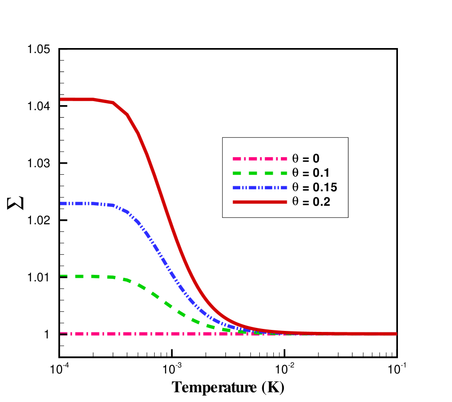
Figure 1: Thermal variation of the ratio parameter $\Sigma$, for $I=1$, $\epsilon_{q}=1\mbox{mK}$ and the different angle between the Nuclear Quadrupole moment in each TLS wells.

The thermal conductivity $\kappa(T)$ is evaluated on the assumption that heat is carried by non-dispersive sound waves, therefore one can write

$$\kappa(T) = \frac{1}{3}\sum_{\alpha}\int_{0}^{\infty}l(\omega_{\alpha})C_{V}(\omega_{\alpha})g(\omega_{\alpha})v_{\alpha}d\omega_{\alpha},$$ (16)

where $l(\omega_{\alpha})=v_{\alpha}/\tau^{-1}_{\alpha}$ is the phonon mean free path of angular frequency $\omega_{\alpha}$, $g(\omega_{\alpha})=\frac{\omega_{\alpha}^{2}}{2\pi^{2}v_{\alpha}^{3}}$ is the phonon frequency distribution function, and $C_{V}(\omega_{\alpha})$ is the heat capacity of phonon which is given by

$$C_{V}(\omega_{\alpha})=\frac{1}{(K_{B}T^{2})}(\frac{\hbar\omega_{\alpha}}{2})^{2}\mathop{{\rm csch}}\!^{2}(\frac{\beta\hbar\omega_{\alpha}}{2}).$$ (17)

By defining $x=\frac{\beta\hbar\omega_{\alpha}}{2}$ and using the above equations the heat conductivity can be obtained,

$$\kappa(T)=\Sigma(T)\times\kappa_{TLS}(T)$$ (18)

where $\kappa_{TLS}(T)=\sum_{\alpha}\frac{\rho v_{\alpha}}{6\pi\hbar^{2}P_{0}\gamma_{\alpha}^{2}}K_{B}^{3}T^{2}$ is the standard TLS (STLS) heat conductivityblack78 , and the coefficient $\Sigma(T)$ is defined by

$$\Sigma(T)=\frac{4}{\pi^{2}}\int_{0}^{\infty}\frac{x^{3}\mathop{{\rm csch}}^{2}(x)dx}{\sum_{m^{\prime}_{+},m_{-}}|\chi_{m^{\prime}_{+},m_{-}}|^{2}t_{m_{-},m^{\prime}_{+}}(\epsilon_{m_{-}}-\epsilon_{m^{\prime}_{+}}+2x/\beta)},$$

(19)

As the exact behavior of the Heat Conductivity can not be found analytically, we are trying to solve Eq. 19 numerically. Assuming that $I=1$ and $\epsilon_{q}=1\mbox{ mK}$ as suggested by echo experiments, we observed the behavior of parameter $\Sigma(T)$ in term of temperature. The results are peresented on Fig. (1) for different values of quadrupole angle ($\theta$) and by averaging over the $\eta$ parameter.

It can be seen that in high temperature regimes $(\epsilon_{q}\ll K_{B}T)$, this ratio $(\Sigma)$ goes to one. As it is predictable where the nuclear part effect can be neglected and heat conductivity behaves as the Standard TLS model. Decreasing temperature this ratio grows and will be saturated at very low temperatures.

In agreement with expectation, at zero quadrupole angle the heat conductivity is the same as the result found from the standard TLS model (please see Eq.III and the statements before that). At low temperature regime, increasing the quadrupole angle with small value cause the heat conductivity saturated value to be larger than what is found form the standard TLS model up to one percent;

The same behavior can be found for $I=3/2$ and $I=2$. Also it can be shown that by changing $\epsilon_{q}$, the growing regime shows a dependency on the quadrupole energy value; it means that by increasing the magnitude of $\epsilon_{q}$, the growing regime will be shifted to higher temperatures. It shows that there is a cross over between two different regimes in the temperature around the quadrupole energy value.

IV Summary and Conclusion

In this paper we have studied the thermal properties of heat conductivity of cold glasses taking into account the quadrupole effects. To describe the interaction of a TLS with nuclear quadrupole, we have used a generalization of the standard TLS Hamiltonian with nuclear spin. The nuclear quadrupole of these systems leads to a splitting of the nuclear spin levels, which is different for the ground state and the excited state. The presence of this multi-level structure causes to increase the heat conductivity magnitude compared to that of simple two-level systems at lower temperature regimes ($K_{B}T\sim\epsilon_{q}$).

It is shown that the heat conductivity has a cross over between two different regimes at the temperature which is close to the nuclear quadrupole energy, $K_{B}T\sim\epsilon_{q}$. It can be observed that there are three different regimes versus temperature.

The first regime deals with high temperature regime: $K_{B}T\gg\epsilon_{q}$ where the known standard tunneling model results have been found. At this regime the effect of quadrupole energy can be neglected in comparison with the TLS energy scale, therefore the nuclear spin splitting is not observable.

The second regime demonstrates the temperature around nuclear quadrupole energy: $K_{B}T\sim\epsilon_{q}$. In this regime, by decreasing the temperature the heat conductivity increases. This is the cross over regime between the standard TLS behavior and the low temperature regime where the nuclear quadrupole effects become important. In this area the nuclear quadrupole energy levels play an important role in the thermal behavior of the system. Decreasing temprature the nuclear quadrupole energy is comparable to thermal fluctuations.

In general these sub-energy level are not the same in both wells of the TLS. Thus their eigen-states are not orthogonal and have the overlap with each other ($|\chi_{m^{\prime}_{+},m_{-}}|^{2}\neq\delta{m^{\prime}_{+},m_{-}}$ and $\epsilon_{m_{+}}\neq\epsilon_{m_{-}}$). This effect causes the mean free path of phonons to increase therefore the thermal conductivity has larger value in comparison with the simple two level system at low temprature regime. This means that where $K_{B}T\sim\epsilon_{q}$, $\Sigma=1+\epsilon(\theta)$ and heat conductivity exponent, $p$, is less than two instead of the $p=2$ which has been found for standard TLS model.

Finally for the third regime the heat conductivity will be saturated at $K_{B}T\ll\epsilon_{q}$.

To obtain a theorytical expression for this effect, one can write $\chi_{m^{\prime}_{+},m_{-}}=\delta_{m^{\prime}_{+},m_{-}}+\varsigma_{m^{\prime}_{+},m_{-}}$ and $\epsilon_{m_{+}}=\epsilon^{o}_{m_{+}}+\gamma_{m_{+}}$ where $\epsilon^{o}_{m_{+}}=\epsilon_{m_{-}}$, and move to the special limitting case where $\varsigma_{m_{+},m_{-}}\ll\beta\gamma_{m_{+}}$, and $\gamma_{m_{+}}\ll\epsilon^{o}_{m_{+}}$. By a little manipulation it can be easily shown that

$$\epsilon(\theta)=C\times(\delta\beta\gamma)^{2}$$ (20)

where $C=\frac{1}{256}\left[48\pi^{2}+\pi^{4}-384\zeta(3)\right]\approx 0.428$ is a numerical constant; $(\delta\beta\gamma)^{2}=\langle\beta^{2}\gamma^{2}\rangle-\langle\beta\gamma\rangle^{2}$, $\langle\beta\gamma\rangle=\sum_{m_{+}}e^{-\beta\epsilon^{o}_{m_{+}}}\beta\gamma_{m_{+}}/\sum_{m_{+}}e^{-\beta\epsilon^{o}_{m_{+}}}$, and $\langle\beta^{2}\gamma^{2}\rangle=\sum_{m_{+}}e^{-\beta\epsilon^{o}_{m_{+}}}\beta^{2}\gamma_{m_{+}}^{2}/\sum_{m_{+}}e^{-\beta\epsilon^{o}_{m_{+}}}$. It shows clearly that by increasing the quadrupole angle the difference of sub-energy in both wells increases which causes the $\Sigma(T)$ value to increase, in agreement with numerical results.

In conclusion we believe that nuclear quadrupoles play an important role in the nature of glasses at low temperatures. In this respect for solving the problem of cold glasses, it is useful to find the effect of nuclear spin on the other response functions. As far as we know there is no experimental result for the heat conductivityPohl02 in the case $K_{B}T\sim\epsilon_{q}$. Therefore it might be a good suggestion for future experiments to approach lower temperatures or use the glasses with larger quadrupole energy.

References

• (1) R. C. Zeller and R. O. Pohl, Phys. Rev. B 4, 2029 (1971).
• (2) W. A. Philips, J. Low. Temp. Phys. 7, 351 (1972).
• (3) P. W. Anderson, B. I. Halperin and C. M. Varma, Philos. Mag. 25, 1 (1972).
• (4) W. A. Phillips, Rep. Prog. Phys. 50, 1657 (1987).
• (5) P. Esquinazi (ed.), Tunneling Systems in Amorphous and Crystalline Solids, Springer Berlin Heidelberg, New York (1998).
• (6) P.Β Strehlow, C.Β Enss, S. Hunklinger, Phys.Β Rev.Β Lett. 80, 5361 (1998).
• (7) P.Β Strehlow et al., Phys.Β Rev.Β Lett. 84, 1938 (2000).
• (8) M.Β Wohlfahrt et al., Europhys.Β Lett. 56, 690 (2001)
• (9) P. Nagel, A. Fleishmann, S. Hunklinger and C. Enss, Phys. Rev. Lett. 92, 245511 (2004).
• (10) S. Kettemann, P. Fulde, and P. Strehlow, Phys. Rev. Lett. 83, 4325 (1999).
• (11) A.Β WΓΌrger, Phys.Β Rev.Β Lett. 88, 077502 (2002).
• (12) A. Langari, Phys. Rev. B 65, 104201 (2002).
• (13) A. Akbari and A. Langari, Phys. Rev. B, 72, 024203 (2005).
• (14) A.Β WΓΌrger, A. Fleischmann, C.Β Enss, Phys.Β Rev.Β Lett. 89, 237601 (2002).
• (15) A. WΓΌrger, J. Low Temp. Phys. 137, 143 (2004).
• (16) D. Bodea and A. WΓΌrger, J. Low Temp. Phys. 136, 39 (2003).
• (17) A. Akbari, D. Bodea, and A. Langari, J. Phys.: Condens. Matter, 19, 466105 (2007).
• (18) A. C. Anderson, Phys. Rev. B, 34, 1317 (1986).
• (19) A. Abragam, The Principles of Nuclear Magnetism, Oxford University Press (1989).
• (20) J. L. Black, Phys.Β Rev.Β B17, 2740 (1978).
• (21) R. O. Pohl, X. Liu, and E. Thompson, Rev. Mod. Phys.74, 991-1013 (2002).