Fluctuation induced quantum interactions between compact objects
and a plane mirror

Abstract

The interaction of compact objects with an infinitely extended mirror plane due to quantum fluctuations of a scalar or electromagnetic field that scatters off the objects is studied. The mirror plane is assumed to obey either Dirichlet or Neumann boundary conditions or to be perfectly reflecting. Using the method of images, we generalize a recently developed approach for compact objects in unbounded space Emig+07b ; Emig+07 to show that the Casimir interaction between the objects and the mirror plane can be accurately obtained over a wide range of separations in terms of charge and current fluctuations of the objects and their images. Our general result for the interaction depends only on the scattering matrices of the compact objects. It applies to scalar fields with arbitrary boundary conditions and to the electromagnetic field coupled to dielectric objects. For the experimentally important electromagnetic Casimir interaction between a perfectly conducting sphere and a plane mirror we present the first results that apply at all separations. We obtain both an asymptotic large distance expansion and the two lowest order correction terms to the proximity force approximation. The asymptotic Casimir-Polder potential for an atom and a mirror is generalized to describe the interaction between a dielectric sphere and a mirror, involving higher order multipole polarizabilities that are important at sub-asymptotic distances.

I Introduction

The interaction between neutral objects is dominated by fluctuation forces due to the coordinated behavior of fluctuating charges or collective modes inside the objects. At zero temperature or at sufficiently small distances, the interactions result from quantum fluctuations. They are important on atomic scales as well as between macroscopic bodies. A prominent example for the latter is the Casimir force between parallel metallic plates due to current or electromagnetic field fluctuations Casimir:1948dh . During the last decade experimental verifications of this effect have been performed with increasing precision. These high precision measurements were enabled by the use of curved surfaces instead of parallel planar mirrors in order to avoid the problem of parallelism. The most commonly employed geometry is a sphere-plate setup that was used in the first high-precision tests of the Casimir effect Lamoreaux+97 ; Mohideen+98 . This geometry has been successfully used ever since in most of the recent experimental studies of Casimir forces between metallic surfaces Roy+99 ; Ederth00 ; Chan+01 ; Chen+02 ; Chen:2006c ; Decca:2007a ; Chen:2007b ; Munday:2007a . In order to keep the deviations from two parallel plates sufficiently small, spheres with a radius much larger than the surface distance have been used. The effect of curvature has been accounted for by the “proximity force approximation” (PFA) Parsegian . This scheme is assumed to describe the interaction for sufficiently small ratios of radius of curvature to distance. However, this an uncontrolled assumption since PFA becomes exact only for infinitesimal separations, and corrections to PFA are generally unknown.

At the other extreme, the interaction between a planar surface and objects that are either very small or at asymptotically large distance is governed by the Casimir-Polder potential that was derived for the case of an atom and a perfectly conducting plane Casimir+48 . This limit has been probed experimentally with high precision for a Bose-Einstein condensate that was trapped close to a planar surface Harber:2005 . Recently, there have been first attempts to go beyond the two extreme limits of asymptotically large and small separations by measuring the Casimir force between a sphere and a plane over a larger range of ratios of sphere radius to distance Krause:2007a .

So far, no theoretical prediction is available that can describe the electromagnetic Casimir interaction between a compact object and a planar surface at all distances, including the important sphere-plate geometry. Until recently, progress in understanding the geometry dependence of fluctuation forces was hampered by the lack of practical methods that are applicable at all separations. Conceptually, the effect of geometry and shape is difficult to study due to the non-additivity of fluctuation forces. Explicit consequences of this non-additivity and also non-monotonic changes in the force have been recently predicted for a pair of cylinders next to planar walls Rodriguez:2007a+b . This behavior has been interpreted in terms of collective charge fluctuations inside the bodies Rahi:2007a .

For some decades, there has been considerable interest in the theory of Casimir forces between objects with curved surfaces. Two types of approaches have been pursued. Attempts to compute the force explicitly in particular geometries and efforts to develop a general framework which yields the interaction in terms of characteristics of the objects like polarizability or curvature. Within the second type of approach, Balian and Duplantier studied the electromagnetic Casimir interaction between compact perfect metals in terms of a multiple reflection expansion and derived also explicit results to leading order at asymptotically large separations Balian . For parallel and partially transmitting plates a connection to scattering theory has been established which yields the Casimir interaction of the plates as a determinant of a diagonal matrix of reflection amplitudes Jaeckel:1991 . For non-planar, deformed plates, a general representation of the Casimir energy as a functional determinant of a matrix that describes reflections at the surfaces and free propagation between them has been developed in Ref. Emig+04 . Later on, an equivalent representation has been applied to perturbative computations in the case of rough and corrugated plates with finite conductivity Neto+05 ; Lambrecht+06 .

Functional determinant formulas have been used also for open geometries that do not fall into the class of parallel plates with deformations. For the electromagnetic Casimir interaction between a planar plate and infinitely long cylinders, a partial wave expansion of the functional determinant has been developed Emig+06 . The same results have been reobtained and used to compute corrections to the PFA for the cylinder-plate geometry in Ref. Bordag06 . Kenneth and Klich identified the inverted Green’s function in the functional determinant as a T-matrix and derived a formal result for the Casimir interaction in terms of this matrix in the case of scalar fields in a medium with a space and frequency dependent speed of light Kenneth+06 .

Recently we described a new method based on a multipole expansion of fluctuating charges that makes possible accurate and efficient calculations of Casimir forces and torques between any number of compact objects Emig+07b ; Emig+07 . The method applies to electromagnetic fields and dielectrics as well as perfect conductors. It also applies to other fields, such as scalar and Dirac, and to any boundary conditions. In this approach, the Casimir energy is given in terms of the fluctuating field’s scattering amplitudes from the individual objects, which encode the effects of the shape and boundary conditions. An equivalent partial wave expansion has been applied to a scalar model for dielectrics Kenneth+07 .

Casimir interactions due to scalar field fluctuations serve as a simplified model for the full electromagnetic interaction. This model is usually easier to analyze and provides an important tool in developing conceptually new approaches and in estimating geometry dependencies. For the sphere-plate geometry with Dirichlet boundary conditions Bulgac et al. obtained the Casimir interaction over a wide range of separations from a modified Krein trace formula Bulgac+06 ; Wirzba:qfext07 . Most notably in the context of scalar fields, a versatile numerical world-line algorithm based on Monte Carlo methods has been developed and applied to a number of interesting geometries, including the here studied sphere-plate interaction Gies+06a ; Gies+06b .

In this work, we extend our approach developed in Refs. Emig+07b ; Emig+07 to describe the interaction of compact objects in the presence of a plane mirror. Our general result holds for scalar and electromagnetic fields. In the electromagnetic case the mirror is assumed to be perfectly conducting but the compact objects can be dielectrics or perfect conductors. The derivation of the general result for the Casimir interaction, see Eqs. (II.48) and (II.100), is given in Section II by combining a functional integral approach and the method of images. In Section III we apply our approach to compute the interaction of a sphere with a plane mirror over a wide range of separations for the scalar Dirichlet and Neumann problem and for the electromagnetic field that is most relevant to applications. We provide a large distance expansion of the interaction, generalizing the Casimir-Polder potential to include higher order multipole polarizabilities. For small separations, we compute the two leading correction terms to the PFA.

II Interaction between fluctuating sources and their images

In this Section we first review the functional integral formulation of Casimir interactions between compact objects for a scalar field and the electromagnetic field. The fluctuating field is integrated out in order to obtain an effective action for the fluctuating sources on the objects. Then we show that the interaction of compact objects with an infinite plane mirror can be described by the equivalent problem of the interaction of compact objects with their mirror images in otherwise empty space, i.e., without the plane mirror. This equivalence holds for Dirichlet or Neumann boundary conditions (at the mirror and the objects) for a scalar field and for a perfectly conducting mirror plane and arbitrary dielectric objects in the case of electromagnetic fluctuations.

II.1 Scalar field

We first consider a real quantum field $\phi({\bf x},t)$ in order to introduce the method of images in the path integral formulation of Casimir interactions. We assume that the space is divided into two half spaces by a mirror plane at $z=0$. $N$ fixed closed surfaces $\Sigma_{\alpha}$, $\alpha=1,\ldots,N$, are located in the right half space ($z>0$). These surfaces are regarded as the boundaries of objects on which either Dirichlet or Neumann boundary conditions are imposed. The action of the unconstrained field in Minkowski space is

$$S[\phi]=\frac{1}{2}\int dt\int_{>}d{\bf x}\left\{\frac{1}{c^{2}}(\partial_{t}\phi)^{2}-(\nabla\phi)^{2}\right\}\,.$$ (II.1)

Here the ${\bf x}$-integration runs over the right half space, indicated by $\int_{>}$. The free energy ${\mathcal{F}}$ of the constraint field $\phi({\bf x},t)$ at inverse temperature $\beta$ is represented by the Euclidean functional integral

$$e^{-\beta{\mathcal{F}}}=Z=\int[{\mathcal{D}}\phi]_{\mathcal{C}}\exp\left(-S_{E}[\phi]/\hbar\right)\,,$$ (II.2)

where the Euclidean action $S_{E}$ follows from Eq. (II.1) after the Wick rotation $ct=-ix^{0}$,

$$S_{E}=\frac{1}{2c}\int_{0}^{\Lambda}dx^{0}\int_{>}d{\bf x}\left\{(\partial_{0}\phi)^{2}+(\nabla\phi)^{2}\right\}$$ (II.3)

with $\Lambda=\beta\hbar c$. The functional integral is over all fields that are periodic in the $x_{0}$-interval from $0$ to $\Lambda$ and that obey the boundary conditions at the surfaces, indicated by the subscript ${\mathcal{C}}$.

The surfaces are fixed and the boundary conditions are time independent. Hence each Fourier component of the field with respect to $x^{0}$ obeys the constraints at the surfaces separately. To make use of this property, we expand $\phi({\bf x},x^{0})$ as

$$\phi({\bf x},x^{0})=\sum_{n=-\infty}^{\infty}\phi_{n}({\bf x})e^{i\kappa_{n}x^{0}}$$ (II.4)

with Matsubara frequencies $\kappa_{n}=2\pi n/\Lambda$ and $\phi_{-n}({\bf x})=\phi^{*}_{n}({\bf x})$. The functional integral splits into independent functional integrals over the $\phi_{n}({\bf x})$ and the logarithm of $Z$ can be written as the sum

$$\ln Z=$$ (II.5)

$$\!\!\!\sum_{n=-\infty}^{\infty}\!\ln\int[{\mathcal{D}}\phi_{n}]_{\mathcal{C}}\exp\left[-\frac{\Lambda}{2\hbar c}\int_{>}\!\!d{\bf x}\left\{\kappa_{n}^{2}|\phi_{n}|^{2}+|\nabla\phi_{n}|^{2}\right\}\right]\,.$$

In the following we are interested in the limit of zero temperature. Then $\Lambda\to\infty$, and the sum over $n$ can be replaced by the integral $\frac{\Lambda}{2\pi}\int_{-\infty}^{\infty}d\kappa$ and $\phi_{n}({\bf x})$ is replaced by $\phi({\bf x},\kappa)$. Combining positive and negative $\kappa$, we get

$$\ln Z=\frac{\Lambda}{2\pi}\int_{0}^{\infty}d\kappa\ln\mathcal{Z}(\kappa)$$ (II.6)

with

$$\mathcal{Z}(\kappa)\!=\!\int[{\mathcal{D}}\phi({\bf x},\kappa)]_{\mathcal{C}}[{\mathcal{D}}\phi^{*}({\bf x},\kappa)]_{\mathcal{C}}\exp\left[-\frac{\Lambda}{\hbar c}\int_{>}\!\!d{\bf x}\left\{\kappa^{2}|\phi|^{2}+|\nabla\phi|^{2}\right\}\right]\,.$$ (II.7)

The ground state energy is obtained from $Z$ as

$${\cal E}_{0} = -\lim_{\beta\to\infty}\frac{1}{\beta}\ln Z$$ (II.8)

$$= -\frac{\hbar c}{2\pi}\int_{0}^{\infty}d\kappa\ln\mathcal{Z}(\kappa)\,.$$

The Casimir energy is the difference between the ground state energy of the surfaces at their actual distance and the sum of the ground state energies of the separate surfaces which is obtained by removing the surfaces to infinite separation,

$${\cal E}=-\frac{\hbar c}{2\pi}\int_{0}^{\infty}d\kappa\ln\frac{\mathcal{Z}(\kappa)}{\mathcal{Z}_{\infty}(\kappa)}\,,$$ (II.9)

where $\mathcal{Z}_{\infty}(\kappa)$ is the partition function for the surfaces with infinite separation. In the following we suppress the label $\kappa$. Next, the constraints at the objects are implemented by functional $\delta$-functions Bordag+85 ; LK91 . For Dirichlet boundary conditions, $\phi=0$, on the surfaces $\Sigma_{\alpha}$, the constraint functional integral can be expressed in terms of an unconstrained integral by using

$$\int[{\mathcal{D}}\phi]_{\mathcal{C}}[{\mathcal{D}}\phi^{*}]_{\mathcal{C}}=$$ (II.10)

$$\!\!\!\!\!\int\!\!{\mathcal{D}}\phi{\mathcal{D}}\phi^{*}\prod_{\alpha=1}^{N}\int\!\!{\mathcal{D}}\varrho_{\alpha}{\mathcal{D}}\varrho^{*}_{\alpha}\exp\left[i\!\!\int_{\Sigma_{\alpha}}\!\!\!\!\!d{\bf x}\,\left\{\varrho_{\alpha}^{*}({\bf x})\phi({\bf x})+{\mbox{c.c.\,}}\right\}\right],$$

where the $\delta$-functions at each position of the surfaces have been written as an integral over a source field $\varrho_{\alpha}({\bf x})$ that is non-zero on the surfaces $\Sigma_{\alpha}$ only. When we use this representation of the constraints in Eq. (II.7), the now unconstrained functional integral over $\phi({\bf x})$ is Gaussian and yields

$$\mathcal{Z}(\kappa) = \mathcal{Z}_{0}\prod_{\alpha=1}^{N}\int{\mathcal{D}}\varrho_{\alpha}{\mathcal{D}}\varrho^{*}_{\alpha}\exp\left[-\frac{\hbar c}{2\Lambda}\sum_{\alpha\beta}\int_{\Sigma_{\alpha}}\!\!d{\bf x}\int_{\Sigma_{\beta}}\!\!d{\bf x}^{\prime}\left\{\varrho^{*}_{\alpha}({\bf x})G_{>}({\bf x},{\bf x}^{\prime},\kappa)\varrho_{\beta}({\bf x}^{\prime})+{\mbox{c.c.\,}}\right\}\right]$$ (II.11)

$$\equiv \mathcal{Z}_{0}\prod_{\alpha=1}^{N}\int{\mathcal{D}}\varrho_{\alpha}{\mathcal{D}}\varrho^{*}_{\alpha}e^{-(\hbar c/\Lambda)\tilde{S}[\varrho]}\,,$$

where $\mathcal{Z}_{0}$ is the partition function of the field in the right half space without the surfaces $\Sigma_{\alpha}$. For Neumann boundary conditions at the surfaces $\Sigma_{\alpha}$ the field $\phi({\bf x})$ in the exponential of Eq. (II.10) is replaced by $\partial_{n}\phi({\bf x})$ and $G_{>}({\bf x},{\bf x}^{\prime},\kappa)$ in Eq. (II.11) is replaced by $\partial_{n}\partial_{n^{\prime}}G_{>}({\bf x},{\bf x}^{\prime},\kappa)$, where $\partial_{n}$ is the normal derivative pointing out of the objects. Here $G_{>}({\bf x},{\bf x}^{\prime},\kappa)$ is the free Green’s function in the right half space which is given by

$$G_{>}({\bf x},{\bf x}^{\prime},\kappa)=G_{0}({\bf x},{\bf x}^{\prime},\kappa)\mp G_{0}({\bf x},{\bf x}_{R}^{\prime},\kappa)\,,$$ (II.12)

where ${\bf x}_{R}=({\bf x}_{\|},-z)$ is the mirror image of ${\bf x}=({\bf x}_{\|},z)$ and the $-$($+$) sign applies to Dirichlet (Neumann) boundary conditions at the mirror plane at $z=0$. The Green’s function of free unbounded space is given by

$$G_{0}({\bf x},{\bf x}^{\prime},\kappa)=\frac{e^{ik|{\bf x}-{\bf x}^{\prime}|}}{4\pi|{\bf x}-{\bf x}^{\prime}|}_{|k\to i\kappa}\,.$$ (II.13)

Using Eq. (II.12) the action $\tilde{S}[\varrho]$ defined by Eq. (II.11) can be expressed in terms of the original sources $\varrho_{\alpha}({\bf x})$ and their mirror sources $\varrho^{R}_{\alpha}({\bf x})$,

$$\tilde{S}[\varrho]=\frac{1}{2}\sum_{\alpha\beta}\left\{\int_{\Sigma_{\alpha}}d{\bf x}\int_{\Sigma_{\beta}}d{\bf x}^{\prime}\varrho^{*}_{\alpha}({\bf x})G_{0}({\bf x},{\bf x}^{\prime},\kappa)\varrho_{\beta}({\bf x}^{\prime})\right.$$ (II.14)

$$+ \!\!\!\left.\int_{\Sigma_{\alpha}}d{\bf x}\int_{\Sigma^{R}_{\beta}}d{\bf x}^{\prime}\varrho^{*}_{\alpha}({\bf x})G_{0}({\bf x},{\bf x}^{\prime},\kappa)\varrho^{R}_{\beta}({\bf x}^{\prime})+{\mbox{c.c.\,}}\right\}$$

for Dirichlet boundary conditions at the surfaces $\Sigma_{\alpha}$ and with $G_{0}({\bf x},{\bf x}^{\prime},\kappa)$ replaced by $\partial_{n}\partial_{n^{\prime}}G_{0}({\bf x},{\bf x}^{\prime},\kappa)$ for Neumann boundary conditions at the surfaces $\Sigma_{\alpha}$. Here we have introduced the mirror sources

$$\varrho_{\alpha}^{R}({\bf x})=\mp\varrho_{\alpha}({\bf x}_{R})\,,$$ (II.15)

where the $-$ ($+$) sign applies to a Dirichlet (Neumann) mirror. The mirror sources are located on the mirror surfaces $\Sigma_{\alpha}^{R}$ that are obtained from the $\Sigma_{\alpha}$ by $z\to-z$ for all surface positions, see Fig. 1. The first term of the action of Eq. (II.14) describes the interaction of the surface sources in the absence of the mirror plane. The second term couples each surface source to all mirror sources. Since the mirror problem is now described by an action in free space with sources and mirror sources, we can apply the concepts of the previously developed approach for Casimir interactions between compact objects in unbounded space Emig+07 . Below, we provide an explicit derivation for the case of Dirichlet boundary conditions at the surfaces $\Sigma_{\alpha}$ but we shall also indicate how the derivation has to be modified for Neumann boundary conditions.

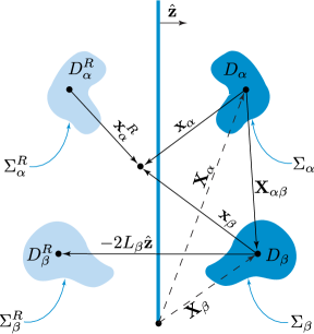
Figure 1: Geometry with original surfaces $\Sigma_{\alpha}$ (objects $D_{\alpha}$) in the right half space ($z>0$) and mirror surfaces $\Sigma_{\alpha}^{R}$ (objects $D_{\alpha}^{R}$). ${\bf x}_{\alpha}$, ${\bf x}_{\alpha}^{R}$ are local coordinate vectors measured from the object’s origins, $L_{\beta}$ is the center-to-mirror distance of surface $\Sigma_{\beta}$ (object $D_{\beta}$).

The action of Eq. (II.14) is composed of two qualitatively different terms that we will now consider separately. Firstly, there are terms that couple sources on different surfaces (${\bf x}\neq{\bf x}^{\prime}$) where we use the term “surface” in the following for the original and the mirror surfaces. We shall call these terms off-diagonal. As diagonal terms we shall denote those which couple sources on the same surface (${\bf x}={\bf x}^{\prime}$ possible). Both type of terms can be expressed in terms of the multipole moments of the sources.

Off-diagonal terms — These terms couple sources on different objects,

$$\tilde{S}_{\alpha\beta}=\frac{1}{2}\int_{\Sigma_{\alpha}}d{\bf x}_{\alpha}\left\{\varrho^{*}_{\alpha}({\bf x}_{\alpha})\phi_{\beta}({\bf x}_{\alpha})+{\mbox{c.c.\,}}\right\}$$ (II.16)

for $\alpha\neq\beta$ and the original sources to the mirror sources,

$$\tilde{S}^{R}_{\alpha\beta}=\frac{1}{2}\int_{\Sigma_{\alpha}}d{\bf x}_{\alpha}\left\{\varrho^{*}_{\alpha}({\bf x}_{\alpha})\phi^{R}_{\beta}({\bf x}_{\alpha})+{\mbox{c.c.\,}}\right\}$$ (II.17)

for all $\alpha$, $\beta$. Here we have introduced local coordinates ${\bf x}_{\alpha}$ that are measured relative to an arbitrarily chosen origin that is located inside the surface $\alpha$, see Fig. 1. We have also defined the fields

$$\phi_{\beta}({\bf x}) = \int_{\Sigma_{\beta}}d{\bf x}^{\prime}G_{0}({\bf x},{\bf x}^{\prime},\kappa)\varrho_{\beta}({\bf x}^{\prime})$$

$$\phi^{R}_{\beta}({\bf x}) = \int_{\Sigma^{R}_{\beta}}d{\bf x}^{\prime}G_{0}({\bf x},{\bf x}^{\prime},\kappa)\varrho^{R}_{\beta}({\bf x}^{\prime})\,,$$ (II.18)

which are the classical fields generated by the sources. For Neumann boundary conditions on the surfaces $\Sigma_{\alpha}$, $\phi_{\beta}({\bf x}_{\alpha})$ and $\phi^{R}_{\beta}({\bf x}_{\alpha})$ in Eqs. (II.16) and (II.17) have to be replaced by $\partial_{n}\phi_{\beta}({\bf x}_{\alpha})$ and $\partial_{n}\phi^{R}_{\beta}({\bf x}_{\alpha})$, respectively. Also, $G_{0}({\bf x},{\bf x}^{\prime},\kappa)$ in Eq. (II.1) has to be replaced by $\partial_{n^{\prime}}G_{0}({\bf x},{\bf x}^{\prime},\kappa)$.

Since we can assume that every position on $\Sigma_{\alpha}$ is outside a sphere enclosing $\Sigma_{\beta}$ or $\Sigma^{R}_{\beta}$, we can use the partial wave expansion of $G_{0}({\bf x},{\bf x}^{\prime},\kappa)$ for $|{\bf x}^{\prime}|<|{\bf x}|$,

$$G_{0}({\bf x},{\bf x}^{\prime},\kappa)=-\kappa\sum_{lm}j_{l}(i\kappa r^{\prime})h_{l}^{(1)}(i\kappa r)Y_{lm}(\hat{\bf x})Y_{lm}^{*}(\hat{\bf x}^{\prime})\,.$$ (II.19)

When we consider Eq. (II.1) with coordinates ${\bf x}_{\beta}$ relative to the origin inside surface $\Sigma_{\beta}$, the field that is generated by the source $\varrho_{\beta}$ can be written as

$$\phi_{\beta}({\bf x}_{\beta})=-\kappa\sum_{lm}Q_{\beta,lm}h_{l}^{(1)}(i\kappa r_{\beta})Y_{lm}(\hat{\bf x}_{\beta})\,,$$ (II.20)

where we have defined the multipole moments of the source $\varrho_{\beta}$ as

$$Q_{\beta,lm}=\int_{\Sigma_{\beta}}d{\bf x}_{\beta}j_{l}(i\kappa r_{\beta})Y_{lm}^{*}(\hat{\bf x}_{\beta})\varrho_{\beta}({\bf x}_{\beta})\,.$$ (II.21)

The field of the mirror sources can be expressed in the same form,

$$\phi^{R}_{\beta}({\bf x}^{R}_{\beta})=-\kappa\sum_{lm}Q^{R}_{\beta,lm}h_{l}^{(1)}(i\kappa r^{R}_{\beta})Y_{lm}(\hat{\bf x}^{R}_{\beta})\,,$$ (II.22)

where ${\bf x}^{R}_{\beta}$ denotes the local coordinates that are measured relative to the origin inside surface $\Sigma_{\beta}^{R}$. The multipole moments of the mirror source are given by

$$Q_{\beta,lm}^{R}=\mp(-1)^{l+m}Q_{\beta,lm}$$ (II.23)

due to Eq. (II.15) and $Y_{lm}(\hat{\bf x}_{R})=(-1)^{l+m}Y_{lm}(\hat{\bf x})$. For Neumann boundary conditions at the surfaces $\Sigma_{\alpha}$ the above expressions remain valid if the multipole moments $Q_{\beta,lm}$ are replaced by Neumann multipoles which have the form of Eq. (II.21) but with $j_{l}(i\kappa r_{\beta})Y_{lm}^{*}(\hat{\bf x}_{\beta})$ replaced by $\partial_{n}[j_{l}(i\kappa r_{\beta})Y_{lm}^{*}(\hat{\bf x}_{\beta})]$.

In order to express the action of Eq. (II.16) in terms of multipole moments, we have to write the field generated by the surface source $\varrho_{\beta}$ as a function of the local coordinate ${\bf x}_{\alpha}$ that is regular at the origin inside $\Sigma_{\alpha}$. This can be done using translation matrices ${\mathbb{U}}$ which relate outgoing ($h_{l}^{(1)}$) and regular ($j_{l}$) spherical Bessel functions,

$$h^{(1)}_{l}(i\kappa r_{\beta})Y_{lm}(\hat{\bf x}_{\beta})=\sum_{l^{\prime}m^{\prime}}\mathcal{U}_{l^{\prime}m^{\prime}lm}({\bf X}_{\alpha\beta})j_{l^{\prime}}(i\kappa r_{\alpha})Y_{l^{\prime}m^{\prime}}(\hat{\bf x}_{\alpha})\,.$$ (II.24)

The matrix elements $\mathcal{U}_{l^{\prime}m^{\prime}lm}$ of ${\mathbb{U}}$ depend on the vector ${\bf X}_{\alpha\beta}={\bf X}_{\beta}-{\bf X}_{\alpha}={\bf x}_{\alpha}-{\bf x}_{\beta}$ from the origin inside $\Sigma_{\alpha}$ to the origin inside $\Sigma_{\beta}$, see Fig. 1, and are given by Emig+07

$$\mathcal{U}_{l^{\prime}m^{\prime}lm}({\bf X}_{\alpha\beta}) = \sqrt{4\pi}(-1)^{m}i^{l-l^{\prime}}\sqrt{(2l+1)(2l^{\prime}+1)}$$ (II.25)

$$\times \sum_{l^{\prime\prime}}i^{l^{\prime\prime}}\sqrt{2l^{\prime\prime}+1}\begin{pmatrix}l&l^{\prime}&l^{\prime\prime}\\ 0&0&0\end{pmatrix}\begin{pmatrix}l&l^{\prime}&l^{\prime\prime}\\ m&-m^{\prime}&m^{\prime}-m\end{pmatrix}h_{l^{\prime\prime}}^{(1)}(i\kappa|{\bf X}_{\alpha\beta}|)Y_{l^{\prime\prime}m-m^{\prime}}(\hat{\bf X}_{\alpha\beta})\,,$$

where we have assumed that the Cartesian coordinate frames associated with the two origins have identical orientation, i.e., they are related by a translation. The summation over $l^{\prime\prime}$ involves only a finite number of terms since the 3-$j$ symbols vanish for $l^{\prime\prime}>l+l^{\prime}$ and $l^{\prime\prime}<|l-l^{\prime}|$.

Using the translation formula of Eq. (II.24), the field generated by the source on surface $\Sigma_{\beta}$, given by Eq. (II.20), can be written as function of the coordinate ${\bf x}_{\alpha}$ as

$$\phi_{\beta}({\bf x}_{\alpha})=-\kappa\sum_{lm}Q_{\beta,lm}\sum_{l^{\prime}m^{\prime}}\mathcal{U}_{l^{\prime}m^{\prime}lm}^{\alpha\beta}j_{l^{\prime}}(i\kappa r_{\alpha})Y_{l^{\prime}m^{\prime}}(\hat{\bf x}_{\alpha})\,,$$ (II.26)

where we have introduced $\mathcal{U}_{l^{\prime}m^{\prime}lm}^{\alpha\beta}\equiv\mathcal{U}_{l^{\prime}m^{\prime}lm}({\bf X}_{\alpha\beta})$. Similarly we obtain for the field generated by the mirror sources of Eq. (II.22), now expressed as function of ${\bf x}_{\alpha}$,

$$\phi^{R}_{\beta}({\bf x}_{\alpha})=\pm\kappa\sum_{lm}Q_{\beta,lm}\sum_{l^{\prime}m^{\prime}}\mathcal{U}_{l^{\prime}m^{\prime}lm}^{R,\alpha\beta}j_{l^{\prime}}(i\kappa r_{\alpha})Y_{l^{\prime}m^{\prime}}(\hat{\bf x}_{\alpha})\,,$$ (II.27)

where we defined

$$\mathcal{U}_{l^{\prime}m^{\prime}lm}^{R,\alpha\beta}\equiv(-1)^{l+m}\mathcal{U}_{l^{\prime}m^{\prime}lm}({\bf x}_{\alpha}-{\bf x}^{R}_{\beta})\,,$$ (II.28)

and used Eq. (II.23). Notice that the latter formula applies also to the case $\alpha=\beta$ which describes the translation between the surface $\Sigma_{\alpha}$ and its mirror image so that the argument of the translation matrix becomes ${\bf x}_{\alpha}-{\bf x}_{\alpha}^{R}=-2L_{\alpha}\hat{\bf z}$ where $L_{\alpha}$ is the normal distance between the origin of surface $\Sigma_{\alpha}$ and the mirror plane. For this case of translations along the $\hat{\bf z}$-direction the translation matrix simplifies to Emig+07

$$\mathcal{U}_{l^{\prime}m^{\prime}lm}(-2L_{\alpha}\hat{\bf z})=\delta_{m^{\prime}m}(-1)^{m}i^{l-l^{\prime}}\sqrt{(2l+1)(2l^{\prime}+1)}\sum_{l^{\prime\prime}}i^{-l^{\prime\prime}}(2l^{\prime\prime}+1)\begin{pmatrix}l&l^{\prime}&l^{\prime\prime}\\ 0&0&0\end{pmatrix}\begin{pmatrix}l&l^{\prime}&l^{\prime\prime}\\ m&-m&0\end{pmatrix}h_{l^{\prime\prime}}^{(1)}(i\kappa 2L_{\alpha})\,.$$ (II.29)

When we substitute the result for the fields of Eqs. (II.26), (II.27) into Eqs. (II.16), (II.17), we obtain the action in terms of the original multipole moments,

$$\sum_{\alpha\neq\beta}\tilde{S}_{\alpha\beta} = -\kappa\sum_{\alpha\neq\beta}\sum_{lml^{\prime}m^{\prime}}Q^{*}_{\alpha,l^{\prime}m^{\prime}}\,\,\tilde{\mathcal{U}}^{\alpha\beta}_{l^{\prime}m^{\prime}lm}\,Q_{\beta,lm}$$

$$\sum_{\alpha\beta}\tilde{S}^{R}_{\alpha\beta} = \pm\kappa\sum_{\alpha\beta}\sum_{lml^{\prime}m^{\prime}}Q^{*}_{\alpha,l^{\prime}m^{\prime}}\,\,\tilde{\mathcal{U}}^{R,\alpha\beta}_{l^{\prime}m^{\prime}lm}\,Q_{\beta,lm}\,,$$

which applies to Dirichlet as well as Neumann boundary conditions at the surfaces $\Sigma_{\alpha}$. To simplify notation, we have defined the modified translation matrix elements

$$\tilde{\mathcal{U}}^{\alpha\beta}_{l^{\prime}m^{\prime}lm} \equiv (-1)^{l^{\prime}}\mathcal{U}^{\alpha\beta}_{l^{\prime}m^{\prime}lm}$$ (II.32)

$$\tilde{\mathcal{U}}^{R,\alpha\alpha}_{l^{\prime}mlm} \equiv (-1)^{l^{\prime}}\mathcal{U}^{R,\alpha\alpha}_{l^{\prime}mlm}$$ (II.33)

$$\tilde{\mathcal{U}}^{R,\alpha\beta}_{l^{\prime}m^{\prime}lm} \equiv \frac{1}{2}\left[(-1)^{l^{\prime}}\mathcal{U}^{R,\alpha\beta}_{l^{\prime}m^{\prime}lm}+(-1)^{l}\mathcal{U}^{{R,\beta\alpha}^{*}}_{lml^{\prime}m^{\prime}}\right],\,(\alpha\neq\beta)$$

Here we have used the definition of Eq. (II.21) and $[j_{l}(i\kappa r)]^{*}=(-1)^{l}j_{l}(i\kappa r)$. In addition, we applied the symmetry relations $\mathcal{U}^{{\alpha\beta}^{*}}_{lml^{\prime}m^{\prime}}=(-1)^{l+l^{\prime}}\mathcal{U}^{\beta\alpha}_{l^{\prime}m^{\prime}lm}$ and $\mathcal{U}^{{R,\alpha\alpha}^{*}}_{lml^{\prime}m}=(-1)^{l+l^{\prime}}\mathcal{U}^{R,\alpha\alpha}_{l^{\prime}mlm}$ which follow from Eqs. (II.25), (II.29), symmetry properties of 3-j symbols and spherical harmonics, and $h_{l}^{(1)}(iz)=-i^{-l}\sqrt{2/(\pi z)}K_{l+1/2}(z)$ where $K_{l+1/2}(z)$ is the (real valued) modified Bessel function of second kind. Notice that the actions of Eqs. (LABEL:eq:S-off-diag-of-Qs), (LABEL:eq:S-off-diag-of-Qs-R) couple sources on different surfaces and hide the dependence on the particular boundary conditions and shape of the surfaces.

Diagonal terms — These are the self-action terms

$$\tilde{S}_{\alpha}=\frac{1}{2}\int_{\Sigma_{\alpha}}d{\bf x}\left\{\varrho^{*}_{\alpha}({\bf x})\phi_{\alpha}({\bf x})+{\mbox{c.c.\,}}\right\}$$ (II.35)

in Eq. (II.14), which we have expressed here in terms of the classical field defined in Eq. (II.1). For Neumann boundary conditions on the surface $\Sigma_{\alpha}$ we have to replace again $\phi_{\alpha}({\bf x})$ by $\partial_{n}\phi_{\alpha}({\bf x})$ in Eq. (II.35). Here and in the following we only use the coordinate system associated with the origin inside $\Sigma_{\alpha}$, and hence drop the label $\alpha$ on the coordinates. The classical field generated by the source $\varrho_{\alpha}({\bf x})$ on surface $\Sigma_{\alpha}$ obeys the Helmholtz equation

$$(\nabla^{2}-\kappa^{2})\phi_{\alpha}({\bf x})=-\varrho_{\alpha}({\bf x})\,.$$ (II.36)

For positions ${\bf x}$ that are located on the surface $\Sigma_{\alpha}$ the total field $\phi({\bf x})$ generated by all sources must obey the same Helmholtz equation. The part of the total field that is generated by sources other than $\varrho_{\alpha}({\bf x})$ can be regarded as incident field $\phi_{0,\alpha}({\bf x})$ at the surface $\Sigma_{\alpha}$, which obeys in region around $\Sigma_{\alpha}$, that is free of sources other than $\varrho_{\alpha}({\bf x})$, the homogeneous Helmholtz equation. Hence the total field can be written as

$$\phi({\bf x}) = \phi_{0,\alpha}({\bf x})+\phi_{\alpha}({\bf x})$$

$$= \phi_{0,\alpha}({\bf x})+\int_{\Sigma_{\alpha}}d{\bf x}^{\prime}\,G_{0}({\bf x},{\bf x}^{\prime},\kappa)\varrho_{\alpha}({\bf x}^{\prime})$$

for all ${\bf x}$ located on $\Sigma_{\alpha}$. For Neumann boundary conditions at $\Sigma_{\alpha}$ the Green’s function in Eq. (II.1) is replaced again by $\partial_{n^{\prime}}G_{0}({\bf x},{\bf x}^{\prime},\kappa)$. We would like to evaluate the action of Eq. (II.35) in terms of multipole moments. Hence, we must consider field configurations with a fixed source on surface $\Sigma_{\alpha}$ that is characterized by its multipole moments. This implies that we have to find the incident field $\phi_{0,\alpha}({\bf x})$ that induces a prescribed set of multipoles $Q_{\alpha,lm}$ on $\Sigma_{\alpha}$. The multipole moments can be identified as the amplitudes of the scattered field which is given by $\phi_{\alpha}({\bf x})$ with ${\bf x}$ located outside of the surface $\Sigma_{\alpha}$. Using the partial wave expansion of Eq. (II.19), we get

$$\phi_{\alpha}({\bf x})=-\kappa\sum_{l^{\prime}m^{\prime}}Q_{\alpha,l^{\prime}m^{\prime}}h_{l^{\prime}}^{(1)}(i\kappa r)Y_{l^{\prime}m^{\prime}}(\hat{\bf x})\,.$$ (II.38)

From scattering theory we know that the amplitudes of the scattered field are related to the amplitudes of the regular incident field by the transition matrix ${\mathbb{T}}$ which is related to the scattering matrix ${\mathbb{S}}$ by ${\mathbb{T}}=({\mathbb{S}}-1)/2$. If we expand the incident field as

$$\phi_{0,\alpha}({\bf x})=\sum_{lm}\phi_{0,\alpha,lm}\,j_{l}(i\kappa r)Y_{lm}(\hat{\bf x})\,,$$ (II.39)

the amplitudes of the scattered field are given by

$$-\kappa Q_{\alpha,l^{\prime}m^{\prime}}=\sum_{lm}{\mathcal{T}}^{\alpha}_{l^{\prime}m^{\prime}lm}\,\phi_{0,\alpha,lm}\,,$$ (II.40)

where the ${\mathcal{T}}^{\alpha}_{l^{\prime}m^{\prime}lm}$ denote the matrix elements of the ${\mathbb{T}}$-matrix of the surface $\Sigma_{\alpha}$. Hence, the amplitudes of the incident field have to be given by

$$\phi_{0,\alpha,lm}=-\kappa\sum_{l^{\prime}m^{\prime}}[{\mathcal{T}}^{\alpha}]^{-1}_{lml^{\prime}m^{\prime}}Q_{\alpha,l^{\prime}m^{\prime}}\,.$$ (II.41)

For Dirichlet boundary conditions, the total field $\phi({\bf x})$ of Eq. (II.1) has to vanish on $\Sigma_{\alpha}$ so that $\phi_{\alpha}({\bf x})=-\phi_{0,\alpha}({\bf x})$ on the surface. Hence, using Eqs. (II.39) and (II.41), the action of Eq. (II.35) can be expressed in terms of the multipole moments of $\varrho_{\alpha}({\bf x})$,

$$\tilde{S}_{\alpha}=\kappa\sum_{lml^{\prime}m^{\prime}}Q^{*}_{\alpha,lm}\,[\tilde{\mathcal{T}}^{\alpha}]^{-1}_{lml^{\prime}m^{\prime}}\,Q_{\alpha,l^{\prime}m^{\prime}}$$ (II.42)

with the modified $\tilde{\mathbb{T}}$-matrix defined by

$$\tilde{\mathcal{T}}^{\alpha}_{l^{\prime}m^{\prime}lm}\equiv(-1)^{l}{\mathcal{T}}^{\alpha}_{l^{\prime}m^{\prime}lm}\,.$$ (II.43)

Here we have used the definition of the multipoles in Eq. (II.21) to integrate over the surface and applied the relation ${\mathcal{T}}^{\alpha^{*}}_{l^{\prime}m^{\prime}lm}=(-1)^{l+l^{\prime}}{\mathcal{T}}^{\alpha}_{lml^{\prime}m^{\prime}}$.

For Neumann boundary conditions on $\Sigma_{\alpha}$, the normal derivative of the total field of Eq. (II.1) has to vanish on $\Sigma_{\alpha}$ so that $\partial_{n}\phi_{\alpha}({\bf x})=-\partial_{n}\phi_{0,\alpha}({\bf x})$ on the surface. When we use the definition of the multipole moments for Neumann boundary conditions, we obtain again Eq. (II.42) but with the matrix ${\mathbb{T}}^{\alpha}$ for Neumann boundary conditions.

Now we can combine all results for off-diagonal and diagonal terms and express the total action of Eq. (II.14) in terms of the original multipole moments. Since we have

$$\tilde{S}=\sum_{\alpha\neq\beta}\tilde{S}_{\alpha\beta}+\sum_{\alpha}\tilde{S}_{\alpha}+\sum_{\alpha,\beta}\tilde{S}^{R}_{\alpha\beta}$$ (II.44)

we obtain from Eqs. (LABEL:eq:S-off-diag-of-Qs), (LABEL:eq:S-off-diag-of-Qs-R) and (II.42) the total action of the multipole moments

$$\tilde{S}[Q]=\sum_{\alpha\beta}Q^{*}_{\alpha}{\mathbb{M}}^{\alpha\beta}Q_{\beta}\,,$$ (II.45)

where we have suppressed the sum over the indices $l$, $m$, $l^{\prime}$, $m^{\prime}$ and defined the matrix

$${\mathbb{M}}^{\alpha\beta}=\kappa\left\{[\tilde{\mathbb{T}}^{\alpha}]^{-1}\delta_{\alpha\beta}-\tilde{\mathbb{U}}^{\alpha\beta}(1-\delta_{\alpha\beta})\pm\tilde{\mathbb{U}}^{R,\alpha\beta}\right\}$$ (II.46)

for Dirichlet ($+$) or Neumann ($-$) boundary conditions at the mirror plane. The partition function of Eq. (II.11) is then obtained by integrating over all multipole moments,

$$\mathcal{Z}(\kappa)=\mathcal{Z}_{0}\prod_{\alpha=1}^{N}\int\!dQ_{\alpha}dQ^{*}_{\alpha}\exp\left[-\frac{\hbar c}{\Lambda}\sum_{\alpha\beta}Q^{*}_{\alpha}{\mathbb{M}}^{\alpha\beta}Q_{\beta}\right]\,.$$ (II.47)

The Gaussian integral over the multipoles is proportional to the inverse determinant of ${\mathbb{M}}^{\alpha\beta}$. Finally, we substitute into Eq. (II.9) to obtain the Casimir energy,

$${\cal E}=\frac{\hbar c}{2\pi}\int_{0}^{\infty}d\kappa\ln\frac{\det{\mathbb{M}}}{\det{\mathbb{M}}_{\infty}}\,,$$ (II.48)

where the determinant is taken with respect to the partial wave indices $l$, $m$ and the surface indices $\alpha$, $\beta$. The matrix ${\mathbb{M}}_{\infty}$ is the result of moving the surfaces to infinite separation, where the translation matrices $\tilde{\mathbb{U}}$, $\tilde{\mathbb{U}}^{R}$ vanish so that

$${\mathbb{M}}^{\alpha\beta}_{\infty}=\kappa\,[\tilde{\mathbb{T}}^{\alpha}]^{-1}\delta_{\alpha\beta}\,.$$ (II.49)

In the special case of one compact surface in front of the mirror plane Eq. (II.48) simplifies to

$${\cal E}_{1}=\frac{\hbar c}{2\pi}\int_{0}^{\infty}d\kappa\ln\det\left(1\pm{\mathbb{T}}^{1}{\mathbb{U}}^{R,11}\right)$$ (II.50)

for Dirichlet (+) or Neumann (-) boundary conditions at the mirror plane. This expression applies to Dirichlet, Neumann and even more general boundary conditions at the compact surface which enter only via the matrix ${\mathbb{T}}^{1}$. Notice that this result depends on the original matrix elements (without tilde) since the phase factors of Eqs. (II.33) and (II.43) drop out when taking the matrix product of $\tilde{\mathbb{T}}^{1}$ and $\tilde{\mathbb{U}}^{R,11}$. This general result shows that the Casimir interaction between a mirror and an object with arbitrary shape and boundary condition can be obtained from the transition matrix ${\mathbb{T}}^{1}$ of the object and the translation matrix ${\mathbb{U}}^{R,11}$ that describes the (classical) interaction between the induced source and its mirror image.

II.2 Electromagnetic field

The derivation of the Casimir energy for a scalar field can be extended to electromagnetic field fluctuations in the presence of dielectric objects Emig+07b . The result will have the form of an effective action for electric and magnetic multipoles of the current densities $\mathbf{J}_{\alpha}$ inside the objects. We consider again $N$ objects that are located in the right half space that is bounded by a perfectly conducting plane at $z=0$. At his plane the tangential electric field and the normal magnetic field vanish, $\mathbf{E}_{\|}=0$, $\mathbf{B}_{\perp}=0$. The material objects are assumed to be dielectrics that are characterized by a frequency dependent dielectric function $\epsilon_{\alpha}(\omega)$ and permeability function $\mu_{\alpha}(\omega)$.

The partition function can be factorized again into a product of factors $\mathcal{Z}(\kappa)$ at a fixed Wick rotated frequency $\kappa$. Hence, in the following we consider all expressions at fixed $\kappa$ and suppress the label $\kappa$. The Euclidean action for the electromagnetic field in the presence of macroscopic media without external sources can be expressed as

$$S_{0}=\frac{1}{2}\int_{>}d{\bf x}\left[\mathbf{E}\mathbf{D}^{*}+\mathbf{B}\mathbf{H}^{*}+{\mbox{c.c.\,}}\right]$$ (II.51)

in terms of the macroscopic fields $\mathbf{D}=\epsilon(i\kappa)\mathbf{E}$, $\mathbf{H}=\mu^{-1}(i\kappa)\mathbf{B}$. Here the energy density of the field is integrated since under a Wick rotation to imaginary time the Lagrangian in real time is generally transformed to the Hamiltonian in imaginary time. In this description the induced (bound) currents inside the material objects have been absorbed into the definition of the macroscopic fields. The partition function for this action is given by a functional integral over the vector potential $\mathbf{A}$ and the scalar potential $\Phi$ (after introducing a Faddeev-Popov gauge fixing term) where the fields are expressed in terms of the potentials as

$$\mathbf{E}=i\kappa\mathbf{A}-\nabla\Phi,\quad\mathbf{B}=\nabla\times\mathbf{A}\,.$$ (II.52)

An alternative description in terms of the fields $\mathbf{E}$, $\mathbf{B}$ only is obtained if the bound charges ($\rho$) and currents ($\mathbf{J}$) density inside the objects are not substituted by the macroscopic fields but considered explicitly. Then the Wick rotated action can be written in terms of the potentials as

$$S[\mathbf{J},\rho] = \int_{>}d{\bf x}\bigg{[}\kappa^{2}(|\mathbf{A}|^{2}+|\Phi|^{2})+\sum_{j=1}^{3}|\nabla A_{j}|^{2}+|\nabla\Phi|^{2}$$ (II.53)

$$+ \left(\mathbf{A}\mathbf{J}^{*}+\Phi\rho^{*}+{\mbox{c.c.\,}}\right)\bigg{]}\,,$$

where we have chosen the Feynman gauge. The partition function is obtained by integrating over both potentials $\mathbf{A}$, $\Phi$ and sources $\mathbf{J}$, $\rho$. However, in the latter integration the currents and charges must be weighted according to the energy cost for inducing them on the objects. This energy cost must depend on shape and material of the objects. We will see below that this can be achieved by rewriting the self-energies of the separate objects in terms of the incident field that generates the polarizations and magnetizations which give rise to the induced current. Hence the action of Eq. (II.53) is independent of material and shape of the objects and these properties enter the partition function through proper weights on the currents that measure the susceptibility of the objects to current fluctuations.

We proceed by integrating out the unconstrained fluctuations of the potentials $\mathbf{A}$, $\Phi$ in the action of Eq. (II.53). This integration yields the partition function as a weighted functional integral over sources which we indicate at this stage by a subscript $w$ on the integration variable. When we denote the current density in the interior $D_{\alpha}$ of object $\alpha$ by $\mathbf{J}_{\alpha}$, we get

$$\mathcal{Z}(\kappa) = \mathcal{Z}_{0}\prod_{\alpha=1}^{N}\int[{\mathcal{D}}\mathbf{J}_{\alpha}]_{w}[{\mathcal{D}}\mathbf{J}^{*}_{\alpha}]_{w}\exp\left[-\frac{1}{2}\sum_{\alpha\beta}\int_{D_{\alpha}}\!\!d{\bf x}\int_{D_{\beta}}\!\!d{\bf x}^{\prime}\left\{\mathbf{J}_{\alpha}^{*}({\bf x}){\mathcal{G}}_{>}({\bf x},{\bf x}^{\prime},\kappa)\mathbf{J}_{\beta}({\bf x}^{\prime})+{\mbox{c.c.\,}}\right\}\right]$$ (II.54)

$$= \mathcal{Z}_{0}\prod_{\alpha=1}^{N}\int[{\mathcal{D}}\mathbf{J}_{\alpha}]_{w}[{\mathcal{D}}\mathbf{J}^{*}_{\alpha}]_{w}\,e^{-\tilde{S}[\mathbf{J}]}\,,$$

where we have used the continuity equation $\nabla\mathbf{J}=-i\kappa\rho$ to eliminate the charge density by introducing the tensor Green’s function for the half space

$${\mathcal{G}}_{>}({\bf x},{\bf x}^{\prime},\kappa)=G_{0}({\bf x},{\bf x}^{\prime},\kappa)\mathbf{I}-G_{0}({\bf x},{\bf x}_{R}^{\prime},\kappa)\begin{pmatrix}1&0&0\\ 0&1&0\\ 0&0&-1\end{pmatrix}+\frac{1}{\kappa^{2}}\nabla\otimes\nabla^{\prime}\left[G_{0}({\bf x},{\bf x}^{\prime},\kappa)-G_{0}({\bf x},{\bf x}_{R}^{\prime},\kappa)\right]\,,$$ (II.55)

where $G_{0}({\bf x},{\bf x}^{\prime},\kappa)$ is the free scalar Green’s function of Eq. (II.13), $\mathbf{I}$ is the identity matrix and ${\bf x}_{R}$ is defined below Eq. (II.12).

The action of Eq. (II.54) can be expressed in terms of the original current densities $\mathbf{J}_{\alpha}$ and the mirror current densities. Their components parallel and perpendicular to the mirror plane are

$$\mathbf{J}_{\alpha,\|}^{R}({\bf x})=-\mathbf{J}_{\alpha,\|}({\bf x}_{R}),\quad J_{\alpha,z}^{R}({\bf x})=J_{\alpha,z}({\bf x}_{R})\,.$$ (II.56)

The action then reads

$$\tilde{S}[\mathbf{J}] = \frac{1}{2}\sum_{\alpha\beta}\left\{\int_{D_{\alpha}}d{\bf x}\int_{D_{\beta}}d{\bf x}^{\prime}\mathbf{J}^{*}_{\alpha}({\bf x}){\mathcal{G}}_{0}({\bf x},{\bf x}^{\prime},\kappa)\mathbf{J}_{\beta}({\bf x}^{\prime})\right.$$

$$+ \left.\int_{D_{\alpha}}\!\!d{\bf x}\int_{D^{R}_{\beta}}\!\!d{\bf x}^{\prime}\mathbf{J}^{*}_{\alpha}({\bf x}){\mathcal{G}}_{0}({\bf x},{\bf x}^{\prime},\kappa)\mathbf{J}^{R}_{\beta}({\bf x}^{\prime})+{\mbox{c.c.\,}}\right\}\,.$$

Now the sources are coupled by the free, infinite space Green’s function

$${\mathcal{G}}_{0}({\bf x},{\bf x}^{\prime},\kappa)=G_{0}({\bf x},{\bf x}^{\prime},\kappa)+\frac{1}{\kappa^{2}}\nabla\otimes\nabla^{\prime}G_{0}({\bf x},{\bf x}^{\prime},\kappa)\,.$$ (II.58)

The mirror currents are located on the mirror objects $D_{\alpha}^{R}$ that are obtained from the original objects by reflection at the mirror plane. This action has the same structure as in the case of scalar fields. It can be expressed in terms of multipole moments of the current densities very similarly to the scalar case. Again, we consider diagonal and off-diagonal terms separately.

Off-diagonal terms — We introduce again local coordinates ${\bf x}_{\alpha}$ that are measured relative to an origin inside $D_{\alpha}$. The terms that couple the original sources on different objects can be written as

$$\tilde{S}_{\alpha\beta}=\frac{1}{2i\kappa}\int_{D_{\alpha}}d{\bf x}_{\alpha}\mathbf{J}^{*}_{\alpha}({\bf x}_{\alpha})\mathbf{E}_{\beta}({\bf x}_{\alpha})+{\mbox{c.c.\,}}$$ (II.59)

for $\alpha\neq\beta$ and the terms involving mirror sources become

$$\tilde{S}^{R}_{\alpha\beta}=\frac{1}{2i\kappa}\int_{D_{\alpha}}d{\bf x}_{\alpha}\mathbf{J}^{*}_{\alpha}({\bf x}_{\alpha})\mathbf{E}^{R}_{\beta}({\bf x}_{\alpha})+{\mbox{c.c.\,}}$$ (II.60)

for all $\alpha$, $\beta$. Here we have introduced the electric fields

$$\mathbf{E}_{\beta}({\bf x}) = i\kappa\int_{D_{\beta}}d{\bf x}^{\prime}{\mathcal{G}}_{0}({\bf x},{\bf x}^{\prime},\kappa)\mathbf{J}_{\beta}({\bf x}^{\prime})$$ (II.61)

$$\mathbf{E}^{R}_{\beta}({\bf x}) = i\kappa\int_{D_{\beta}^{R}}d{\bf x}^{\prime}{\mathcal{G}}_{0}({\bf x},{\bf x}^{\prime},\kappa)\mathbf{J}^{R}_{\beta}({\bf x}^{\prime})$$ (II.62)

which are generated by the current densities. For positions ${\bf x}_{\beta}$ that are located outside a sphere that encloses the object $D_{\beta}$, the electric field can be expressed in terms of the electric and magnetic multipole moments of the current density $\mathbf{J}_{\beta}$ for $l\geq 1$, $|m|\leq l$,

$$Q^{\beta}_{\textsc{m},lm} \!=\! \int\!\!d{\bf x}_{\beta}\,\mathbf{J}_{\beta}({\bf x}_{\alpha})(-1)^{l}\mathbf{M}_{lm}^{j*}({\bf x}_{\beta})\,,$$ (II.63)

$$Q^{\beta}_{\textsc{e},lm} \!=\! \int\!\!d{\bf x}_{\beta}\,\mathbf{J}_{\beta}({\bf x}_{\alpha})(-1)^{l+1}\mathbf{N}_{lm}^{j*}({\bf x}_{\beta})\,,$$ (II.64)

where $\mathbf{M}_{lm}^{j}({\bf x}_{\alpha})$, $\mathbf{N}_{lm}^{j}({\bf x}_{\alpha})$ are the regular, divergence-less solutions

$$\mathbf{M}_{lm}^{j}({\bf x}) = \frac{1}{\lambda}\nabla\times[{\bf x}j_{l}(i\kappa r)Y_{lm}(\hat{\bf x})]$$ (II.65)

$$\mathbf{N}_{lm}^{j}({\bf x}) = \frac{1}{\lambda}\frac{1}{i\kappa}\nabla\times\nabla\times[{\bf x}j_{l}(i\kappa r)Y_{lm}(\hat{\bf x})]$$ (II.66)

of the vector Helmholtz equation and $\lambda=\sqrt{l(l+1)}$. The electric fields of the original sources can then be written as

$$\mathbf{E}_{\beta}({\bf x}_{\beta})=-i\kappa^{2}\sum_{lm}\left[Q^{\beta}_{\textsc{m},lm}\mathbf{M}_{lm}^{h}({\bf x}_{\beta})+Q^{\beta}_{\textsc{e},lm}\mathbf{N}_{lm}^{h}({\bf x}_{\beta})\right]\,,$$ (II.67)

which is an expansion in the outgoing solutions

$$\mathbf{M}_{lm}^{h}({\bf x})\!\! = \!\!\frac{1}{\lambda}\nabla\times[{\bf x}h_{l}^{(1)}(i\kappa r)Y_{lm}(\hat{\bf x})]$$ (II.68)

$$\mathbf{N}_{lm}^{h}({\bf x})\!\! = \!\!\frac{1}{\lambda}\frac{1}{i\kappa}\nabla\times\nabla\times[{\bf x}h_{l}^{(1)}(i\kappa r)Y_{lm}(\hat{\bf x})]$$ (II.69)

of the vector Helmholtz equation. The electric fields of the mirror sources can be also expressed in terms of the multipole moments of the original sources,

$$\mathbf{E}^{R}_{\beta}({\bf x}_{\beta}^{R})=-i\kappa^{2}\sum_{lm}\left[Q^{\beta,R}_{\textsc{m},lm}\mathbf{M}_{lm}^{h}({\bf x}^{R}_{\beta})+Q^{\beta,R}_{\textsc{e},lm}\mathbf{N}_{lm}^{h}({\bf x}^{R}_{\beta})\right]\,,$$ (II.70)

where ${\bf x}_{\beta}^{R}$ denotes the local coordinates of the mirror object $D_{\beta}^{R}$. Using Eq. (II.56), the definition of the vector solutions of Eq. (II.65) and $Y_{lm}(\hat{\bf x}_{R})=(-1)^{l+m}Y_{lm}(\hat{\bf x})$, the moments of the mirror currents are given by

$$Q^{\beta,R}_{\textsc{m},lm} = (-1)^{l+m}Q^{\beta}_{\textsc{m},lm}$$ (II.71)

$$Q^{\beta,R}_{\textsc{e},lm} = -(-1)^{l+m}Q^{\beta}_{\textsc{e},lm}\,.$$ (II.72)

The expansion of the electric fields into outgoing vector waves with respect to the origin of the object that generates the field does not allow us to perform the integrations in Eqs. (II.59), (II.60). We would like to expand the electric field generated by object $D_{\beta}$ in terms of vector waves that are regular at the origin of object $D_{\alpha}$. When the coordinate systems associated with the two objects have identical orientation, this can be done by relating the outgoing and regular vector waves by a translation matrix ${\mathbb{U}}$. Generalizing the result for scalar fields, the translation matrix couples both types of vector solutions,

$$\mathbf{M}^{h}_{lm}({\bf x}_{\beta}) = \sum_{l^{\prime}m^{\prime}}\left\{B_{l^{\prime}m^{\prime}lm}({\bf X}_{\alpha\beta})\mathbf{M}^{j}_{l^{\prime}m^{\prime}}({\bf x}_{\alpha})+C_{l^{\prime}m^{\prime}lm}({\bf X}_{\alpha\beta})\mathbf{N}^{j}_{l^{\prime}m^{\prime}}({\bf x}_{\alpha})\right\}$$ (II.73)

$$\mathbf{N}^{h}_{lm}({\bf x}_{\beta}) = \sum_{l^{\prime}m^{\prime}}\left\{B_{l^{\prime}m^{\prime}lm}({\bf X}_{\alpha\beta})\mathbf{N}^{j}_{l^{\prime}m^{\prime}}({\bf x}_{\alpha})+C_{l^{\prime}m^{\prime}lm}({\bf X}_{\alpha\beta})\mathbf{M}^{j}_{l^{\prime}m^{\prime}}({\bf x}_{\alpha})\right\}$$ (II.74)

with ${\bf X}_{\alpha\beta}={\bf x}_{\alpha}-{\bf x}_{\beta}$. The matrix elements are given by Wittmann88 ,

$$B_{l^{\prime}m^{\prime}lm}({\bf X}_{\alpha\beta}) = (-1)^{m}i^{l-l^{\prime}}\sum_{l^{\prime\prime}}\frac{i^{l^{\prime\prime}}}{2}\left[l(l+1)+l^{\prime}(l^{\prime}+1)-l^{\prime\prime}(l^{\prime\prime}+1)\right]\sqrt{\frac{(2l+1)(2l^{\prime}+1)(2l^{\prime\prime}+1)}{l(l+1)l^{\prime}(l^{\prime}+1)}}$$ (II.75)

$$\times\begin{pmatrix}l&l^{\prime}&l^{\prime\prime}\\ 0&0&0\end{pmatrix}\begin{pmatrix}l&l^{\prime}&l^{\prime\prime}\\ m&-m^{\prime}&m^{\prime}-m\end{pmatrix}h^{(1)}_{l^{\prime\prime}}(i\kappa|{\bf X}_{\alpha\beta}|)Y_{l^{\prime\prime}m-m^{\prime}}(\hat{\bf X}_{\alpha\beta})\,,$$

$$C_{l^{\prime}m^{\prime}lm}({\bf X}_{\alpha\beta}) = \frac{\kappa}{\sqrt{l(l+1)l^{\prime}(l^{\prime}+1)}}{\bf X}_{\alpha\beta}\cdot\bigg{[}\hat{\bf x}\frac{1}{2}\left(\lambda^{+}_{lm}A_{l^{\prime}m^{\prime}lm+1}({\bf X}_{\alpha\beta})+\lambda^{-}_{lm}A_{l^{\prime}m^{\prime}lm-1}({\bf X}_{\alpha\beta})\right)$$ (II.76)

$$\hskip 102.43008pt+\,\hat{\bf y}\frac{1}{2i}\left(\lambda^{+}_{lm}A_{l^{\prime}m^{\prime}lm+1}({\bf X}_{\alpha\beta})-\lambda^{-}_{lm}A_{l^{\prime}m^{\prime}lm-1}({\bf X}_{\alpha\beta})\right)$$

$$\hskip 102.43008pt+\,\hat{\bf z}\,m\,A_{l^{\prime}m^{\prime}lm}({\bf X}_{\alpha\beta})\bigg{]}$$

with

$$A_{l^{\prime}m^{\prime}lm}({\bf X}_{\alpha\beta}) = (-1)^{m}i^{l-l^{\prime}}\sum_{l^{\prime\prime}}i^{l^{\prime\prime}}\sqrt{(2l+1)(2l^{\prime}+1)(2l^{\prime\prime}+1)}$$ (II.77)

$$\times\begin{pmatrix}l&l^{\prime}&l^{\prime\prime}\\ 0&0&0\end{pmatrix}\begin{pmatrix}l&l^{\prime}&l^{\prime\prime}\\ m&-m^{\prime}&m^{\prime}-m\end{pmatrix}h^{(1)}_{l^{\prime\prime}}(i\kappa|{\bf X}_{\alpha\beta}|)Y_{l^{\prime\prime}m-m^{\prime}}(\hat{\bf X}_{\alpha\beta})$$

and $\lambda^{\pm}_{lm}=\sqrt{(l\mp m)(l\pm m+1)}$. It is useful to combine the translation matrix elements to the matrix

$$\mathcal{U}^{\alpha\beta}_{l^{\prime}m^{\prime}lm}\equiv\begin{pmatrix}B_{l^{\prime}m^{\prime}lm}&C_{l^{\prime}m^{\prime}lm}\\ -C_{l^{\prime}m^{\prime}lm}&-B_{l^{\prime}m^{\prime}lm}\\ \end{pmatrix}({\bf X}_{\alpha\beta})$$ (II.78)

that acts on the vector $\mathbf{Q}^{\alpha}_{lm}=(Q^{\alpha}_{\textsc{m},lm},Q^{\alpha}_{\textsc{e},lm})$ of multipole moments.

Using the translation formula of Eqs. (II.73), (II.74), we can express the field $\mathbf{E}_{\beta}({\bf x}_{\alpha})$ in Eq. (II.59) in terms of regular vector solutions and perform the integration. This integration yields the multipole moments defined by Eqs. (II.64), (II.63). The action of Eq. (II.59) can then be written as

$$\sum_{\alpha\neq\beta}\tilde{S}_{\alpha\beta}=-\kappa\sum_{\alpha\neq\beta}\sum_{lml^{\prime}m^{\prime}}\mathbf{Q}^{\alpha*}_{l^{\prime}m^{\prime}}\tilde{\mathcal{U}}^{\alpha\beta}_{l^{\prime}m^{\prime}lm}\mathbf{Q}^{\beta}_{lm}\,,$$ (II.79)

where we have defined the modified translation matrix

$$\tilde{\mathcal{U}}^{\alpha\beta}_{l^{\prime}m^{\prime}lm}\equiv\frac{1}{2}\left[(-1)^{l^{\prime}}\mathcal{U}^{\alpha\beta}_{l^{\prime}m^{\prime}lm}+(-1)^{l}\mathcal{U}^{{\beta\alpha}^{\dagger}}_{lml^{\prime}m^{\prime}}\right]\,,$$ (II.80)

where $\dagger$ denotes the conjugate transpose of the matrix of Eq. (II.78). For translations along the z-axis, ${\bf X}_{\alpha\beta}\sim\hat{\bf z}$, the latter expression is diagonal in $m$ and simplifies to $\tilde{\mathcal{U}}^{\alpha\beta}_{l^{\prime}mlm}=(-1)^{l^{\prime}}\mathcal{U}^{\alpha\beta}_{l^{\prime}mlm}$ due to the symmetries $B^{*}_{lml^{\prime}m}({\bf X}_{\beta\alpha})=(-1)^{l+l^{\prime}}B_{l^{\prime}mlm}({\bf X}_{\alpha\beta})$ and $C^{*}_{lml^{\prime}m}({\bf X}_{\beta\alpha})=-(-1)^{l+l^{\prime}}C_{l^{\prime}mlm}({\bf X}_{\alpha\beta})$.

The action of Eq. (II.60) that couples the original and mirror sources can be cast into a form similar to Eq. (II.79) with a translation matrix ${\mathbb{U}}^{R}$ that is defined by

$$\mathcal{U}^{R,\alpha\beta}_{l^{\prime}m^{\prime}lm}=(-1)^{l+m}\begin{pmatrix}B_{l^{\prime}m^{\prime}lm}&-C_{l^{\prime}m^{\prime}lm}\\ -C_{l^{\prime}m^{\prime}lm}&B_{l^{\prime}m^{\prime}lm}\\ \end{pmatrix}({\bf x}_{\alpha}-{\bf x}_{\beta}^{R})\,,$$ (II.81)

where the phase factors relating the original and mirror multipole moments in Eqs. (II.71), (II.72) have been absorbed in the translation matrix. With this definition Eq. (II.70) becomes

$$\sum_{\alpha\beta}\tilde{S}_{\alpha\beta}^{R}=\kappa\sum_{\alpha\beta}\sum_{lml^{\prime}m^{\prime}}\mathbf{Q}^{\alpha*}_{l^{\prime}m^{\prime}}\tilde{\mathcal{U}}^{R,\alpha\beta}_{l^{\prime}m^{\prime}lm}\mathbf{Q}^{\beta}_{lm}$$ (II.82)

with the modified translation matrix

$$\tilde{\mathcal{U}}^{R,\alpha\beta}_{l^{\prime}m^{\prime}lm}\equiv\frac{1}{2}\left[(-1)^{l^{\prime}}\mathcal{U}^{R,\alpha\beta}_{l^{\prime}m^{\prime}lm}+(-1)^{l}\mathcal{U}^{{R,\beta\alpha}^{\dagger}}_{lml^{\prime}m^{\prime}}\right]\,.$$ (II.83)

For $\alpha=\beta$, the action of Eq. (II.82) describes the interaction between a source and its mirror image. In this case the translation vector is ${\bf x}_{\alpha}-{\bf x}_{\alpha}^{R}=-2L_{\alpha}\hat{\bf z}$ where $L_{\alpha}$ is the normal distance between the origin of object $D_{\alpha}$ and the mirror plane. Hence, the translation is along the z-axis and the translation matrix elements of Eqs. (II.75), (II.76) simplify to

$$B_{l^{\prime}m^{\prime}lm}(-2L_{\alpha}\hat{\bf z}) = \delta_{m^{\prime}m}(-1)^{m}i^{l-l^{\prime}}\sum_{l^{\prime\prime}}\frac{i^{-l^{\prime\prime}}}{2}\left[l(l+1)+l^{\prime}(l^{\prime}+1)-l^{\prime\prime}(l^{\prime\prime}+1)\right]\sqrt{\frac{(2l+1)(2l^{\prime}+1)}{l(l+1)l^{\prime}(l^{\prime}+1)}}(2l^{\prime\prime}+1)$$ (II.84)

$$\times\begin{pmatrix}l&l^{\prime}&l^{\prime\prime}\\ 0&0&0\end{pmatrix}\begin{pmatrix}l&l^{\prime}&l^{\prime\prime}\\ m&-m&0\end{pmatrix}h^{(1)}_{l^{\prime\prime}}(i\kappa 2L_{\alpha})\,,$$

$$C_{l^{\prime}m^{\prime}lm}(-2L_{\alpha}\hat{\bf z}) = -\delta_{m^{\prime}m}\kappa 2L_{\alpha}m(-1)^{m}i^{l-l^{\prime}}\sum_{l^{\prime\prime}}i^{-l^{\prime\prime}}\sqrt{\frac{(2l+1)(2l^{\prime}+1)}{l(l+1)l^{\prime}(l^{\prime}+1)}}(2l^{\prime\prime}+1)$$ (II.85)

$$\times\begin{pmatrix}l&l^{\prime}&l^{\prime\prime}\\ 0&0&0\end{pmatrix}\begin{pmatrix}l&l^{\prime}&l^{\prime\prime}\\ m&-m&0\end{pmatrix}h^{(1)}_{l^{\prime\prime}}(i\kappa 2L_{\alpha})\,.$$

These matrix elements obey the symmetry relations $B^{*}_{l^{\prime}mlm}(-2L_{\alpha}\hat{\bf z})=B_{lml^{\prime}m}(-2L_{\alpha}\hat{\bf z})$, $C^{*}_{l^{\prime}mlm}(-2L_{\alpha}\hat{\bf z})=C_{lml^{\prime}m}(-2L_{\alpha}\hat{\bf z})$ so that the matrix of Eq. (II.83) simplifies for $\alpha=\beta$ to $\tilde{\mathcal{U}}^{R,\alpha\alpha}_{l^{\prime}mlm}=(-1)^{l^{\prime}}\mathcal{U}^{R,\alpha\alpha}_{l^{\prime}mlm}$.

Diagonal terms — So far we have described the interaction between arbitrary multipoles inside the material objects. But the functional integral over currents of Eq. (II.54) contains weights that measure the energy cost for inducing currents on an object with particular shape and material composition. In the following we will show that these weights can be implemented straightforwardly when we express the diagonal terms of the action of Eq. (II.2),

$$\tilde{S}_{\alpha}=\frac{1}{2}\int_{D_{\alpha}}\!\!d{\bf x}\int_{D_{\alpha}}\!\!d{\bf x}^{\prime}\left\{\mathbf{J}^{*}_{\alpha}({\bf x}){\mathcal{G}}_{0}({\bf x},{\bf x}^{\prime},\kappa)\mathbf{J}_{\alpha}({\bf x}^{\prime})+{\mbox{c.c.\,}}\right\}\,,$$ (II.86)

in terms of the incident field which generates a prescribed current that corresponds to the induced polarization and magnetization inside the object. Then the relation between the induced current and the incident field ensures that the currents are weighted properly. To see this we employ the macroscopic formulation of the electromagnetic action, see Eq. (II.51). The energy of Eq. (II.86) is associated with the process of building up the induced current $\mathbf{J}_{\alpha}$ inside the object. This energy must therefore be equal to the change in the total macroscopic field energy that results when the object is placed into an external field. Thus we obtain

$$\tilde{S}_{\alpha}=\frac{1}{2}\int\!d{\bf x}\left[\mathbf{E}\mathbf{D}^{*}+\mathbf{B}\mathbf{H}^{*}-\left(\mathbf{E}_{0}\mathbf{D}_{0}^{*}+\mathbf{B}_{0}\mathbf{H}_{0}^{*}\right)+{\mbox{c.c.\,}}\right]\,,$$ (II.87)

where integration extends over all space. Field vectors with subscript $0$ represent the incident field that is generated by some fixed external sources in otherwise empty space and field vectors without label stand for the total field from the external and induced sources after adding the object. $\tilde{S}_{\alpha}$ can be also written as

$$\tilde{S}_{\alpha} = \frac{1}{2}\int\!d{\bf x}\left[\mathbf{E}\mathbf{D}_{0}^{*}-\mathbf{D}^{*}\mathbf{E}_{0}+\mathbf{B}\mathbf{H}_{0}^{*}-\mathbf{H}^{*}\mathbf{B}_{0}+{\mbox{c.c.\,}}\right]$$ (II.88)

$$+ \frac{1}{2}\int\!d{\bf x}\left[(\mathbf{E}+\mathbf{E}_{0})(\mathbf{D}^{*}-\mathbf{D}^{*}_{0})\right.$$

$$\quad\quad\,\,\,\left.+(\mathbf{B}+\mathbf{B}_{0})(\mathbf{H}^{*}-\mathbf{H}_{0}^{*})+{\mbox{c.c.\,}}\right]\,.$$

The second integral of this expression vanishes. This can be seen by setting $\mathbf{E}+\mathbf{E}_{0}=i\kappa\mathbf{A}-\nabla\Phi$, $\mathbf{B}+\mathbf{B}_{0}=\nabla\times\mathbf{A}$ and using that $\nabla\mathbf{D}^{*}=\rho^{*}_{\text{ext}}=\nabla\mathbf{D}_{0}^{*}$, $\nabla\times\mathbf{H}^{*}+i\kappa\mathbf{D}^{*}=\mathbf{J}^{*}_{\text{ext}}=\nabla\times\mathbf{H}_{0}^{*}+i\kappa\mathbf{D}_{0}^{*}$ since the external sources $\rho_{\text{ext}}$, $\mathbf{J}_{\text{ext}}$ are fixed when the object is added. Notice that the bound (induced) sources do not appear explicitly since they are included in the macroscopic fields. Since $\mathbf{D}_{0}=\mathbf{E}_{0}$, $\mathbf{H}_{0}=\mathbf{B}_{0}$ and $\mathbf{D}=\epsilon\mathbf{E}$, $\mathbf{H}=\mu^{-1}\mathbf{B}$ with $\epsilon=\epsilon_{\alpha}$, $\mu=\mu_{\alpha}$ inside the objects and $\epsilon=1$, $\mu=1$ outside the objects, we get

$$\tilde{S}_{\alpha}=\frac{1}{2}\int_{D_{\alpha}}\!d{\bf x}\left[(1-\epsilon_{\alpha})\mathbf{E}\mathbf{E}_{0}^{*}+(1-\mu_{\alpha}^{-1})\mathbf{B}\mathbf{B}_{0}^{*}+{\mbox{c.c.\,}}\right]\,,$$ (II.89)

where integration runs only over the interior of the object. The material dependent functions $\epsilon_{\alpha}$ and $\mu_{\alpha}$ can be expressed in terms of the polarization $\mathbf{P}_{\alpha}$ and magnetization $\mathbf{M}_{\alpha}$ of the object. The relations between macroscopic fields yield $\mathbf{P}_{\alpha}=\mathbf{D}-\mathbf{E}=(\epsilon_{\alpha}-1)\mathbf{E}$ and $\mathbf{M}_{\alpha}=\mathbf{B}-\mathbf{H}=(1-1/\mu_{\alpha})\mathbf{B}$. When we substitute $\mathbf{B}_{0}^{*}=i/\kappa\nabla\times\mathbf{E}_{0}^{*}$ in Eq. (II.89) we can integrate by parts to obtain

$$\tilde{S}_{\alpha}=-\frac{1}{2}\int_{D_{\alpha}}\!d{\bf x}\left[\frac{1}{i\kappa}\mathbf{J}_{\alpha}({\bf x})\mathbf{E}_{0}^{*}({\bf x})+{\mbox{c.c.\,}}\right]\,,$$ (II.90)

where we have combined the polarization and magnetization to yield the induced current density

$$\mathbf{J}_{\alpha}=i\kappa\mathbf{P}_{\alpha}+\nabla\times\mathbf{M}_{\alpha}\,.$$ (II.91)

Notice that the incident field $\mathbf{E}_{0}$ in Eq. (II.90) depends on the current density $\mathbf{J}_{\alpha}$ since $\mathbf{E}_{0}$ has to induce the prescribed current density. Hence, the problem of expressing the diagonal part of the action in terms of multipole moments has been reduced to computing the incident field that has to act on the object to generate a given current density. In scattering theory one usually encounters the opposite problem. For an incident field one would like to compute the scattered field which can be expanded in outgoing partial vector waves, see Eq. (II.67). Here the situation is slightly different. We seek to determine the incident field that generates a given set of multipole moments inside the object. In other words, for a given scattered field, which according to Eq. (II.67) is given by the multipole moments, we would like to obtain the corresponding incident field. We expand the incident field as

$$\mathbf{E}_{0}({\bf x})=-i\kappa^{2}\sum_{lm}\left[\phi_{\textsc{m},lm}\mathbf{M}_{lm}^{j}({\bf x})+\phi_{\textsc{e},lm}\mathbf{N}_{lm}^{j}({\bf x})\right]\,.$$ (II.92)

The relation between the multipole moments and the amplitudes of the incident field is determined by the T-matrix ${\mathbb{T}}^{\alpha}=({\mathbb{S}}^{\alpha}-1)/2$, where ${\mathbb{S}}^{\alpha}$ is the scattering matrix of the object. When we solve this relation for the incident field amplitudes $\mbox{\boldmath$\phi$}_{lm}=(\phi_{\textsc{m},lm},\phi_{\textsc{e},lm})$, we get

$$\mbox{\boldmath$\phi$}_{lm}=\sum_{l^{\prime}m^{\prime}}[{\mathcal{T}}^{\alpha}]^{-1}_{lml^{\prime}m^{\prime}}\mathbf{Q}^{\alpha}_{l^{\prime}m^{\prime}}\,,$$ (II.93)

where ${\mathcal{T}}^{\alpha}_{lml^{\prime}m^{\prime}}$ is a $2\times 2$ matrix acting on magnetic and electric multipoles. This relation together with Eq. (II.92) yields the incident field that generates the multipoles $\mathbf{Q}^{\alpha}_{lm}$. With this result we can perform the integration in Eq. (II.90) which yields $\tilde{S}_{\alpha}$ in terms of the multipoles,

$$\tilde{S}_{\alpha}=\kappa\!\!\sum_{lml^{\prime}m^{\prime}}\!\!\mathbf{Q}^{\alpha*}_{lm}\,\frac{1}{2}\left\{[\tilde{\mathcal{T}}^{\alpha}]^{-1}_{lml^{\prime}m^{\prime}}+\left[[\tilde{\mathcal{T}}^{\alpha}]^{-1}\right]^{\dagger}_{l^{\prime}m^{\prime}lm}\right\}\mathbf{Q}^{\alpha}_{l^{\prime}m^{\prime}}$$ (II.94)

with the modified T-matrix

$$\tilde{\mathcal{T}}^{\alpha}_{lml^{\prime}m^{\prime}}=(-1)^{l^{\prime}}\begin{pmatrix}-T^{\alpha,\textsc{mm}}_{lml^{\prime}m^{\prime}}&T^{\alpha,\textsc{me}}_{lml^{\prime}m^{\prime}}\\[10.00002pt] -T^{\alpha,\textsc{em}}_{lml^{\prime}m^{\prime}}&T^{\alpha,\textsc{ee}}_{lml^{\prime}m^{\prime}}\end{pmatrix}\,,$$ (II.95)

where the $T^{\alpha,XY}_{lml^{\prime}m^{\prime}}$ are the elements of the matrix ${\mathcal{T}}^{\alpha}_{lml^{\prime}m^{\prime}}$ with $X$, $Y=\textsc{m}$, e labeling magnetic and electric elements, respectively. Due to the symmetry

$$\begin{pmatrix}T^{\alpha,\textsc{mm}}_{lml^{\prime}m^{\prime}}&T^{\alpha,\textsc{me}}_{lml^{\prime}m^{\prime}}\\[10.00002pt] T^{\alpha,\textsc{em}}_{lml^{\prime}m^{\prime}}&T^{\alpha,\textsc{ee}}_{lml^{\prime}m^{\prime}}\end{pmatrix}^{*}\!\!=(-1)^{l+l^{\prime}}\begin{pmatrix}T^{\alpha,\textsc{mm}}_{l^{\prime}m^{\prime}lm}&-T^{\alpha,\textsc{em}}_{l^{\prime}m^{\prime}lm}\\[10.00002pt] -T^{\alpha,\textsc{me}}_{l^{\prime}m^{\prime}lm}&T^{\alpha,\textsc{ee}}_{l^{\prime}m^{\prime}lm}\end{pmatrix}$$ (II.96)

of the T-matrix Eq. (II.94) can be simplified to

$$\tilde{S}_{\alpha}=\kappa\!\!\sum_{lml^{\prime}m^{\prime}}\!\!\mathbf{Q}^{\alpha*}_{lm}\,[\tilde{\mathcal{T}}^{\alpha}]^{-1}_{lml^{\prime}m^{\prime}}\mathbf{Q}^{\alpha}_{l^{\prime}m^{\prime}}\,.$$ (II.97)

The total action $\tilde{S}[\mathbf{Q}]$ for the multipole moments is given by the sum of the actions of Eqs. (II.79), (II.82) and (II.97). In compact matrix notation it can be written as

$$\tilde{S}[\mathbf{Q}]=\sum_{\alpha\beta}\mathbf{Q}^{*}_{\alpha}{\mathbb{M}}^{\alpha\beta}\mathbf{Q}_{\beta}\,,$$ (II.98)

with the matrix

$${\mathbb{M}}^{\alpha\beta}=\kappa\left\{[\tilde{\mathbb{T}}^{\alpha}]^{-1}\delta_{\alpha\beta}-\tilde{\mathbb{U}}^{\alpha\beta}(1-\delta_{\alpha\beta})+\tilde{\mathbb{U}}^{R,\alpha\beta}\right\}\,,$$ (II.99)

where $\tilde{\mathbb{T}}^{\alpha}$, $\tilde{\mathbb{U}}^{\alpha\beta}$ and $\tilde{\mathbb{U}}^{R,\alpha\beta}$ stand for the matrices with matrix elements given by Eqs. (II.95), (II.80) and (II.83), respectively. In analogy to the scalar case, Eq. (II.47), the partition function $\mathcal{Z}(\kappa)$ is obtained by integrating over all multipoles. Notice that by construction of the diagonal parts of the action of Eq. (II.98) the proper weights are assigned to the multipole configurations.

The Gaussian integral over multipoles and Eq. (II.9) lead to the final result

$${\cal E}=\frac{\hbar c}{2\pi}\int_{0}^{\infty}d\kappa\ln\frac{\det{\mathbb{M}}}{\det{\mathbb{M}}_{\infty}}$$ (II.100)

for the electromagnetic Casimir energy where the determinant is taken with respect to the partial wave indices $l$, $m$, polarization indices m, e and the object indices $\alpha$, $\beta$. The matrix ${\mathbb{M}}_{\infty}$ is given by Eq. (II.99) with the translation matrices $\tilde{\mathbb{U}}^{\alpha\beta}$ and $\tilde{\mathbb{U}}^{R,\alpha\beta}$ set to zero.

For one object in front of a perfectly reflecting mirror plane, the Casimir energy can be written as

$${\cal E}_{1}=\frac{\hbar c}{2\pi}\int_{0}^{\infty}d\kappa\ln\det\left(1+\tilde{\mathbb{T}}^{1}\tilde{\mathbb{U}}^{R,11}\right)\,.$$ (II.101)

The matrix $\tilde{\mathbb{U}}^{R,11}$ that describes the interaction between fluctuating currents on the object and its mirror image is universal, and the shape and material composition of the object enters through its T-matrix $\tilde{\mathbb{T}}^{1}$.

III Plate – sphere geometry

In this Section we consider a geometry that is most relevant to a large number of experimental studies of Casimir interactions carried out in the last decade. This geometry, consisting of a plane mirror and a sphere, is experimentally favorable since it avoids the problem of parallelism for plane surfaces facing each other. Despite its experimental importance, this geometry lacks a theoretical description of the electromagnetic Casimir interaction. For a scalar field with Dirichlet boundary conditions at the sphere and the plane, the interaction over a wide range of distances has been obtained recently Bulgac+06 ; Wirzba:qfext07 , including an analytic expression for the lowest order correction to the proximity force approximation Bordag:qfext07 .

We consider a sphere of radius $R$ in front of a plane mirror with distance $L$ between the center of the sphere and the mirror, see Fig. 2. For the scalar field we study Dirichlet or Neumann boundary conditions at the mirror and the sphere. For the electromagnetic field, the sphere consists of a material with arbitrary dielectric function $\epsilon(k)$ and permeability $\mu(k)$ while the mirror is assumed to be perfectly reflecting (implying vanishing of the parallel components of the electric field and the normal component of the magnetic field).

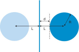
Figure 2: Length scales of the sphere-mirror geometry.

III.1 Large distance expansion

We start by studying the Casimir interaction at large separations. For separations $L$ that are large compared to the size $R$ of the object, the Casimir energy can be expressed as an asymptotic series in $R/L$. Using that $\ln\det=\,{\rm tr}\,\ln$ in Eqs. (II.50) and (II.101), we get by expanding the logarithm

$${\cal E} = \frac{\hbar c}{2\pi}\int_{0}^{\infty}d\kappa\,{\rm tr}\,\ln(1-{\mathbb{N}})$$ (III.1)

$$= -\frac{\hbar c}{2\pi}\int_{0}^{\infty}d\kappa\sum_{p=1}^{\infty}\frac{1}{p}\,{\rm tr}\,\left(\mathbb{N}^{p}\right)\,,$$ (III.2)

where we have defined the operator $\mathbb{N}=\mp\mathbb{T}^{1}\mathbb{U}^{R,11}$ with $-$($+$) for a scalar field in the presence of a Dirichlet (Neumann) mirror and $\mathbb{N}=-\tilde{\mathbb{T}}^{1}\tilde{\mathbb{U}}^{R,11}$ for the electromagnetic field and a perfectly reflecting mirror. The operator ${\mathbb{N}}$ describes a wave that travels from the mirror to the object and back, involving one scattering at the object.

III.1.1 Scalar field

All information about the shape of the surface and the boundary conditions is provided by the ${\mathbb{T}}$-matrix. For a spherically symmetric surface the matrix is diagonal and completely specified by scattering phase shifts $\delta_{l}(k)$ that do not depend on $m$,

$${\mathcal{T}}_{lml^{\prime}m^{\prime}}(k)=\delta_{ll^{\prime}}\delta_{mm^{\prime}}\frac{1}{2}\left(e^{2i\delta_{l}(k)}-1\right)\,,$$ (III.3)

where $k$ is the real frequency. The scattering phase shifts for a sphere of radius $R$ with Dirichlet and Neumann boundary conditions are

$$\cot\delta^{D}_{l}(k) = \frac{n_{l}(\xi)}{j_{l}(\xi)}\,,$$ (III.4)

$$\cot\delta^{N}_{l}(k) = \frac{n^{\prime}_{l}(\xi)}{j^{\prime}_{l}(\xi)}\,,$$ (III.5)

where $\xi=kR$ and $j_{l}$ ($n_{l}$) are spherical Bessel functions of first (second) kind. To make use of the general result of Eq. (II.50), we have to evaluate the matrix elements for imaginary frequencies $k=i\kappa$. This can be done using $j_{l}(iz)=i^{l}\sqrt{\pi/(2z)}I_{l+1/2}(z)$, $h_{l}^{(1)}(iz)=j_{l}(iz)+in_{l}(iz)=-i^{-l}\sqrt{2/(\pi z)}K_{l+1/2}(z)$, where $I_{l+1/2}$ and $K_{l+1/2}$ are modified Bessel functions of first and second kind, respectively. We obtain

$${\mathcal{T}}^{D}_{lmlm} = (-1)^{l}\frac{\pi}{2}\frac{I_{l+1/2}(z)}{K_{l+1/2}(z)}$$ (III.6)

$${\mathcal{T}}^{N}_{lmlm} = (-1)^{l}\frac{\pi}{2}\frac{I_{l+1/2}(z)-2zI^{\prime}_{l+1/2}(z)}{K_{l+1/2}(z)-2zK^{\prime}_{l+1/2}(z)}$$ (III.7)

for Dirichlet and Neumann boundary conditions where $z=\kappa R$.

The distance dependence of the Casimir energy of Eq. (II.50) is given by the translation matrix that describes the interaction between the original and mirror multipole moments. Since the origins (centers) of the original and mirror sphere are related by a translation along the $z$-axis, the matrix elements of the translation matrix ${\mathbb{U}}^{R,11}$ are given by Eqs. (II.28) and (II.29). After a rotation of frequency to the imaginary axis we obtain

$$\mathcal{U}^{R,11}_{l^{\prime}mlm}=-(-1)^{l}i^{-l^{\prime}+l}\sqrt{(2l+1)(2l^{\prime}+1)}\,\sum_{l^{\prime\prime}}\,(-1)^{l^{\prime\prime}}(2l^{\prime\prime}+1)\begin{pmatrix}l&l^{\prime}&l^{\prime\prime}\\ 0&0&0\end{pmatrix}\begin{pmatrix}l&l^{\prime}&l^{\prime\prime}\\ m&-m&0\end{pmatrix}\frac{K_{l^{\prime\prime}+1/2}(2\kappa L)}{\sqrt{\pi\kappa L}}\,.$$ (III.8)

With the elements of the transition and translation matrices we can compute the Casimir interaction from Eq. (II.50). The scaling of the ${\mathbb{T}}$-matrix for small $\kappa$ shows that partial waves of order $l$ start to contribute to the energy at order $L^{-2(l+1)}$ if the ${\mathbb{T}}$-matrix is diagonal in $l$. Hence, we can truncate the infinite matrix ${\mathbb{N}}$ in Eq. (III.1) at finite multipole order to obtain the large distance expansion of the energy at a given order in $R/L$. Also, we can truncate the series over $p$ in Eq. (III.1) since the $p^{\text{th}}$ power of ${\mathbb{N}}$ becomes important only at order $L^{-(p+1)}$. The first $p$ powers of ${\mathbb{N}}$ describe $p$ scattering off the sphere.

We have used Mathematica to perform the matrix operations and to expand the integrand of Eq. (III.1) in $R/L$. From this we find that the Casimir energy can be written as

$${\cal E}=\frac{\hbar c}{\pi}\frac{1}{L}\sum_{j=2}^{\infty}b_{j}\left(\frac{R}{L}\right)^{j-1}\,,$$ (III.9)

where $b_{j}$ is the coefficient of the term $\sim L^{-j}$. In the following we give the results for a mirror plane with Dirichlet or Neumann boundary conditions separately.

Dirichlet mirror — In this case we have $\mathbb{N}=-\mathbb{T}^{1}\mathbb{U}^{R,11}$. If the field obeys Dirichlet boundary conditions at the sphere, we obtain the for leading coefficients

$$b_{2} = -\frac{1}{8},\quad b_{3}=-\frac{5}{64},\quad b_{4}=-\frac{421}{1152},$$

$$\quad b_{5} = -\frac{535}{9216},\quad b_{6}=-\frac{3083041}{4147200},\quad b_{7}=+\frac{2741117}{11059200},$$

$$\quad b_{8} = -\frac{557222415727}{292626432000}\,,$$ (III.10)

indicating an attractive force. This result agrees with recent findings of Wirzba Wirzba:qfext07 . If we impose Neumann boundary conditions at the sphere, we find

$$b_{2} = 0,\quad b_{3}=0,\quad b_{4}=\frac{17}{96},$$

$$\quad b_{5} = 0,\quad b_{6}=\frac{379}{960},\quad b_{7}=\frac{479}{24576},$$

$$\quad b_{8} = \frac{243487}{403200}\,.$$ (III.11)

This result corresponds to a repulsive force which is expected for unlike boundary conditions. To leading order the energy scales as $R^{3}/L^{4}$ since the first two coefficients vanish. This behavior can be understood from the absence of low-frequency $s$-wave scattering for a sphere with Neumann boundary conditions.

Neumann mirror — In this case we have $\mathbb{N}=+\mathbb{T}^{1}\mathbb{U}^{R,11}$. For a Dirichlet sphere we obtain the coefficients

$$b_{2} = \frac{1}{8},\quad b_{3}=\frac{3}{64},\quad b_{4}=\frac{403}{1152},$$

$$\quad b_{5} = \frac{73}{9216},\quad b_{6}=\frac{2981791}{4147200},\quad b_{7}=-\frac{3636227}{11059200},$$

$$\quad b_{8} = \frac{550781720977}{292626432000}\,,$$ (III.12)

and hence the force is again repulsive. The modulus of the coefficients are smaller than those in Eq. (III.1.1) for a Dirichlet mirror with the exception of the leading one, $b_{2}$ and the one with inverted sign, $b_{7}$. Notice that the sum of the Casimir energies for the Dirichlet and Neumann mirror, both opposite to a Dirichlet sphere, is identical to the Casimir energy between two Dirichlet spheres at a center-to-center distance $2L$ Bulgac+06 . The reason for this is that any field configuration can be decomposed into symmetric and antisymmetric modes with respect to the mirror plane which obey Neumann and Dirichlet boundary conditions on that plane, respectively. Since the energy between two spheres scales as $R^{2}/L^{3}$ for asymptotically large separations, the modulus of the coefficients $b_{2}$ in Eqs. (III.1.1) and (III.1.1) must be identical so that the contribution $\sim R/L^{2}$ cancels. It is easily seen that the higher order coefficients of Eqs. (III.1.1) and (III.1.1) combine to the correct coefficients of the large distance expansion for two Dirichlet spheres Emig+07 .

For a Neumann sphere we get

$$b_{2} = 0,\quad b_{3}=0,\quad b_{4}=-\frac{17}{96},$$

$$\quad b_{5} = 0,\quad b_{6}=-\frac{379}{960},\quad b_{7}=-\frac{267}{8192},$$

$$\quad b_{8} = -\frac{243487}{403200}\,.$$ (III.13)

For the same reason as before, the first two coefficients vanish. Notice that all given coefficients, with the exception of $b_{7}$, are equal to minus the corresponding coefficients for a Neumann sphere and a Dirichlet mirror in Eq. (III.1.1). This result is consistent with the observation that the Casimir energy for two Neumann spheres at a center-to-center distance $2L$ is given by the sum of the energies of a Neumann sphere at distance $L$ from a Dirichlet mirror and a Neumann mirror, respectively. Since two Neumann spheres interact at large distance with an energy $\sim R^{6}/L^{7}$ with the next-to-leading term $\sim R^{8}/L^{9}$, the sum of the corresponding coefficients, excepting $b_{7}$, must vanish. The coefficients $b_{7}$ in Eqs. (III.1.1), (III.1.1) combine to the correct value for two Neumann spheres that was obtained in Ref. Emig+07 .

III.1.2 Electromagnetic field

We consider a dielectric sphere at a center-to-surface distance $L$ from a perfectly conducting mirror. Due to spherical symmetry, the electric and magnetic multipoles for all $l$, $m$ are decoupled so that the T-matrix is diagonal Emig+07b ,

$$T^{\textsc{mm}}_{lmlm}=(-1)^{l}\frac{\pi}{2}\frac{\eta I_{l+{1\over 2}}(z)\left[I_{l+{1\over 2}}(nz)+2nzI^{\prime}_{l+{1\over 2}}(nz)\right]-nI_{l+{1\over 2}}(nz)\left[I_{l+{1\over 2}}(z)+2zI^{\prime}_{l+{1\over 2}}(z)\right]}{\eta K_{l+{1\over 2}}(z)\left[I_{l+{1\over 2}}(nz)+2nzI^{\prime}_{l+{1\over 2}}(nz)\right]-nI_{l+{1\over 2}}(nz)\left[K_{l+{1\over 2}}(z)+2zK^{\prime}_{l+{1\over 2}}(z)\right]}\,,$$ (III.14)

where the sphere radius is $R$, $z=\kappa R$, $n=\sqrt{\epsilon(i\kappa)\mu(i\kappa)}$, $\eta=\sqrt{\epsilon(i\kappa)/\mu(i\kappa)}$. $T^{\textsc{ee}}_{lmlm}$ is obtained from Eq. (III.14) by interchanging $\epsilon$ and $\mu$. The limit of a perfectly conducting sphere is obtained by taking $\epsilon(i\kappa)\to\infty$ at an arbitrarily fixed $\mu(i\kappa)$ which can also vanish. Then the matrix elements become independent of $\mu$,

$$T^{\textsc{mm}}_{lmlm} = (-1)^{l}\frac{\pi}{2}\frac{I_{l+{1\over 2}}(z)}{K_{l+{1\over 2}}(z)}$$ (III.15)

$$T^{\textsc{ee}}_{lmlm} = (-1)^{l}\frac{\pi}{2}\frac{I_{l+{1\over 2}}(z)+2zI^{\prime}_{l+{1\over 2}}(z)}{K_{l+{1\over 2}}(z)+2zK^{\prime}_{l+{1\over 2}}(z)}\,.$$ (III.16)

For all partial waves, the leading low frequency contribution is determined by the static electric multipole polarizability, $\alpha^{\textsc{e}}_{l}=[(\epsilon-1)/(\epsilon+(l+1)/l)]R^{2l+1}$, and the corresponding magnetic polarizability, $\alpha^{\textsc{m}}_{l}=[(\mu-1)/(\mu+(l+1)/l)]R^{2l+1}$. Including the next to leading terms, the T-matrix has the structure

$$T^{\textsc{mm}}_{lmlm}=\kappa^{2l}\bigg{[}\frac{(-1)^{l-1}(l+1)\alpha_{l}^{\textsc{m}}}{l(2l+1)!!(2l-1)!!}\kappa+\gamma^{\textsc{m}}_{l3}\kappa^{3}+\gamma^{\textsc{m}}_{l4}\kappa^{4}+\ldots\bigg{]}\,,$$

and $T^{\textsc{ee}}_{lmlm}$ is obtained by $\alpha^{\textsc{m}}_{l}\to\alpha^{\textsc{e}}_{l}$, $\gamma_{ln}^{\textsc{m}}\to\gamma^{\textsc{e}}_{ln}$. The first terms are $\gamma^{\textsc{m}}_{13}=-[4+\mu(\epsilon\mu+\mu-6)]/[5(\mu+2)^{2}]R^{5}$, $\gamma^{\textsc{m}}_{14}=(4/9)[(\mu-1)/(\mu+2)]^{2}R^{6}$, and $\gamma^{\textsc{e}}_{13}$, $\gamma^{\textsc{e}}_{14}$ are obtained again by interchanging $\mu$ and $\epsilon$. Higher order terms can be easily obtained by expanding Eq. (III.14) for small $\kappa$.

The translation matrix elements $\tilde{\mathcal{U}}^{R,11}_{l^{\prime}mlm}=(-1)^{l^{\prime}}\mathcal{U}^{R,11}_{l^{\prime}mlm}$ are obtained from Eqs. (II.81), (II.84) and (II.85). Using $h_{l}^{(1)}(iz)=-i^{-l}\sqrt{2/(\pi z)}K_{l+1/2}(z)$ we get

$$B_{l^{\prime}m^{\prime}lm}(-2L\hat{\bf z}) = -\delta_{m^{\prime}m}(-1)^{m}i^{l-l^{\prime}}\sum_{l^{\prime\prime}}\frac{(-1)^{l^{\prime\prime}}}{2}\left[l(l+1)+l^{\prime}(l^{\prime}+1)-l^{\prime\prime}(l^{\prime\prime}+1)\right]\sqrt{\frac{(2l+1)(2l^{\prime}+1)}{l(l+1)l^{\prime}(l^{\prime}+1)}}(2l^{\prime\prime}+1)$$ (III.17)

$$\times\begin{pmatrix}l&l^{\prime}&l^{\prime\prime}\\ 0&0&0\end{pmatrix}\begin{pmatrix}l&l^{\prime}&l^{\prime\prime}\\ m&-m&0\end{pmatrix}\frac{K_{l^{\prime\prime}+1/2}(2\kappa L)}{\sqrt{\pi\kappa L}}\,,$$

$$C_{l^{\prime}m^{\prime}lm}(-2L\hat{\bf z}) = \delta_{m^{\prime}m}2\kappa Lm(-1)^{m}i^{l-l^{\prime}}\sum_{l^{\prime\prime}}(-1)^{l^{\prime\prime}}\sqrt{\frac{(2l+1)(2l^{\prime}+1)}{l(l+1)l^{\prime}(l^{\prime}+1)}}(2l^{\prime\prime}+1)$$ (III.18)

$$\times\begin{pmatrix}l&l^{\prime}&l^{\prime\prime}\\ 0&0&0\end{pmatrix}\begin{pmatrix}l&l^{\prime}&l^{\prime\prime}\\ m&-m&0\end{pmatrix}\frac{K_{l^{\prime\prime}+1/2}(2\kappa L)}{\sqrt{\pi\kappa L}}\,.$$

Now we can employ the series representation of the Casimir energy in Eq. (III.1) with ${\mathbb{N}}=-\tilde{\mathbb{T}}^{1}\tilde{\mathbb{U}}^{R,11}$. Since the T-matrix is diagonal in $l$, partial waves of order $l$ start to contribute to the energy at order $L^{-2(l+1)}$. Also, the $p^{\text{th}}$ power of ${\mathbb{N}}$ becomes important only at order $L^{-(3p+1)}$. Notice the stronger increase of the exponent with $p$ compared to the scalar case where the exponent is $-(p+1)$. This can be understood from the absence of $s$-waves for the electromagnetic field so that each reflection contributes a factor $1/L^{3}$ due to $p$-waves. Matrix operations and the expansion in $R/L$ are performed with Mathematica. From this we obtain for a dielectric sphere in front of perfectly conducting mirror plane the Casimir energy

$${\cal E} = -\frac{\hbar c}{\pi}\left\{\frac{3}{8}(\alpha_{1}^{\textsc{e}}-\alpha_{1}^{\textsc{m}})\frac{1}{L^{4}}+\frac{15}{32}(\alpha_{2}^{\textsc{e}}-\alpha_{2}^{\textsc{m}}+2\gamma_{13}^{\textsc{e}}-2\gamma_{13}^{\textsc{m}})\frac{1}{L^{6}}+\frac{1}{1024}\left[23(\alpha_{1}^{\textsc{m}})^{2}-14\alpha_{1}^{\textsc{m}}\alpha_{1}^{\textsc{e}}+23(\alpha_{1}^{\textsc{e}})^{2}\right.\right.$$ (III.19)

$$+ \left.\left.2160(\gamma_{14}^{\textsc{e}}-\gamma_{14}^{\textsc{m}})\right]\frac{1}{L^{7}}+\frac{7}{7200}\left[572(\alpha_{3}^{\textsc{e}}-\alpha_{3}^{\textsc{m}})+675\left(9(\gamma_{15}^{\textsc{e}}-\gamma_{15}^{\textsc{m}})-55(\gamma_{23}^{\textsc{e}}-\gamma_{23}^{\textsc{m}})\right)\right]\frac{1}{L^{8}}+\dots\right\}\,.$$

The electric contribution to the leading term, $\sim L^{-4}$, was obtained by Casimir and Polder for the interaction of an atom with static polarizability $\alpha_{1}^{\textsc{e}}$ and a metallic surface Casimir+48 . Later Boyer has generalized the leading order result to include magnetic effects described by $\alpha_{1}^{\textsc{m}}$ Boyer69 . The higher order terms are new. They show how higher order polarizabilities and frequency corrections to the static parameters influence the interaction. There is no $\sim 1/L^{5}$ term. Notice also that the first three terms of the contribution at order $L^{-7}$ have precisely the structure of the Casimir-Polder interaction between two atoms with static dipole polarizabilities $\alpha_{1}^{\textsc{m}}$ and $\alpha_{1}^{\textsc{e}}$ but it is reduced by a factor of $1/2^{8}$. This factor and the distance dependence $\sim L^{-7}$ of this term suggests that it arises from the interaction of the dipole fluctuations inside the sphere with those inside its image at a distance $2L$. The additional coefficient of $1/2$ in the reduction factor $(1/2)(1/2^{7})$ can be traced back to the fact that the forces involved in bringing the dipole in from infinity act only on the dipole and not on its image Barnett+00 .

For a perfectly conducting sphere the coefficients of the expansion of the Casimir energy in $R/L$ become universal numbers. These coefficients can be either obtained from Eq. (III.19) by using the appropriate values of the parameters for a prefect metal or it can be computed directly from the T-matrix elements given in Eqs. (III.15), (III.16). Following the latter route, we get the series

$${\cal E}=\frac{\hbar c}{\pi}\frac{1}{L}\sum_{j=4}^{\infty}b_{j}\left(\frac{R}{L}\right)^{j-1}\,,$$ (III.20)

where the coefficients up to order $1/L^{11}$ are

$$b_{4} = -\frac{9}{16},\quad b_{5}=0,\quad b_{6}=-\frac{25}{32},\quad b_{7}=-\frac{3023}{4096}$$

$$\quad b_{8} = -\frac{12551}{9600},\quad b_{9}=\frac{1282293}{163840},$$

$$b_{10} = -\frac{32027856257}{722534400},\,\,\,b_{11}=\frac{39492614653}{412876800}\,.$$ (III.21)

This and the corresponding results for a scalar field appear to be asymptotic series. Therefore, the series cannot be summed to obtain the interaction at small separations. In the next Section we use a numerical implementation of Eq. (II.101) to compute the interaction at all separations.

III.2 Non-perturbative result at all separations

To obtain the Casimir interaction over a broad range of distances, Eq. (II.101) has to be evaluated numerically. As we employ a partial wave expansion, the computational work increases with decreasing separation between the objects. However, we shall see below that even at small separations our method yields sufficient precision to obtain the leading corrections to the proximity force approximation (PFA). The numerical approach is based on the technique presented in Refs. Emig+07b ; Emig+07 . Using the analytic expressions for the matrix elements of the translation and transition matrices, we compute the determinant and the integral over frequency $\kappa$ in Eq. (II.101) numerically. The matrices are truncated at a finite multipole order $l$ which yields a series of estimates ${\cal E}^{(l)}$ for the Casimir energy. The exact Casimir energy is then obtained by extrapolating the series to $l\to\infty$. For the geometry considered here, we observe an exponentially fast convergence that allows us to obtain accurate results even at small separations from a moderate multipole order.

We compare our results for the interaction energy to the estimate that follows from PFA. This is important since PFA is often used over a range of separations although its accuracy is unknown even at small distances for most geometries, including the electromagnetic Casimir interaction between a plane and a sphere. The PFA estimate for the latter geometry is given by

$${\cal E}_{\text{PFA}}=\pi\Phi_{0}^{\pm/\text{EM}}\,\frac{\hbar c\,R}{d^{2}}$$ (III.22)

where $d=L-R$ is the surface-to-surface distance. The amplitudes follow from the result for two parallel plates and are given by

$$\Phi_{0}^{-} = -\frac{\pi^{2}}{1440}$$ (III.23)

$$\Phi_{0}^{+} = +\frac{7\pi^{2}}{11520}$$ (III.24)

$$\Phi_{0}^{\text{EM}} = -\frac{\pi^{2}}{720}$$ (III.25)

for a scalar field with like ($-$) and unlike ($+$) boundary conditions and the electromagnetic field, respectively. In the following we present our results for the plane-sphere interaction over a wide range of separations for scalar fields with Dirichlet and Neumann boundary conditions and for the electromagnetic field.

III.2.1 Scalar field

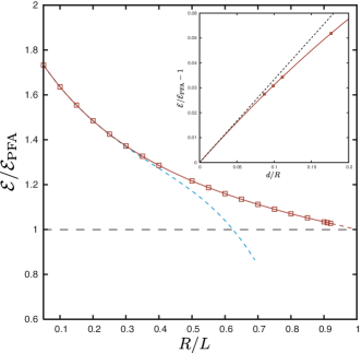
Figure 3: Sphere-plane Casimir interaction of a scalar field with Dirichlet boundary conditions on both surfaces. The energy is scaled by the PFA estimate of Eq. (III.22). The dashed curve represents the large distance expansion of Eq. (III.9) with the coefficients of Eq. (III.1.1). Inset: Corrections to the PFA at small separations as function of the surface-to-surface distance $d=L-R$. The dashed curve corresponds to the lowest order correction to the PFA obtained by Bordag Bordag:qfext07 .

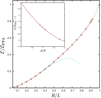
Figure 4: Analog of Fig. 3 for Neumann boundary conditions at the sphere and the plane. The dashed curve represents the large distance expansion of Eq. (III.9) with the coefficients of Eq. (III.1.1).

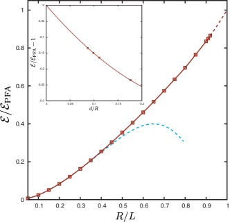
Figure 5: Analog of Fig. 3 for Neumann boundary conditions at the sphere and Dirichlet boundary conditions at the plane. The dashed curve represents the large distance expansion of Eq. (III.9) with the coefficients of Eq. (III.1.1).

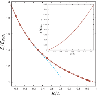
Figure 6: Analog of Fig. 3 for Dirichlet boundary conditions at the sphere and Neumann boundary conditions at the plane. The dashed curve represents the large distance expansion of Eq. (III.9) with the coefficients of Eq. (III.1.1).

We consider the four cases that correspond to Dirichlet or Neumann boundary conditions at the sphere and the mirror plane. The results for the Casimir energy are shown in Figs. 3-6. At large separations the results of the numerical evaluation of the determinant agree nicely with the large distance expansions of the previous section. For a sphere with Dirichlet boundary conditions, the energy scales both at large and small separations as $R/d^{2}$ so that the curves for ${\cal E}/{\cal E}_{\text{PFA}}$ in Figs. 3 and 6 tend also to a constant for $R/L\to 0$. The PFA underestimates the actual interaction energy at all separations. For a Neumann sphere the interaction scales at large separations as $R^{3}/L^{4}$ so that the curves for ${\cal E}/{\cal E}_{\text{PFA}}$ in Figs. 4 and 5 tend to zero for $R/L\to 0$. Here the PFA overestimates the actual interaction energy at all separations.

The non-perturbative approach allows us to study also the case of small separations. In that limit our results can be fitted to a power law of the form

$${\cal E}={\cal E}_{\text{PFA}}\left[1+\theta_{1}\frac{d}{R}+\theta_{2}\left(\frac{d}{R}\right)^{2}+\ldots\right]\,.$$ (III.26)

The coefficients $\theta_{j}$ obtained from a fit of the function of Eq. (III.26) to the data points for the four smallest studied separations are summarized in Tab. 1. The fitted curves are shown as insets in Figs. 3-6. The result for $\theta_{1}$ for the case of Dirichlet boundary conditions at the sphere and the mirror agrees with the analytical result $\theta_{1}=1/3$ presented in Ref. Bordag:qfext07 . Again for Dirichlet conditions, for the second order coefficient a considerably larger numerical estimate of $\theta_{2}=1.92$ has been obtained from world-line Monte Carlo sampling Gies+06a ; Gies+06b . For the other combinations of boundary conditions our findings represent the first results for the corrections to the PFA.

boundary condition	$\theta_{1}$	$\theta_{2}$
plane / sphere
D / D	$0.3346\pm 0.0017$	$-0.231\pm 0.012$
N / N	$-2.4298\pm 0.0070$	$4.394\pm 0.049$
D / N	$-1.7493\pm 0.0061$	$2.354\pm 0.042$
N / D	$0.1124\pm 0.0043$	$1.240\pm 0.044$
EM / EM	$-1.42\pm 0.02$	$2.39\pm 0.14$

Table 1: Coefficients describing corrections to PFA, see Eq. (III.26). D=Dirichlet, N=Neumann (scalar field) and EM=perfectly conducting boundary conditions (electromagnetic field).

III.2.2 Electromagnetic field

We focus on a perfectly conducting sphere and mirror plane. The Casimir energy resulting from a numerical computation of the determinant of Eq. (II.101) is shown for a wide range of separations in Fig. 7. At large separations the interaction is described by the asymptotic result of Eq. (III.20). At small distances the Casimir energy approaches to PFA estimate and corrections to PFA can be described again by Eq. (III.26). A corresponding fit to the data points for the four smallest separations is shown as inset in Fig. 7. The corresponding amplitudes of the correction terms are listed in Tab. 1.

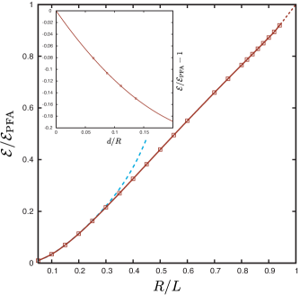
Figure 7: Electromagnetic Casimir energy for the sphere-plate geometry. The energy is scaled by the PFA estimate of Eq. (III.22). The asymptotic expansion of Eq. (III.20) to order $1/L^{10}$ is shown as dashed line. Inset: Corrections to the PFA at small distances as function of $d=L-R$.

This result is important for a number of recent measurements of the Casimir force between almost flat surfaces. These experiments have been performed for a plane mirror and a sphere with a radius that is much larger than the distance between the surfaces in order to avoid difficulties from parallelism control. Our results at short distances indicate that for a sphere of radius $R=100\mu$m the corrections to PFA are below $1\%$ only for surface-to-surface distances $d$ that are smaller than $\approx 700$nm. For a sphere of that size, PFA fails already by $10\%$ at a distance of $\approx 8\mu$m. From this we conclude that the currently achieved experimental accuracy for measurements of Casimir forces in the sphere-plate geometry with a sphere of $R=100\mu$m at distances below $d=1\mu$m is within the range or slightly less than the corrections to PFA.

However, deviations from PFA become severe when smaller objects interact with surfaces. Hence it is important to understand the crossover of the Casimir interaction between macroscopic objects and the eventual Casimir-Polder interaction between single atoms and a surface. A description of this crossover is provided by our results in Fig. 7. Corresponding results can be also obtained for a dielectric sphere or less symmetric objects by the methods presented here. Finally, we note that it should be also possible to compute correction amplitudes like the $\theta_{j}$ in Eq. (III.26) analytically by applying methods similar to those used in Ref. Bordag06 . However, the validity range of the corresponding series would be limited to small separations and for an overall description of the interaction one should resort to the device of a numerical evaluation along the lines presented here.

IV Acknowledgments

This work emerged from a collaboration with R. L. Jaffe, M. Kardar, and N. Graham on related problems. Support by the Heisenberg program of the Deutsche Forschungsgemeinschaft is acknowledged.

References

- (1) T. Emig, N. Graham, R. L. Jaffe, and M. Kardar, Phys. Rev. Lett. 99, 170403 (2007).
- (2) T. Emig, N. Graham, R. L. Jaffe, and M. Kardar, Preprint arXiv:0710:3084.
- (3) H. B. G. Casimir, Indag. Math. 10, 261 (1948) [Kon. Ned. Akad. Wetensch. Proc. 51, 793 (1948)].
- (4) S. K. Lamoreaux, Phys. Rev. Lett. 78, 5 (1997).
- (5) U. Mohideen and A. Roy, Phys. Rev. Lett. 81, 4549 (1998).
- (6) A. Roy et al., Phys. Rev. D 60, 111101(R) (1999).
- (7) T. Ederth, Phys. Rev. A 62, 062104 (2000).
- (8) H. B. Chan et al., Science 291, 1941 (2001).
- (9) F. Chen et al., Phys. Rev. Lett. 88, 101801 (2002).
- (10) F. Chen, G. L. Klimchitskaya, V. M. Mostepanenko, and U. Mohideen, Phys. Rev. Lett. 97, 170402 (2006).
- (11) R. S. Decca, D. López, E. Fischbach, G. L. Klimchitskaya, D. E. Krause, and V. M. Mostepanenko, Phys. Rev. D 75, 077101 (2007).
- (12) F. Chen, G. L. Klimchitskaya, V. M. Mostepanenko, and U. Mohideen, Phys. Rev. B 76, 035338 (2007).
- (13) J. N. Munday and F. Capasso, Phys. Rev. A 75, 060102(R) (2007).
- (14) V. A. Parsegian, Van der Waals forces, Cambridge Univ. Press (2005).
- (15) H. B. G. Casimir and D. Polder, Phys. Rev. 73, 360 (1948).
- (16) D. M. Harber, J. M. Obrecht, J. M. McGuirk, and E. A. Cornell, Phys. Rev. A 72, 033610 (2005).
- (17) D. E. Krause, R. S. Decca, D. López, and E. Fischbach, Phys. Rev. Lett. 98, 050403 (2007).
- (18) A. Rodriguez, M. Ibanescu, D. Iannuzzi, F. Capasso , J. D. Joannopoulos and S. G. Johnson, Phys. Rev. Lett. 99, 080401 (2007); A. Rodriguez, M. Ibanescu, D. Iannuzzi, J. D. Joannopoulos, and S. G. Johnson, Phys. Rev. A 76, 032106 (2007).
- (19) S. J. Rahi, A. W. Rodriguez, T. Emig, R. L. Jaffe, S. G. Johnson, M. Kardar, arXiv:0711.1987 (2007).
- (20) R. Balian and B. Duplantier, Ann. Phys. (New York) 104, 300 (1977); 112, 165 (1978).
- (21) M. T. Jaeckel, S. Reynaud, J. de Physique I 1 1395 (1991).
- (22) T. Emig, R. Büscher, Nucl. Phys. B696, 468 (2004).
- (23) A. Lambrecht, P.A. Maia Neto and S. Reynaud, New J. Phys. 8, 243 (2006).
- (24) P. A. Maia Neto, A. Lambrecht and S. Reynaud, Europhys. Lett. 69, 924 (2005); Phys. Rev. A 72, 012115 (2005).
- (25) T. Emig, R. L. Jaffe, M. Kardar, A. Scardicchio, Phys. Rev. Lett. 96, 080403 (2006).
- (26) M. Bordag, Phys.Rev. D 73, 125018 (2006).
- (27) O. Kenneth and I. Klich, Phys. Rev. Lett. 97, 160401 (2006).
- (28) O. Kenneth and I. Klich, arXiv:0707.4017 (2007).
- (29) A. Bulgac, P. Magierski, and A. Wirzba, Phys. Rev. D 73, 025007 (2006).
- (30) A. Wirzba, arXiv:0711.2395 (2007).
- (31) H. Gies and K. Klingmüller, Phys. Rev. Lett. 97, 220401 (2006).
- (32) H. Gies and K. Klingmüller, Phys. Rev. D 74, 045002 (2006).
- (33) M. Bordag, D. Robaschik, and E. Wieczorek, Ann. Phys. 165, 192 (1985).
- (34) H. Li and M. Kardar, Phys. Rev. Lett. 67, 3275 (1991); Phys. Rev. A 46, 6490 (1992).
- (35) R. C. Wittmann, IEEE Trans. Antennas Propagat. 36, 1078 (1988).
- (36) T. H. Boyer, Phys. Rev. 180, 19 (1969).
- (37) S. Barnett, A. Aspect, and P. W. Milonni, J. Phys. B: At. Mol. Opt. Phys. 33, L143 (2000).
- (38) M. Bordag, Talk presented at the workshop QFEXT07, Leipzig, September 2007.