Vehicular traffic flow at a non-signalised intersection

Abstract

We have developed a modified Nagel-Schreckenberg cellular automata model for describing a conflicting vehicular traffic flow at the intersection of two streets. No traffic lights control the traffic flow. The approaching cars to the intersection yield to each other to avoid collision. Closed boundary condition is applied to the streets. Extensive Monte Carlo simulations is taken into account to find the model characteristics. In particular, we obtain the fundamental diagrams and show that the effect of interaction of two streets can be regarded as a dynamic impurity located at the intersection point. Our results suggest that yielding mechanism gives rise to a high total flow throughout the intersection especially in the low density regime. In some ranges of densities, yielding mechanism even improves and regulates the flow in comparison to the absence of perpendicular flow.

Keywords: Traffic flow, Intersection, Signalisation.

I Introduction

Modeling the dynamics of vehicular traffic flow has constituted the subject of intensive research by statistical physics and applied mathematics communities during the past years kernerbook ; schadrev ; helbingrev ; klar ; bellom . In particular, cellular automata approach have provided the possibility to study various aspects of these truly non-equilibrium systems which still are of current interest tgf01 ; tgf03 ; tgf05 . Besides various theoretical efforts aiming to understand the basic principles governing the spatial-temporal structure of traffic flow, considerable attempts have been made towards realistic problems involving optimization of vehicular traffic flow. While the existing results in the context of highway traffic seem to need further manipulations in order to find direct applications, researches on city traffic have more feasibility in practical applications bml ; nagatani ; tadaki1 ; tadaki2 ; cuesta ; torok ; freund ; cs ; brockfeld . We believe that optimisation of traffic flow at a single intersection is a substantial ingredient for the task of global optimisation of city networks chitur . Isolated intersections are fundamental operating units of complex city networks and their thorough analysis would be inevitably advantageous not only for optimisation of city networks but also for local optimization purposes. Recently, physicists have paid notable attention to controlling traffic flow at intersections and other traffic designations such as roundabouts foolad1 ; foolad2 ; foolad3 ; foolad4 ; helbing1 ; helbing2 ; helbing3 ; ray ; xiong ; gershenson . In this respect, our objective in this paper is to study another aspect of conflicting traffic flow at intersections. In principle, the vehicular flow at the intersection of two roads can be controlled via two distinctive schemes. In the first scheme, which is appropriate when the density of cars in both roads are low, the traffic is controlled without traffic lights. In the second scheme, signalized traffic lights control the flow. In the former scheme, approaching car to the intersection yield to traffic at the perpendicular direction by adjusting its velocity to a safe value to avoid collision. According to driving rules, the priority is given to the nearest car to the intersection. It is evident that this scheme is efficient if the density of cars is low. When the density of cars increases, this method fails to optimally control the traffic and long queues may form which gives rise to long delays. At this stage the implementation of the second scheme i.e.; utilizing traffic lights is unavoidable. Therefore it is a natural and important question to find out under what circumstances the intersection should be controlled by traffic lights? More concisely, what is the critical density beyond which the non-signalised schemes begins to fail. In order to capture the basic features of this problem, we have constructed a cellular automata model describing the above dynamics. This paper has the following layout. In section II, the model is introduced and driving rules are explained. In section III, the results of the Monte Carlo simulations are exhibited. Concluding remarks and discussions ends the paper in section IV.

II Description of the Problem

We now present our CA model. Consider two perpendicular one dimensional closed chains each having $L$ sites. The chains represent urban roads accommodating unidirectional vehicular traffic flow. They cross each other at the sites $i_{1}=i_{2}=\frac{L}{2}$ on the first and the second chain respectively. With no loss of generality we take the direction of traffic flow in the first chain from south to north and in the second chain from east to west (see Fig.1 for illustration). The discretisation of space is such that each car occupies an integer number of cells denoted by $L_{car}$. The car position is denoted by the location of its head cell. Time elapses in discrete steps of $\Delta t$ $sec$ and velocities take discrete values $0,1,2,\cdots,v_{max}$ in which $v_{max}$ is the maximum velocity of cars.

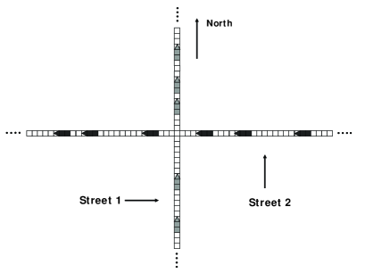
Figure 1: Intersection of two uni-directional streets.

To be more specific, at each step of time, the system is characterized by the position and velocity configurations of cars. The system evolves under the Nagel-Schreckenberg (NS) dynamics ns . Let us briefly explain the NS updating rules which synchronously evolve the system state from time $t$ to $t+1$. We denote position, velocity and space gap of a typical car at timestep t by $x^{(t)},v^{(t)}$ and $g^{(t)}$ respectively. The same quantities for its leading car are correspondingly denoted by $x_{l}^{(t)},v_{l}^{(t)}$ and $g_{l}^{(t)}$. We recall that gap is defined as the distance between front bumper of the follower to the rear bumper of its leading. More precisely, $g(t)=x_{l}(t)-x(t)-L_{car}$. Concerning the above considerations, the following updating sub steps evolve the position

and the velocity of each car in parallel.

1) Acceleration:

$v^{(t+1/3)}:=min(v^{(t)}+1,v_{max})$

2) Velocity adjustment :

$v^{(t+2/3)}:=min(g^{(t+1/3)},v^{(t+1/3)})$

3) Random breaking with probability $p$:

if random $<p$ then $v^{(t+1)}:=max(v^{(t+2/3)}-1,0)$

4) Movement : $x^{(t+1)}:=x^{(t)}+v^{(t+1)}$

The yielding dynamics in the vicinity of the intersection is implemented by introducing a safety distance $D_{s}$. The approaching cars (nearest cars to the crossing point $i=\frac{L}{2}$) should yield to each other if their distances to the crossing point, denoted by $d_{1}$ and $d_{2}$ for the first and second street respectively, are both less than the safety distance $D_{s}$. In this case, the movement priority is given to the car which is closer to the crossing point. This car adjust its velocity as usual with its leading car. On the contrary, the further car, which is the one that should yield, brakes irrespective of its direct gap. The simplest way to take into this cautionary braking is to adjust the gap with the crossing point itself. This implies that the yielding car sees the crossing point as a hindrance. In this way, the model is collision-free. Figure two illustrates the situation.

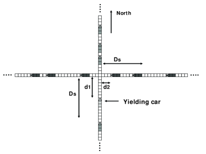
Figure 2: Two approaching cars to the intersection yield to each other provided their distances to the crossing point are both less than a safety distance.

Let us now specify the physical values of our time and space units. Ignoring the possibility of existence of long vehicles such as buses, trucks etc, the length of each cell is taken to be as 4.5 metres which is the typical bumper-to-bumper distance of cars in a waiting queue. Therefore the spatial grid $\Delta x$ equals to $\frac{4.5}{L_{car}}~{}m$. We take the time step $\Delta t=1~{}s$. Furthermore, we adopt a speed-limit of $75~{}km/h$. The value of $v_{max}$ is so chosen to give the speed-limit value $75~{}km/h$ or equivalently $21~{}m/s$ . In this regard, $v_{max}$ is given by the integer party of $21\times L_{car}/4.5$. For instance, for $L_{car}=5$, $v_{max}$ equals $23$. In addition, each discrete increments of velocity signifies a value of $\Delta v=\frac{4.5}{L_{car}}m/s$ which is also equivalent to the acceleration. For $L_{car}=5$ this gives the comfort acceleration $0.9~{}\frac{m}{s^{2}}$. Moreover, we take the value of random breaking parameter at $p=0.1$. In the next section, the simulation results of the above-described dynamics is presented.

III Monte Carlo simulation

The streets sizes are equally taken as $L_{1}=L_{2}=1350~{}m$ and the system is update for $10^{6}$ time steps. After transients, two streets maintain steady-state currents, defined as the number of vehicles passing from a fixed location per a definite time interval, denoted by $J_{1}$ and $J_{2}$ . They are functions of the global densities $\rho_{1}=\frac{N_{1}\times L_{car}}{L_{1}}$ and $\rho_{2}=\frac{N_{2}\times L_{car}}{L_{2}}$ where $N_{1}$ and $N_{2}$ are the number of vehicles in the first and the second street respectively. We kept the global density at a fixed value $\rho_{2}$ in the second street and varied $\rho_{1}$. Figure (3) exhibits the fundamental diagram of the first street i.e.; $J_{1}$ versus $\rho_{1}$.

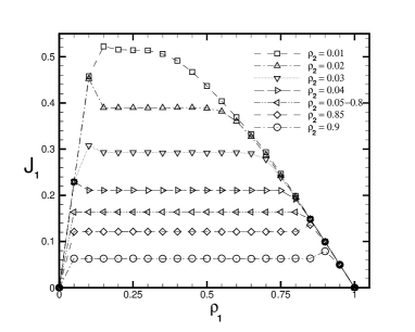
Figure 3: $J_{1}$ vs $\rho_{1}$ for various values of $\rho_{2}$. $D_{s}=25~{}m$ and $L_{car}=5$ cells. The road length is $1350$ metre.

It is observed that for small densities $\rho_{2}$ up to $0.05$, $J_{1}$ rises to its maximum value, then it undergoes a short rapid decrease after which a lengthy plateau region, where the current is independent of $\rho_{1}$, is formed. Intersection of two chains makes the intersection point appear as a site-wise dynamical defective site. It is a well-known fact that a local defect can affect the low dimensional non-equilibrium systems on a global scale lebowitz ; evans1 ; barma1 ; kolomeisky1 ; krug ; chou ; lakatos1 ; foolad5 ; kerner . This has been confirmed not only for simple exclusion process but also for cellular automata models describing vehicular traffic flow chung ; yukawa . Analogous to static defects, in our case of dynamical impurity, we observe that the effect of the site-wise dynamic defect is to form a plateau region $\rho\in[\rho_{-},\rho_{+}]$ in which $\Delta=\rho_{+}-\rho_{-}$ is the extension of the plateau region in the fundamental diagram. The larger the density in the perpendicular chain is, the more strong is the dynamic defect. For higher $\rho_{2}$, the plateau region is wider and the current value is more reduced. After the plateau, $J_{1}$ exhibits linear decrease versus $\rho_{1}$ in the same manner as in the fundamental diagram of a single road. In this region which corresponds to $\rho_{1}>\rho_{+}$ the intersecting road imposes no particular effect on the first road. Increasing $\rho_{2}$ beyond $0.05$ gives rise to substantial changes in the fundamental diagram. Contrary to the case $\rho_{2}<0.05$, the abrupt drop of current after reaching its maximum disappears for $\rho_{2}>0.05$ and $J_{1}$ reaches its plateau value without showing any decrease. The length and height of the plateau does not show significant dependence for $\rho_{2}\in[0.05,0.8]$. This marks the efficiency of the non signalised controlling mechanism in which the current of each street is highly robust over the density variation in the perpendicular street. When $\rho_{2}$ exceeds $0.8$, the plateau undergoes changes. Its length increases whereas its height decreases. We now consider the flow characteristics in the second street. Although the global density is constant in street $2$ its current $J_{2}$ is affected by density variations in the first street. In Figure (4) we depict the behaviour of $J_{2}$ versus $\rho_{1}$.

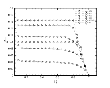
Figure 4: $J_{2}$ vs $\rho_{1}$ for various values of $\rho_{2}$. $D{s}=25~{}m$ and $L_{car}=5$ cells. The road length is $1350$ metre.

For each value of $\rho_{2}$, the current $J_{2}$ as a function of $\rho_{1}$ exhibits three regimes. In the first regime in which $\rho_{1}$ is small, $J_{2}$ is a decreasing function of $\rho_{1}$. Afterwards, $J_{2}$ reaches a plateau region (second regime) which is approximately extended over the region $\rho_{1}\in[0.1,0.8]$. Eventually in the third regime, $J_{2}$ exhibits decreasing behaviour towards zero. Analogous to $J_{1}$, the existence of wide plateau regions indicates that street $2$ can maintain a constant flow capacity for a wide range of density variations in the first street. The other feature is that in fixed $\rho_{1}$, $J_{2}$ is an increasing function for small values of $\rho_{2}$. This is natural since the current in street $2$ has not reached its maximal value. This increment persists up to $\rho_{2}=0.05$. Beyond that, for each $\rho_{1}$, $J_{2}$ saturates. In the plateau region, the saturation value is slightly above $0.16$. The current saturation continues up to $\rho_{2}=0.8$ above which $J_{2}$ again starts to decrease. We note that the behaviours depicted in $J_{1}-\rho_{1}$ and $J_{2}-\rho_{1}$ diagrams are consistent to each other. Due to the existence of $1\rightleftharpoons 2$ symmetry, the $J_{2}-\rho_{2}$ diagram is identical to $J_{1}-\rho_{1}$ and $J_{1}-\rho_{2}$ is identical to $J_{2}-\rho_{1}$. In order to find a deeper insight, it would be illustrative to look at the behaviour of total current $J_{tot}=J_{1}+J_{2}$ as a function of density in one of the streets. Fig. (5) sketches this behaviour.

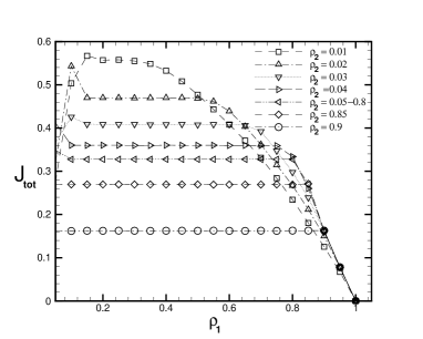
Figure 5: Total current $J_{tot}$ vs $\rho_{1}$ for various values of $\rho_{2}$. $D_{s}=25~{}m$ and $L_{car}=5$ cells.

For $\rho_{2}<0.05$, the maximum of $J_{tot}$ lies at $\rho_{1}=0.1$. However, for $\rho_{2}>0.05$, the maximum shifts backward to $\rho_{1}=0$. According to the above graphs, after a short increasing behaviour, $J_{tot}$ enters into a lengthy plateau region. Evidently for optimisation of traffic one should maximize the total current $J_{tot}$. The existence of a wide plateau region in $J_{tot}$ suggests that yielding mechanism can be regarded as an efficient method in the plateau range of density in the first street. Let us now consider the role of $L_{car}$. The cellular nature of our model permits us to adjust the cell length $\Delta x$ in such a way to reproduce a reasonable acceleration. Our simulations demonstrate that currents exhibit significant dependence on $\Delta x$ or equivalently on $L_{car}$. This is exhibited in figures (6,7).

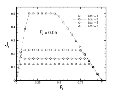
Figure 6: $J_{1}$ vs $\rho_{1}$ for various $L_{car}$. Global density of the second street is kept fixed at $\rho_{2}=0.05$.

While the structure of the fundamental diagram does not qualitatively change, the values of $J_{1}$ notably depend on $L_{car}$. For both $\rho_{2}=0.05$ and $0.5$, $J_{1}$ is a decreasing function of $L_{car}$. The reason is that larger $L_{car}$ gives rise to higher acceleration.

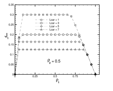
Figure 7: $J_{1}$ vs $\rho_{1}$ for various $L_{car}$ with $\rho_{2}=0.5$.

Analogous to $J_{1}$, the dependence of $J_{2}$ on $L_{car}$ is considerable as is shown in figures (8,9). Variation of $L_{car}$ does not lead to change the generic behaviour but rather changes the current values. Due to the same reason which was explained, smaller $L_{car}$ gives higher currents. In the case $L_{car}=1$, the transition of $J_{2}$ from the plateau region to the linear decreasing segment is much smoother compared to the other values of $L_{car}$ greater than one. Since the currents in the plateau region do not depend on density, therefore the higher acceleration gives rise to larger currents.

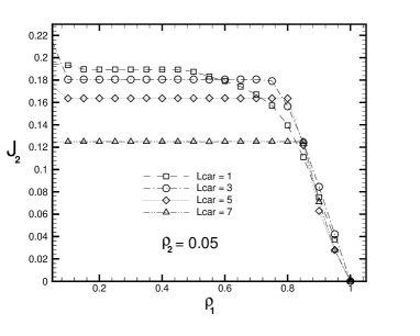
Figure 8: $J_{2}$ versus $\rho_{1}$ for various $L_{car}$. $\rho_{2}=0.05$.

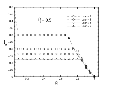
Figure 9: $J_{2}$ versus $\rho_{1}$ for various $L_{car}$. The density is kept fixed in the second street at $\rho_{2}=0.5$ .

Finally, we have also examined the effect of varying the safety distance $D_{s}$. Our simulations do not show any significant dependence on $D_{s}$. This is due to unrealistic decceleration in the NS model.

IV Summary and Concluding Remarks

We have investigated the flow characteristics of a non signalised intersection by developing a Nagel-Schreckenberg cellular automata model. In particular, we have obtained the fundamental diagrams in both streets. Our findings show yielding of cars upon reaching the intersection gives rise to formation of plateau regions in the fundamental diagrams. This is reminiscent of the conventional role of a single impurity in the one dimensional out of equilibrium systems. The performance of non-signalised controlling mechanism is especially efficient when the car density is considerably low in both streets. The existence of wide plateau region in the total system current shows the robustness of the controlling scheme to the density fluctuations and offers an optimal method for controlling the traffic at low densities. Our CA model allows for varying space and time grids. By their appropriate adjusting, we are able to reproduce a realistic acceleration. In low densities, the currents exhibits notable dependence on the values of spatial discretisation grid. Finally we remark that our approach is open to serious challenges. The crucial point is to model the yielding braking as realistic as possible. Empirical data are certainly required for this purpose. We expect the system characteristics undergo substantial changes if realistic yielding declaration is taken into account.

V acknowledgement

We highly appreciate Kadkhodaa Yaghoub, Sardaar Kaamyaab and Mehdi Neek Amal for their useful helps .

References

- (1) B. Kerner, Physics of traffic flow, Springer (2004).
- (2) D. Chowdhury, L. Santen and A. Schadschneider, Physics Reports , 329, 199 (2000).
- (3) D. Helbing, Rev. Mod. Phys., 73, 1067 (2001).
- (4) A. Klar, R.D. Küne and R. Wegener Survey Math. Ind., 6, 215 (1996).
- (5) N. N. Bellomo, M. Delitala and V. Coscia Mathematical Models an Methods in Applied Scinces, 12, 1801 (2002).
- (6) M. Fukui, Y. Sugiyama, M. Schreckenberg and D.E. Wolf (eds.) Traffic and Granular flow 01, (Springer, 2003).
- (7) Serge P. Hoogendoorn, Stefan Luding, Piet H. L. Bovy, M. Schreckenberg and D.E. Wolf (eds.) Traffic and Granular flow 03, (Springer, 2005).
- (8) R. Küne, A. Schadschneider, M. Schreckenberg and D.E. Wolf (eds.) Traffic and Granular flow 05, (Springer, 2007).
- (9) O. Biham, A. Middleton and D. Levine, Phys. Rev. A, 46, R6124 (1992).
- (10) T. Nagatani, J. Phys. Soc. Japan, 63, 1228 (1994); J. Phys. Soc. Japan, 64, 1421 (1995); T. Nagatani and T. Seno, Physica A, 207, 574 (1994).
- (11) S. Tadaki, and M. Kikuchi J. Phys. Soc. Japan, 64, 4504 (1995); Phys. Rev. E, 50, 4564 (1994).
- (12) S. Tadaki, Phys. Rev. E, 54, 2409 (1996); J. Physi. Soc. Jpn. 66, 514 (1997).
- (13) J.A. Cuesta, F.C. Martines, J.M. Molera and A. Sanchez, Phys. Rev. E, 48, R4175 (1993).
- (14) J. Török and J. Kertesz, Physica A, 231, 515 (1996).
- (15) J. Freund and T. Pöschel, Physica A, 219, 95 (1995).
- (16) D. Chowdhury and A. Schadschneider, Phys. Rev. E, 59 , R 1311 (1999).
- (17) E. Brockfeld, R. Barlovic, A. Schadschneider and and M. Schreckenberg, Phys. Rev. E, 64, 056132 (2001).
- (18) Y. Chitur and B. Piccoli, Discrete and Continuous Dynamical Systems B, 5, 599 (2005).
- (19) M.E. Fouladvand and M. Nematollahi, Eur. Phys. J. B, 22, 395 (2001).
- (20) M. E. Fouladvand, Z. Sadjadi and M. R. Shaebani J. Phys. A: Math. Gen, 37, 561 (2004).
- (21) M. E. Fouladvand, Z. Sadjadi and M. R. Shaebani Phys. Rev. E, 70, 046132 (2004).
- (22) M. E. Fouladvand, M. R. Shaebani and Z. Sadjadi J. Phys. Soc. Japan, 73, No. 11, 3209 (2004).
- (23) D. Helbing, S. Lmmer and J.P. Lebacque, in C. Deissenberg and R.F. Hartl(eds.), Optimal Control and Dynamic Games, p. 239, Springer, Dortrecht,2005; arXive physics/0511018.
- (24) S. Lmmer, H. Kori, K. Peters and D. Helbing, Physica A, 363, 39 (2006).
- (25) R. Jiang, D. Helbing, P. Kumar Shukla and Q-S Wu; arXive: condmat/0501595.
- (26) B. Ray and S.N. Bhattacharyya, Phys. Rev. E, 73, 036101 (2006).
- (27) C. Rui-Xiong, Bai Ke- Zhao and L. Mu-Ren, Chinese Physics, 15, No 7, July 2006.
- (28) S-B Cools, C. Gershenson and B. D Hooghe, arXive: nlin.AO/0610040
- (29) K. Nagel, M. Schreckenberg, J.Phys. I France, 2, 2221 (1992).
- (30) S. Janowsky and J. Lebowitz Phys. Rev. A, 45, 618 (1992).
- (31) M. R. Evans, J. Phys. A: Math,Gen., 30, 5669 (1997).
- (32) G. Tripathy and M. Barma, Phys. Rev. Lett., 78, 3039 (1997).
- (33) A. B. Kolomeisky, J. Phys. A: Math, Gen., 31, 1153 (1998).
- (34) M. Bengrine, A. Benyoussef, H. Ez-Zahraouy, J. Krug, M. Loulidi and F. Mhirech J. Phys. A: Math,Gen., 32, 2527 (1999).
- (35) T. Chou and G. Lakatos, Phys. Rev. Lett., 93, 198101 (2004).
- (36) G. Lakatos, T. Chou and A. B. Kolomeisky, Phys. Rev. E, 71, 011103 (2005).
- (37) M. E. Foulaadvand, S. Chaaboki and M. Saalehi, Phys. Rev. E, 75, 011127 (2007).
- (38) B. S. Kerner, Phyisca A, 355, 565 (2005).
- (39) K.H. Chung and P.M. Hui, J. Phys. Soc. Jap., 63, 4338 (1994).
- (40) S. Yukawa, M. Kikuchi and S. Tadaki J. Phys. Soc. Jap., 63, 3609 (1994).