Analysis of vibration impact on stability of dewetting thin liquid film

Abstract

Dynamics of a thin dewetting liquid film on a vertically oscillating substrate is considered. We assume moderate vibration frequency and large (compared to the mean film thickness) vibration amplitude. Using the lubrication approximation and the averaging method, we formulate the coupled sets of equations governing the pulsatile and the averaged fluid flows in the film, and then derive the nonlinear amplitude equation for the averaged film thickness. We show that there exists a window in the frequency-amplitude domain where the parametric and shear-flow instabilities of the pulsatile flow do not emerge. As a consequence, in this window the averaged description is reasonable and the amplitude equation holds.

The linear and nonlinear analyses of the amplitude equation and the numerical computations show that such vibration stabilizes the film against dewetting and rupture.

I Introduction

Studies of stability, dewetting and rupture of thin liquid films on solid substrates are of great importance for micro- and nanotechnologies. Since the first works appeared in 1960s and 1970s, these subjects continue to attract enormous attention, see for instance Refs. TMP ; IM ; GKS ; PRB ; WB ; SHJ1 ; GRP ; GW ; BPT ; LW . Refs. Oron and  SHJ are the reviews of recent results in this extremely diverse field.

The subject of this paper is the general theoretical investigation of the impact of the vibration on the stability of a thin dewetting liquid film. Our interest in studying vibration impacts stems from the large body of works in fluid mechanics of macroscopic fluid layers, including Refs. wolf-69 ; wolf-70 ; Kozlov-98 ; Kozlov-01 (the experiment) and Refs. TVC ; LChbook ; Lapuerta ; Thiele ; Khenner (the theory and numerical modeling), where the vibration is shown to drastically affect the stability characteristics and the dynamics of fluid surfaces and interfaces.

In this paper we assume that the external influences on the film are the vibration, the gravity, and the long-range molecular attraction by the planar substrate, typified by van der Waals forces. Other effects (such as, for instance, the thermocapillarity and the evaporation) can be easily included by simply adding the corresponding terms to the final evolution equation for the film thickness.

The theory we develop is based on the standard longwave lubrication approximation, as discussed by Oron, Davis, and Bankoff Oron , and on the time-averaging method. The general discussion of the averaging methods can be found in Refs. S ; AverBook ; Nayfeh . The key idea is the separation of the dynamics onto fast pulsations and slow relaxation processes. This approach works well when the vibration frequency is high in a certain sense, i.e. when there exists a large difference in the characteristic times (such as the viscous relaxation time and the vibration period, see below).

The first transparent explanation of such separation of the time scales was given by Kapitza in his pioneering work on a pendulum with an oscillating point of support kapitza-51 . The paper by Blekhman blekhman-00 contains other examples in mechanics. Many examples of the successful application of the averaging method can be found in thermal vibrational convection TVC , dynamics of inclusions in fluids LChbook ; Feng ; bolgary , dynamics of granular materials evesque-rajchenbach-89 , motion of disperse fluids Arthur , and filtration of inclusions in porous media Gri .

Interestingly, the vibration of the solid plate (on which the fluid system is located) often is capable of complete suppression of instabilities. For example, Wolf wolf-69 experimentally investigated the damping of the Rayleigh-Taylor instability in the horizontal two-layer system by a vertical high frequency vibration. The theoretical analysis of this situation (in the linear approximation) by the averaging technique was performed by Cherepanov AA (summary of this paper can be found in Ref. LChbook ). The longwave instability in this system was also analyzed by Lapuerta, Mancebo, and Vega Lapuerta . After the analysis of the linear longwave instability at the moderate vibration frequency, they proceed to the averaged description at high frequency. The generalization of the latter analysis to the nonisothermal situation was developed by Thiele, Vega, and Knobloch Thiele . They account for the Marangoni effect and perform a detailed investigation of the corresponding amplitude equation.

Another widespread vibration-induced phenomenon is the parametric excitation, which emerges when the frequency of the vibration is comparable to one of the eigenfrequencies of the system (for instance, to the frequency of the capillary-gravity waves). Faraday was first to observe parametric waves on the surface of vertically oscillating horizontal layer faraday-1831 . Linear and nonlinear analyses of parametric instability were performed, for instance, by Benjamin & Ursell B&U , Kumar & Tuckerman KT , Lyubimov & Cherepanov DV&AA , and by Mancebo and Vega Mancebo . To the best of our knowledge the latter paper is the most detailed study to-date of the linear aspects of Faraday instability.

It must be noted that the situations termed “the averaged motion” and “the parametric instability” are often closely connected, although they operate within different intervals of the vibration frequencies. Indeed, in the studies of the averaged dynamics one has to ensure stability of the pulsatile motion (periodic in time). Most fluid systems have an eigenfrequency spectrum unbounded from above and thus the eigenfrequency is an increasing function of the mode number. Thus, even the high-frequency vibration is capable of parametric excitation of the higher modes. For the pulsatile motion to be stable, a window of parameters such as the amplitude and the frequency of the vibration must be chosen, where the parametric instability does not emerge.

It is also worth noting that most papers LChbook ; Thiele ; TVC , where the averaging method is employed, deal with the vibration of “inviscid” frequency, i.e. the vibration period $T_{p}=2\pi/\omega$ (here $\omega$ is the dimensional frequency) is assumed small compared to the characteristic time of viscous relaxation, $\tau_{v}=\hat{H}_{0}^{2}/\nu$ (here $\nu$ is the kinematic viscosity and $\hat{H}_{0}$ is the mean fluid layer thickness). It is clear that this assumption is quite reasonable for macroscopic layers, but for thin films (of thickness $100-1000\,\AA$) it requires extremely large frequencies, $100\,{\rm MHz}$ and higher.

Now, we make a very important point, as follows. A thin film allows for averaged description even when the viscosity is large [i.e., $\tau_{v}=O\left(T_{p}\right)$ and even $\tau_{v}\ll T_{p}$]: one needs only to assume that the period of the vibration is small compared to the characteristic time of the film evolution, $\tau_{l}=O\left(k^{2}\right)$ (here $k$ is the wavenumber). Due to the lubrication approximation, $\tau_{l}\gg\tau_{v}$. Thus the condition $\tau_{l}\gg T_{p}$ is much milder than the usual inviscid approximation $\tau_{v}\gg T_{p}$. Therefore, the averaging procedure can be applied even to ultrathin films.

To the best of our knowledge the only paper developing similar approximation is Ref. Lapuerta , where the linear stability problem is studied for “moderate” (“finite”) non-dimensional frequencies $\omega\tau_{v}=O(1)$. However, by assuming the amplitude of the vibration “finite” (which means that it is of the order of the fluid layer thickness), the authors obtain that the impact of the vibration at moderate frequency is small. Thus, they focus on the high-frequency, small-amplitude case $\omega\tau_{v}\gg 1$.

In this paper we assume large vibration amplitude and develop the nonlinear amplitude equation for the thickness of the film.

The outline of the paper is as follows. The mathematical formulation of the problem is presented in Sec. II. We state and discuss assumptions and governing equations. In particular, the separation of the processes onto fast pulsatile and slow averaged motions is performed in Sec. II.2. The pulsatile problem is solved in Sec. III. The amplitude equation [Eq. (36)] governing the averaged dynamics of the film thickness is obtained in Sec. IV. This equation is the main result of this paper. It can be used to study impacts of the vertical vibration (in the frequency range for which the averaged description is applicable) on the dynamics of a film, in the presence of the surface tension and wetting interactions with the substrate. Two limiting cases of “low” and “high” vibration frequency are analyzed in Sec. V. These cases correspond to the different ratios of the inertial and viscous forces in the oscillatory motion. (The viscosity dominates at low frequencies, while the inertia force dominates at high frequencies.) In Sec. VI the 3D generalization of the theory is presented. Conditions of parametric instability of the oscillatory motion are analyzed in Sec. VII, where the Faraday instability and the shear flow instability are discussed. We show that for any admissible vibration frequency there exists a finite range of vibration amplitudes for which such instabilities are not present. In Sec. VIII we address the averaged behavior of the system within the framework of the obtained amplitude equation. Results of linear and weakly nonlinear analyses of the equilibrium state with the flat surface are presented, as well as the results of direct numerical simulations. In particular, we show that the vibration influence is stabilizing, i.e. it can delay or completely suppress the film rupture by intermolecular attractive forces. Finally, Sec. IX summarizes the results.

II Formulation of the problem

II.1 Governing equations

We consider a three-dimensional (3D), laterally unbounded thin liquid film of unperturbed thickness $\hat{H}_{0}$ on a planar, horizontal substrate. The Cartesian reference frame is chosen such that the $x-$ and $y-$ axes are in the substrate plane and the $z-$axis is normal to the substrate (Fig. 1).

Figure 1: Problem geometry.

The substrate-film system is subjected to the vertical harmonic vibration of the amplitude $\hat{b}$ and the frequency $\omega$. Thus, in the reference frame of the substrate the acceleration of gravity is modulated,

$$g(t)=g_{0}+\hat{b}\omega^{2}\cos\omega t.$$ (1)

Since $\hat{H}_{0}$ is small, the intermolecular interaction of the film surface with the substrate has to be taken into account. Thus, we prescribe the potential energy $\phi(\hat{H})$ to the unit length of the film layer. In this paper we consider only the van der Waals attractive potential,

$$\phi(\hat{H})=\frac{A^{\prime}}{6\pi\hat{H}^{3}},$$ (2)

where $A^{\prime}>0$ is the Hamaker constant Dzyalosh . The model presented in this paper can be readily extended to incorporate other models of wetting interactions – it is only necessary to replace $\phi(\hat{H})$ with an appropriate function.

We scale the time, the length, the velocity and the pressure by $\hat{H}_{0}^{2}/\nu,\ \hat{H}_{0},\ \nu/\hat{H}_{0},\ \rho(\nu/\hat{H}_{0})^{2}$, respectively (here, $\nu$ is the kinematic viscosity and $\rho$ is the density of the liquid). Then, the liquid motion is governed by the following non-dimensional problem:

$$\nabla\cdot{\bf v} = 0,$$ (3a)

$${\bf v}_{t}+{\bf v}\cdot\nabla{\bf v} = -{\bf\nabla}p+\nabla^{2}{\bf v}$$ (3b)

$$-\left(G_{0}+B\Omega^{2}\cos\Omega t\right){\bf e_{z}},$$

$${\bf v} = 0\ {\rm at}\ z=0,$$ (4a)

$$h_{t}+{\bf v}\cdot{\bf\nabla}h = w,$$

$$\left(p-\phi-CaK\right){\bf n} = {\bf n}\cdot{\bf T}\ {\rm at}\ z=h(x,y,t).$$ (4b)

Here, ${\bf v}$ is the fluid velocity, $w$ is its component normal to the substrate, $p$ is the pressure in the liquid, $\bf T$ is the viscous stress tensor, $h=\hat{H}/\hat{H}_{0}$ is the dimensionless thickness of the layer, ${\bf e}_{z}$ is the unit vector directed along the $z-$ axis, ${\bf n}=\left({\bf e}_{z}-\nabla h\right)/\sqrt{1+\left(\nabla h\right)^{2}}$ is the normal unit vector to the free surface, $K=\nabla\cdot{\bf n}$ is the mean curvature of the free surface, $\phi=A/h^{3}$ [where $A=A^{\prime}/(6\pi\rho\nu^{2}\hat{H}_{0})$ is the non-dimensional Hamaker constant], $Ca=\sigma\hat{H}_{0}/(\rho\nu^{2})$ is the capillary number (where $\sigma$ is the surface tension), $G_{0}=g_{0}\hat{H}_{0}^{3}/\nu^{2}$ is the Galileo number, $B=\hat{b}/\hat{H}_{0}$ is the non-dimensional amplitude, and $\Omega=\omega\hat{H}_{0}^{2}/\nu$ is the non-dimensional frequency.

We consider the nonlinear evolution of the large-scale perturbations. As it is usually done, we introduce small parameter $\epsilon$, which is of the order of the ratio of the mean thickness $\hat{H}_{0}$ to the perturbation wavelength, i.e. $\epsilon\ll 1$ for long waves.

Below for the sake of simplicity and for more transparent presentation of ideas, we consider the 2D model, assuming that ${\bf v}=u{\bf e}_{x}+w{\bf e}_{z}$, where ${\bf e}_{x}$ is the unit vector directed along the $x-$ axis, and all fields are independent of $y$. The theory extends trivially in three dimensions at the replacement of the $x$-derivative by the 2D gradient. We derive the 3D analogue in Sec. VI.

Next we introduce the conventional stretched coordinates and the time:

$$X=\epsilon x,\ Z=z,\ T=\epsilon^{2}t,\ \tau=\Omega t,$$ (5)

such that $\partial/\partial t=\epsilon^{2}\partial/\partial T+\Omega\partial/\partial\tau$. Now we rescale the velocity components as follows:

$$u=\epsilon U,\ w=\epsilon^{2}W.$$ (6)

To this end, both the pressure $p$ and the surface position $h$ remain unscaled.

Throughout this paper we assume that the capillary number is large:

$$Ca=C\epsilon^{-2}.$$ (7)

This is quite realistic and widely used assumption Oron .

Substituting the expansions (5)-(7) into the problem (3) and (4) we arrive at the following set of equations and boundary conditions:

$$W_{Z} = -U_{X},$$ (8a)

$$\Omega U_{\tau} = -p_{X}+U_{ZZ}$$ (8b)

$$+\epsilon^{2}\left(U_{XX}-U_{T}-UU_{X}-WU_{Z}\right),$$

$$p_{Z} = -G_{0}-B\Omega^{2}\cos\tau+\epsilon^{2}\left(W_{ZZ}-\Omega W_{\tau}\right),$$ (8c)

$$U = 0,\ W=0\ \ {\rm at}\ Z=0,$$ (9a)

$$U_{Z} = -\epsilon^{2}\left(W_{X}-4h_{X}U_{X}\right),$$

$$\Omega h_{\tau} = \epsilon^{2}\left(W-h_{T}-Uh_{X}\right),$$

$$p = \phi-Ch_{XX}$$ (9b)

$$+\epsilon^{2}\left(\frac{3}{2}Ch_{X}^{2}h_{XX}+2W_{Z}\right)\ {\rm at}\ Z=h.$$

All terms of order $\epsilon^{4}$ have been omitted.

II.2 Separation of the pulsating and averaged dynamics

In this paper we consider the case of moderate vibration frequency: $\Omega\gg\epsilon^{2}$, i.e. the vibration period is small compared to the characteristic time of the surface evolution. This assumption makes possible the averaging of the dynamics of the film over the vibration period S ; AverBook ; Nayfeh . The main purpose is the rigorous asymptotic analysis (in powers of $\epsilon$) which results in the set of equations and boundary conditions, where the dependence on $\tau$ is averaged out. This set is then used to derive the amplitude equation for the thickness of the film. As for $\Omega$, this quantity is not an asymptotic parameter. This means that, generally speaking, we assume $\Omega$ neither large nor small. Therefore $\Omega$ will enter the amplitude equation as a finite parameter.

However, within the framework of the equation set (8) and (9) we will consider three qualitatively different cases:

(i) $\Omega\ll 1$, i.e. the vibration is of “low” frequency; this is the quasi-Stokes approximation with week influence of fluid inertia. Note that in this case, due to Eqs. (5), the condition $\epsilon^{2}\ll\Omega$ must be retained to legalize the averaging procedure.

(ii) $\Omega=O(1)$. This assumption means that the vibration period is comparable to the time of the momentum relaxation across the layer, $\hat{H}_{0}^{2}/\nu$.

(iii) $\Omega\gg 1$, i.e. the vibration is of “high” frequency; viscosity is negligible except for the thin boundary layer near the rigid wall. As usual, the boundary layer in the vicinity of the free surface does not play an important role (see Ref. Mei , for example).

Since the van der Waals interaction is important for films of thickness $100-1000\ \AA$, let us estimate the typical values of $\Omega$. Taking $\hat{H}_{0}=10^{-5}\ {\rm cm}$ and $\nu=10^{-2}\ {\rm cm^{2}s^{-1}}$ (viscosity of water), we obtain $\Omega\approx 10^{-4}$ for $\omega/(2\pi)=1\ {\rm kHz}$ (typical for mechanical vibrator), and $\Omega=10^{-2}\div 1$ for $n=0.1\div 10\ {\rm MHz}$ (typical for ultrasound). Therefore the case (i) can be easily achieved either mechanically or by means of ultrasound irradiation of the substrate from below, the case (ii) can be reached only using the ultrasound, and the case (iii) seems unrealistic. Nevertheless we shall consider this case below, since our results, upon neglecting $\phi$, can as well be applied to the description of macroscopic fluid layers. Besides, this limiting case was studied in detail by many authors and therefore it allows for the verification of our results.

We represent each field $f=\{U,W,p,h\}$ as the sum of the average part $\bar{f}(T)$ and the pulsation $\tilde{f}(\tau)$, where $\tau$ and $T$ can now be termed the “fast” and the “slow” times, respectively Nayfeh . Thus, we write

$$U = \bar{U}+\tilde{U},\ W=\bar{W}+\tilde{W},$$ (10a)

$$p = \bar{p}+\tilde{p},\ h=\bar{h}+\tilde{h}.$$ (10b)

We now assume that

$$B=\epsilon^{-1}b,$$ (11)

i.e. the amplitude of the vibration is large compared to the mean film thickness. This assumption seems surprising as it is customary to impose the small-amplitude high frequency vibration. However, large amplitudes are permitted when the large-scale dynamics is considered. Indeed, it is shown below that due to the longwave approximation the impact of the vibration becomes non-negligible only at large amplitudes. Also, it will be made clear momentarily that in some sense the pulsatile motion is still small-amplitude.

The assumption of large vibration amplitude means that the oscillating part of the pressure field $\tilde{p}$ (which is forced by the inertia force $B\Omega^{2}\cos\tau$) is of order $\epsilon^{-1}$, which in turn leads to $\epsilon^{-1}$ scaling for the velocities of the pulsation $\tilde{U}$ and $\tilde{W}$. The pulsation of the surface height $\tilde{h}$ obviously has the same order as $\tilde{w}=\epsilon^{2}\tilde{W}$ [see Eq. (6)], i.e. it is of the order $\epsilon$. Therefore, it is convenient to redefine the pulsation parts of all fields, rewriting Eqs. (10) as follows

$$U = \bar{U}+\epsilon^{-1}\tilde{U},\ W=\bar{W}+\epsilon^{-1}\tilde{W},$$ (12a)

$$p = \bar{p}+\epsilon^{-1}\tilde{p},\ h=\bar{h}+\epsilon\tilde{h},$$ (12b)

where $\tilde{U},\tilde{W},\tilde{p}$ and $\tilde{h}$ are $O(1)$ quantities.

Accounting for the initial scaling (6) one can conclude that the full components of the velocity field are:

$$u=\epsilon\bar{U}+\tilde{U},\ w=\epsilon^{2}W+\epsilon\tilde{W},$$ (13)

while the pressure field and the surface deviation are given by Eqs. (12b). Note that the pulsations of the fluid velocity and the pressure are larger than their mean parts, while the opposite is true for the pulsation of the film height. Moreover, the scaling (13) means that the pulsation remains “small-amplitude”. Indeed, the typical horizontal (vertical) displacement of the fluid particle during one period is $O(1)$ [$O(\epsilon)$], which is small in comparison with the respective characteristic lengthscale, $O(\epsilon^{-1})$ [$O(1)$].

Substitution of the expansions (12) in the equation sets (8) and (9) allows to separate fast pulsations from background slow (averaged) motions. Keeping terms of zeroth and first orders in $\epsilon$, we obtain the following sets.

(i) For the pulsations:

$$\tilde{W}_{Z} = -\tilde{U}_{X},$$ (14a)

$$\Omega\tilde{U}_{\tau} = -\tilde{p}_{X}+\tilde{U}_{ZZ}-\epsilon\left(\tilde{U}\tilde{U}_{X}+\tilde{W}\tilde{U}_{Z}\right)_{p},$$

$$\tilde{p}_{Z} = -b\Omega^{2}\cos\tau,$$ (14b)

$$\tilde{U} = 0,\ \tilde{W}=0\ {\rm at}\ Z=0,$$ (14c)

$$\Omega\tilde{h}_{\tau} = -\tilde{U}\bar{h}_{X}+\tilde{W}-\epsilon\left[\tilde{U}_{Z}\tilde{h}\bar{h}_{X}+\left(\tilde{U}\tilde{h}\right)_{X}\right]_{p},$$

$$\tilde{U}_{Z} = -\epsilon\left(\tilde{U}_{ZZ}\tilde{h}\right)_{p},\ \tilde{p}=-\epsilon(\tilde{p}_{Z}\tilde{h})_{p}\ {\rm at}\ Z=\bar{h},$$ (14d)

where the subscript “$p$” denotes the pulsating part of the corresponding expression:

$$f_{p}=f-\bar{f}.$$ (15)

(It is obvious that in general the term squared with respect to pulsations contains both the averaged and the pulsating components, for instance $\cos^{2}\tau=\frac{1}{2}+\frac{1}{2}\cos 2\tau$.)

(ii) For the averaged parts:

$$\bar{W}_{Z} = -\bar{U}_{X},\ \bar{p}_{Z}=-G_{0},$$ (16a)

$$\bar{U}_{ZZ} = \bar{p}_{X}+\langle\tilde{U}\tilde{U}_{X}+\tilde{W}\tilde{U}_{Z}\rangle,$$ (16b)

$$\bar{U} = 0,\ \bar{W}=0\ {\rm at}\ Z=0,$$ (16c)

$$\bar{p} = -\langle\tilde{p}_{Z}\tilde{h}\rangle-\frac{\epsilon}{2}\langle\tilde{p}_{ZZ}\tilde{h}^{2}\rangle+\phi(\bar{h})-C\bar{h}_{XX},$$

$$\bar{h}_{T} = -\bar{U}\bar{h}_{X}-\langle\tilde{U}\tilde{h}_{X}\rangle+\bar{W}+\langle\tilde{W}_{Z}\tilde{h}\rangle-\frac{\epsilon}{2}\langle\tilde{U}_{Z}\tilde{h}^{2}\rangle_{X},$$

$$\bar{U}_{Z} = -\langle\tilde{U}_{ZZ}\tilde{h}\rangle-\frac{\epsilon}{2}\langle\tilde{U}_{ZZZ}\tilde{h}^{2}\rangle\ {\rm at}\ Z=\bar{h}.$$ (16d)

In the system (16) the angular brackets denote averaging in time $\tau$. Note that the boundary conditions at the free surface have been shifted at the mean position $\bar{h}$. This leads to the following expansion in powers of $\epsilon$ of the arbitrary field $F$:

$$F(Z=\bar{h}+\epsilon\tilde{h})\approx F(\bar{h})+\epsilon F_{Z}(\bar{h})\tilde{h}+\frac{1}{2}\epsilon^{2}F_{ZZ}(\bar{h})\tilde{h}^{2}.$$ (17)

As we have noted, the $\epsilon^{2}$-terms in Eqs. (16) have been omitted. On the other hand, the third term in Eq. (17) has to be taken into account for some fields, because it produces a correction of order $\epsilon$. For instance:

$$\left<p(Z=\bar{h}+\epsilon\tilde{h})\right> \approx \left<\epsilon^{-1}\left(\tilde{p}+\epsilon\tilde{p}_{Z}\tilde{h}+\frac{1}{2}\epsilon^{2}\tilde{p}_{ZZ}\tilde{h}^{2}\right)+\bar{p}+\epsilon\bar{p}_{Z}\tilde{h}\right>_{Z=\bar{h}}$$ (18)

$$= \bar{p}(Z=\bar{h})+\left<\tilde{p}_{Z}\tilde{h}+\frac{1}{2}\epsilon\tilde{p}_{ZZ}\tilde{h}^{2}\right>_{Z=\bar{h}}.$$

However, all terms cubic with respect to pulsations vanish after the averaging. Moreover, in further analysis we will disregard the $\epsilon$-terms in Eqs. (14) and (16) (i.e., use these boundary value problems in the leading zeroth order).

It is also important to emphasize that the zeroth order of the problem governing the pulsations [problem (14)] is linear. This is because all nonlinear terms ($\tilde{U}\tilde{U}_{X},\ \tilde{W}\tilde{U}_{Z}$, etc.) are small due to the longwave approximation, despite the scaling (13).

III Pulsatile motion

Equations. (14) become in the zeroth order in $\epsilon$:

$$\tilde{p}_{Z} = -b\Omega^{2}\cos\tau,$$ (19a)

$$\Omega\tilde{U}_{\tau} = -\tilde{p}_{X}+\tilde{U}_{ZZ},\ \tilde{W}_{Z}=-\tilde{U}_{X},$$ (19b)

$$\tilde{U} = \tilde{W}=0\ {\rm at}\ Z=0,$$ (19c)

$$\tilde{p} = 0,\ \tilde{U}_{Z}=0,$$

$$\Omega\tilde{h}_{\tau} = -\tilde{U}\bar{h}_{X}+\tilde{W}\ {\rm at}\ Z=\bar{h}.$$ (19d)

According to the conventional method for the solution of linear problems, we need to separate the general solution of the homogeneous problem from the particular solution of the nonhomogeneous one. The former solution corresponds to the gravity-capillary waves damped by viscosity and thus it is not of interest. (In fact, the gravity-capillary waves are completely damped at times of order $\tau$. Thus the omitted solution represents fast relaxation of the initial conditions, which has no effect on slow dynamics with the characteristic time scale $T$.) The latter solution corresponds to the periodically forced motion, which can be represented in the complex form as follows:

$$\tilde{p} = b\Omega{\rm Re}\left[q(X,Z)\exp{\left(i\tau\right)}\right],$$ (20a)

$$\tilde{U} = b\Omega{\rm Re}\left[I(X,Z)\exp{\left(i\tau\right)}\right],$$ (20b)

$$\tilde{W} = b\Omega{\rm Re}\left[K(X,Z)\exp{\left(i\tau\right)}\right],$$ (20c)

$$\tilde{h} = b{\rm Re}\left[H(X)\exp{\left(i\tau\right)}\right].$$ (20d)

The set of equations and boundary conditions governing the amplitudes of pulsations reads:

$$q_{Z} = -\Omega,\ I_{ZZ}+\alpha^{2}I=q_{X},\ K_{Z}=-I_{X},$$ (21a)

$$I = K=0\ {\rm at}\ Z=0,$$ (21b)

$$q = 0,\ iH=K-Ih_{X},\ I_{Z}=0\ {\rm at}\ Z=h,$$ (21c)

where $\alpha^{2}=-i\Omega$. Hereafter we omit the bar over $\bar{h}$. At $\alpha=0$ this problem coincides with the conventional equations for the thin film in the absence of the vibration [cf. Eqs. (2.22)-(2.24) in Ref. Oron at $\Phi=\beta_{0}=\Sigma=\Pi_{0}=\bar{C}^{-1}=0$]. However, the term $\alpha^{2}I$ originating from the inertia of the fluid drastically complicates the solution.

The solution of the boundary value problem (21) is:

$$q = \Omega(h-Z),\ I=ih_{X}\left(1-\frac{\cos\alpha(h-Z)}{\cos\alpha h}\right),$$ (22a)

$$K = -i\left[h_{XX}\left(Z+\frac{\sin\alpha(h-Z)-\sin\alpha h}{\alpha\cos\alpha h}\right)\right.$$ (22b)

$$-\left.h_{X}^{2}\frac{1-\cos\alpha Z}{\cos^{2}\alpha h}\right],$$

$$H = -\left[hh_{XX}f(\alpha h)-h_{X}^{2}\tan^{2}\alpha h\right]$$ (22c)

$$= -\left[hf(\alpha h)h_{X}\right]_{X},$$ (22d)

where

$$f(y)\equiv 1-\frac{\tan y}{y}.$$ (23)

Now, if we set $h=1+\xi$ and linearize Eqs. (22) with respect to $\xi$, then we arrive at Eqs. (2.30)-(2.32) in Ref. Lapuerta . However, we have considerably expanded the domain of validity for this solution, as will be explained in Secs. IV and VIII.

Next, we proceed to the analysis of the limiting cases for the pulsatile motion, i.e. $\Omega\ll 1$ (low frequency) and $\Omega\gg 1$ (high frequency).

In the former case the viscous term $I_{ZZ}$ dominates in Eq. (21a) and the inertial term $-i\Omega I$ exerts a week impact only. Thus the solution of the problem (21) simplifies to:

$$q = \Omega(h-Z),$$ (24a)

$$I = -\frac{\Omega h_{X}}{2}Z(2h-Z)$$ (24b)

$$\times\left[1-\frac{i\Omega}{12}\left(4h^{2}+2hZ-Z^{2}\right)\right],$$

$$K = \frac{\Omega h_{XX}}{6}Z^{2}\left[3h-Z-\frac{i\Omega}{20}\left(20h^{3}-5hZ^{2}+Z^{3}\right)\right]$$ (24c)

$$+\frac{\Omega h_{X}^{2}}{2}Z^{2}\left[1-i\Omega\left(h^{2}-\frac{Z^{2}}{12}\right)\right],$$

$$H = -\frac{i\Omega}{3}\left[h^{3}h_{X}\left(1-\frac{2}{5}i\Omega h^{2}\right)\right]_{X}.$$ (24d)

Equations (24) can also be obtained by expanding Eqs. (22) in powers of the small parameter $\alpha$ and keeping all terms of order $\alpha^{4}$. The terms proportional to $\Omega^{2}$ originate from the evolution of $\tilde{U}$ in $\tau$. These terms are small corrections, but they must be retained since they govern the solution of the averaged problem.

In the $\Omega\gg 1$ case the amplitudes of the pulsations are [see Eqs. (22)]:

$$q=\Omega(h-Z),\ I=ih_{X},\ K=-ih_{XX}Z,\ H=-\left(hh_{X}\right)_{X}.$$ (25)

Equations (25) constitute the solution to the vibration problem for an inviscid film. The longitudinal component of the velocity, $I$, is uniform across the liquid layer; it is determined by the pulsations of the pressure gradient only. The transversal component, $K$, is the linear function of $Z$; it vanishes at values of $X$ corresponding to the extremum of $I$. Note that $H$ is real, i.e the surface deformation is in phase or in antiphase with the vertical motion of the substrate.

Of course, $I$ given by Eq. (25) is inconsistent with the no-slip condition (21b). In order to vanish $I$ at the rigid wall one has to take the boundary layer into account. Introducing the “fast” coordinate $\eta=Z/\sqrt{\Omega}$ near the wall we arrive at

$$q^{(i)}_{\eta} = 0,\ iI^{(i)}-I_{\eta\eta}^{(i)}=-\Omega^{-1}q_{X},\ K^{(i)}_{\eta}=0,$$ (26)

$$I^{(i)} = K^{(i)}=0\ {\rm at}\ \eta=0,$$ (27)

$$I^{(i)} \to ih_{X},\ q^{(i)}\to q(Z=0)=\Omega h\ {\rm at}\ \eta\to\infty.$$ (28)

The solution of this problem is well-known (see, for example, Ref. S ):

$$q^{(i)} = q(Z=0)=\Omega h,$$ (29a)

$$I^{(i)} = ih_{X}\left[1-\exp\left(-\beta\eta\right)\right],\ K^{(i)}=0,$$ (29b)

where $\beta=\sqrt{i}=(1+i)/\sqrt{2}$. $|I^{(i)}(\eta)|$ increases from zero at the rigid wall to the maximal value $1.069|h_{X}|$ at $\eta\approx 2.284$ and then decays to $|I|=|h_{X}|$. Of course, the solution (29) matches the solution (22) at $\Omega\gg 1,\ Z\to 0$.

Examples of the distribution of $I_{r}$ and $I_{i}$ across the layer are given in Fig. 2(a) and Fig. 2(b), respectively, for different values of $\Omega$. (Here and below we use the subscripts “$r$” and “$i$” for the real and the imaginary parts of complex variables.) Since $I$ is proportional to $h_{X}$, the value of the latter derivative only rescales the longitudinal velocity. Thus we set $h_{X}=1$ for these sketches and for Fig. 3.

Figure 2: Amplitude $I$ of the longitudinal component of the oscillatory (pulsatile) velocity as function of $Z/h$. Real (a) and imaginary (b) parts. Lines 1-4 correspond to $\Omega=0.5,\ 1,\ 10,\ 100$.

Figure 3: Maximum longitudinal velocity of pulsations $I_{m}=\max(|I|)$ as function of $\Omega$ (solid line); the amplitude of this velocity at the surface (dashed line).

One can see immediately that at $\Omega<\Omega_{c}\approx 19.74$ the intensity of the oscillations is maximal at the free surface and monotonously decreases to the rigid wall. At higher values of $\Omega$ there exists a maximum in the inner part of the layer. With increase of $\Omega$ the $Z$-coordinate of this maximum tends to zero. At $\Omega=100$ the velocity profile agrees well with the asymptotic formula (29).

The dependence of the maximal amplitude of the pulsation velocity and of $|I(Z=h)|$ on the frequency of the vibration is shown in Fig. 3 by the solid and dashed lines, respectively. At large $\Omega$ the solid line reaches the asymptotical value 1.069, the dashed line tends to unity.

To make more clear the behavior of the pulsation velocity we show in Figs. 4 and  5 the isolines of the pulsation streamfunction at four progressive time moments. The streamfunction $\Psi$ is defined as

$$\Psi=ih_{X}\left[Z+\frac{\sin\alpha(h-Z)-\sin\alpha h}{\alpha\cos\alpha h}\right],$$ (30)

so that $I=\Psi_{Z},\ K=-\Psi_{X}$. Again for illustration purposes only we set $h=1+a\cos kX$ with $a=0.1,\ k=1$ in these figures.

We point out that these figures present the streamfunctions of the time-periodic motion, i.e. one must not be concerned that the isolines are open curves. Each fluid particle oscillates near its mean position with the small (on the scale of the figure) amplitude, and its instantaneous pulsation velocity is tangential to the momentary isoline at the point.

Figure 4: Streamfunction $\Psi$ of pulsations for $\Omega=1$ at $\tau=0,\pi/4,\pi/2,3\pi/4$ (top-to-bottom).

Figure 5: Streamfunction $\Psi$ of pulsations for $\Omega=10$ at $\tau=0,\pi/4,\pi/2,3\pi/4$ (top-to-bottom).

It must be emphasized that within the framework of the longwave approximation there is no need for the stability analysis of the solution (22). Indeed, the leading order of Eqs. (14) [given by Eqs. (19)] is the linear problem. As was mentioned above, the homogeneous problem originating from Eqs. (19) obviously has only the decaying solutions: at finite $\Omega$, the perturbations decay due to the viscosity. Thus, stability of the oscillatory motion is evident except for the limiting case $\Omega\gg 1$, which has been studied in detail B&U ; Mancebo ; DV&AA ; LChbook . However, stability with respect to perturbations of finite or small wavelength must be addressed. We briefly discuss this issue in Sec. VII. Also, in the Appendix A we discuss the reduction of the flow (22) to the oscillatory Poiseuille flow. The analysis in Sec. VII is partially based on this result.

IV Averaged motion

In this section we solve the leading order of the averaged problem (16):

$$\bar{p}_{Z} = -G_{0},\ \bar{W}_{Z}=-\bar{U}_{X},$$ (31a)

$$\bar{U}_{ZZ} = \bar{p}_{X}+\langle{\tilde{U}\tilde{U}_{X}+\tilde{W}\tilde{U}_{Z}}\rangle,$$ (31b)

$$\bar{U} = \bar{W}=0\ {\rm at}\ Z=0,$$ (31c)

$$\bar{p} = \phi(h)-Ch_{XX}+b\Omega^{2}\langle{\tilde{h}\cos\tau}\rangle,$$

$$h_{T} = \bar{W}-\bar{U}h_{X}+\langle{\tilde{h}\tilde{W}_{Z}-\tilde{U}\tilde{h}_{X}}\rangle,$$

$$\bar{U}_{Z} = -\langle\tilde{U}_{ZZ}\tilde{h}\rangle\ {\rm at}\ Z=h.$$ (31d)

Note that the averaged term in the boundary condition for the pressure results when $\tilde{p}_{Z}$ in the corresponding boundary condition (16d) is replaced by $-b\Omega^{2}\cos\tau$ [see Eqs. (19)].

Substituting the forms (20), accounting for the obvious equality

$$\langle{{\rm Re}\left(Be^{i\tau}\right){\rm Re}\left(De^{i\tau}\right)}\rangle=\frac{1}{2}{\rm Re}\left(BD^{*}\right)$$ (32)

for the calculation of averages in Eqs. (31), and noting that

$$\langle\tilde{U}\tilde{h}_{X}-\tilde{W}_{Z}\tilde{h}\rangle=\langle\tilde{U}\tilde{h}_{X}+\tilde{U}_{X}\tilde{h}\rangle=\langle\tilde{U}\tilde{h}\rangle_{X},$$ (33)

we obtain (the overbars are omitted):

$$p_{Z} = -G_{0},\ W_{Z}=-U_{X},$$ (34a)

$$U_{ZZ} = p_{X}+\frac{1}{2}b^{2}\Omega^{2}{\rm Re}\left(I^{*}I_{X}+K^{*}I_{Z}\right),$$ (34b)

$$U = W=0\ {\rm at}\ Z=0,$$ (34c)

$$p = \phi-Ch_{XX}+\frac{1}{2}b^{2}\Omega^{2}{\rm Re}H,$$

$$h_{T} = -Uh_{X}+W-\frac{1}{2}b^{2}\Omega{\rm Re}\left(I^{*}H\right)_{X},$$

$$U_{Z} = -\frac{1}{2}b^{2}\Omega{\rm Re}\left(I_{ZZ}^{*}H\right)\ {\rm at}\ Z=h.$$ (34d)

The evolutionary equation for $h$ can be rewritten in the form

$$h_{T}=-\partial_{X}\int_{0}^{h}UdZ-\frac{1}{2}b^{2}\Omega{\rm Re}\left(I^{*}H\right)_{X}\ {\rm at}\ Z=h.$$ (35)

Analytical integration of this set of equations is performed in Appendix B. It results in the following nonlinear equation for $h$:

$$h_{T} = \left(\frac{1}{3}h^{3}\Pi_{X}-\frac{1}{2}b^{2}\Omega^{2}Q\right)_{X},$$ (36a)

$$\Pi \equiv p(Z=0)$$ (36b)

$$= \phi(h)-Ch_{XX}+G_{0}h+\frac{1}{2}b^{2}\Omega^{2}{\rm Re}H.$$

$$Q = Q_{1}(\gamma)h^{2}h_{X}^{3}+Q_{2}(\gamma)h^{3}h_{X}h_{XX},$$ (36c)

where $\gamma=\sqrt{2\Omega}h$ and

$$Q_{1} = 3\frac{2\sinh\gamma\sin\gamma-\gamma\left(\sinh\gamma\cos\gamma+\sin\gamma\cosh\gamma\right)}{\gamma^{2}\left(\cos\gamma+\cosh\gamma\right)^{2}},$$ (37a)

$$Q_{2} = -\frac{1}{3}+\frac{11\left(\sinh\gamma-\sin\gamma\right)-3\gamma\left(\cosh\gamma-\cos\gamma\right)}{\gamma^{3}\left(\cos\gamma+\cosh\gamma\right)}.$$ (37b)

Also note that the function $f(\alpha h)$ [see Eq. (23)] can be expressed in terms of $\gamma$:

$$f_{r}(\alpha h) = 1-\frac{\sinh\gamma+\sin\gamma}{\gamma\left(\cos\gamma+\cosh\gamma\right)},$$ (38a)

$$f_{i}(\alpha h) = \frac{\sinh\gamma-\sin\gamma}{\gamma\left(\cos\gamma+\cosh\gamma\right)}.$$ (38b)

The dependence of functions $f_{r,i}(\alpha h)$ and $Q_{1,2}$ on the parameter $\gamma$ is given in Figs. 6(a) and 6(b), respectively. One can see that $0\leq f_{r}(\alpha h)<1$ and the coefficient $Q_{2}$ is negative for all values of $\gamma$.

Figure 6: Coefficients in the amplitude equation (36) as functions of $\gamma=\sqrt{2\Omega}h$: (a): Real and imaginary part of $f(\alpha h)$, (b): $Q_{1,2}(\gamma)$.

One can immediately see that along with the regular contributions due to the wetting potential, surface tension and gravity, the expression for $\Pi$ contains the nonlinear contribution due to the vibration. The nonlinear $Q$-term is entirely due to the vibration.

The obtained equations of slow motion allow simplification in the limits of low and high frequency $\Omega$. For these limiting cases, considered next, the solution to the boundary value problem (34) is not very cumbersome and can be presented in detail.

V Frequency-based analysis of Eqs. (34) and (36)

V.1 Low vibration frequency, $\Omega\ll 1$

We look for the solution of the averaged problem (34) in the form of the power series in $\Omega$, using the corresponding solution (24) of the pulsatile problem.

It is clear that $W$ can be easily expressed via $U$ by means of the continuity equation, the last relation in Eqs. (34a). However, the corresponding expression involves different combinations of derivatives of $h$ and is difficult to understand. Thus, for the sake of brevity, here we present only the longitudinal component of the averaged velocity:

$$U = \frac{1}{2}Z(Z-2h)\Pi_{X}+\frac{\left(b\Omega^{2}\right)^{2}}{720}Z\left[75h_{X}^{3}hZ^{3}\right.$$ (39a)

$$\left.+h_{X}h_{XX}\left(Z^{5}-6hZ^{4}+15h^{2}Z^{3}-48h^{5}\right)\right],$$

$$\Pi = \phi(h)-Ch_{XX}+G_{0}h-\frac{\left(b\Omega^{2}\right)^{2}}{15}(h^{5}h_{X})_{X}.$$ (39b)

(Also note that the pressure $p=\Pi-G_{0}Z$.) The terms proportional to $\Omega^{4}$ are retained in this solution, while the higher order terms have been omitted. The first term in Eq. (39a) is conventional, while the second one represents the impact of the vibration (as well as the last term in $\Pi$).

Substituting Eqs. (39) in Eq. (35), we obtain the evolutionary equation for $h$:

$$h_{T}=\frac{1}{3}\left(h^{3}\Pi_{X}\right)_{X}+\left(b\Omega^{2}\right)^{2}\left(\frac{2}{63}h^{7}h_{X}h_{XX}-\frac{1}{15}h^{6}h_{X}^{3}\right)_{X}.$$ (40)

Equation (40) can be obtained also from Eq. (36) by noticing that at small $\gamma$ the coefficients $Q_{1,2}$ (and $f_{r}$) are proportional to $\gamma^{4}$:

$$f_{r}(\alpha h)\approx Q_{1}\approx\frac{1}{30}\gamma^{4},\ Q_{2}\approx-\frac{1}{63}\gamma^{4}.$$ (41)

Equation (40) makes it clear that it is necessary to provide large vibration amplitude in order to gain the finite impact of the vibration on the dynamics of the film height. In other words, the rescaled acceleration $b\Omega^{2}$ has to be finite. Moreover, we show in Sec. VII that such values of the amplitude do not cause the parametric instability.

It is important to recognize that one needs only $\gamma\ll 1$ in order to obtain Eq. (40). However, this limit can be reached not only for small $\Omega$, but also for small local values of $h$. This means that Eq. (40) can be used (independently of the value of $\Omega$) near rupture, i.e. in the close vicinity of the point $X_{r}$, such that $h(X_{r},T)\to 0$. Note that the general Eq. (36) should be applied far away from this point.

However, since the vibration terms in Eq. (40) are proportional to $h^{9}$, they are negligible at small $h$ in comparison with the term originating from the surface tension (which is of order $h^{4}$) and with the dominant van der Waals term. In other words, only the competition of the surface tension and the van der Waals interaction governs the behavior of the film near rupture, and the vibration does not provide a noticeable impact. (Of course, in the very close vicinity of the rupture point only the van der Waals interaction contributes to the film dynamics – see Refs. Oron .)

V.2 High vibration frequency, $\Omega\gg 1$

Here we use the ‘inviscid” solution for the pulsations given by Eqs. (25). We do not consider the impact of the boundary layer, i.e. the solution given by Eq. (29), for the obvious reason. It is known from Rayleigh Rayleigh and Schlichting S , that the boundary layer can produce an independent averaged motion. However, the intensity of this flow is rather small in comparison with the volumetric sources under consideration. Indeed, estimating the longitudinal component of the averaged velocity generated at the external border of the boundary layer, one obtains $U_{S}\propto b^{2}\Omega\left(|I|^{2}\right)_{X}$, whereas the dominant contribution in the Eq. (34a) is proportional to $b^{2}\Omega^{2}\left(|I|^{2}\right)_{X}$. A similar situation exists in many problems of thermal vibrational convection TVC .

Now one can see that in the set (34)

$${\rm Re}H = H=-\left(hh_{X}\right)_{X},$$ (42a)

$${\rm Re}\left(I^{*}I_{X}+K^{*}I_{Z}\right) = h_{X}h_{XX}=\frac{1}{2}\left(h_{X}^{2}\right)_{X}.$$ (42b)

The corresponding terms are proportional to $\Omega^{2}$. Other averaged terms in Eqs. (34) are proportional to $\Omega$, and thus they can be safely neglected.

The calculation gives

$$p = \Pi-GZ,$$ (43a)

$$\Pi = \phi(h)-Ch_{XX}+G_{0}h-\frac{b^{2}\Omega^{2}}{2}(hh_{X})_{X},$$ (43b)

$$U = \frac{1}{2}Z(Z-2h)\left(\Pi+\frac{b^{2}\Omega^{2}}{4}h_{X}^{2}\right)_{X},$$ (43c)

which in view of Eq. (35) results in the following equation governing the evolution of the thin film thickness:

$$h_{T} = \frac{1}{3}\left\{h^{3}\left[\phi(h)-Ch_{XX}+G_{0}h\right.\right.$$ (44)

$$-\left.\left.\frac{b^{2}\Omega^{2}}{4}\left(2hh_{XX}+h_{X}^{2}\right)\right]_{X}\right\}_{X}.$$

Since for $\gamma\gg 1$

$$f_{r}(\alpha h) \approx 1-\gamma^{-1},\ Q_{1}=e.s.t.,\ Q_{2}\approx-\frac{1}{3}-\frac{3}{\gamma^{2}},$$ (45)

Eq. (44) also follows directly from Eq. (36) in the high frequency approximation. Here “e.s.t.” denotes the exponentially small term.

Obviously, at finite $b$ and large $\Omega$ the vibration determines the film dynamics at large. One has to assume that $b\ll 1$ to retain the competition of the surface tension and gravity in the evolution of the film. Such small amplitude, high frequency vibration has been subject of many papers AA ; Lapuerta ; Thiele . Equation (44) coincides with the equation derived, in the high frequency approximation, by Lapuerta et al. Lapuerta (see also Ref. Thiele ). Formally, we obtain that the same equation remains valid at larger amplitudes, but in fact finite values of $b$ cannot be reached for $\Omega\gg 1$ due to the instability of the pulsatile motion (see Ref. Mancebo and Sec. VII).

Finally, we recall from Sec. II.2 that the high frequency limit is equivalent to the approximation of thick fluid layer. Thus the Eq. (44), strictly speaking, can be applied only with $\phi=0$.

VI 3D case

In this section we generalize the theory to the 3D case. The starting point is the 3D analogue of Eqs. (8) and (9):

$$W_{Z} = -{\bf\nabla}\cdot{\bf U},$$ (46a)

$$\Omega{\bf U}_{\tau} = -{\bf\nabla}p+{\bf U}_{ZZ}+\epsilon^{2}\left(\nabla^{2}{\bf U}-{\bf U}_{T}\right)$$ (46b)

$$-\epsilon^{2}\left({\bf U}\cdot{\bf\nabla}{\bf U}+W{\bf U}_{Z}\right),$$

$$p_{Z} = -G_{0}-B\Omega^{2}\cos\tau+\epsilon^{2}\left(W_{ZZ}-\Omega W_{\tau}\right),$$ (46c)

$${\bf U} = 0,\ W=0\ \ {\rm at}\ Z=0,$$ (47a)

$${\bf U}_{Z} = -\epsilon^{2}\left[{\bf\nabla}W-2{\bf\nabla}h{\bf\nabla}\cdot{\bf U}-{\bf\nabla}h\cdot\left({\bf\nabla U}+{\bf\nabla U}^{T}\right)\right],$$

$$\Omega h_{\tau} = \epsilon^{2}\left(W-h_{T}-{\bf U}\cdot{\bf\nabla}h\right),$$

$$p = \phi-C\nabla^{2}h$$ (47b)

$$+\epsilon^{2}\left[\frac{3}{2}C\left(\nabla h\right)^{2}\nabla^{2}h+2W_{Z}\right]\ {\rm at}\ Z=h.$$

Here $\nabla=\left(\partial_{X},\partial_{Y},0\right)$ is the 2D gradient, ${\bf U}$ is the projection of the velocity onto the $X-Y$ plane, i.e. ${\bf v}=\epsilon{\bf U}+\epsilon^{2}W{\bf e_{z}}$, $\left({\bf\nabla U}\right)$ is second-order tensor [i.e., $\left({\bf\nabla U}\right)_{jl}=\partial U_{l}/\partial x_{j},\ j,l=1,2$], and other notations are unchanged.

It is easy to see that in the leading order ($\epsilon^{0}$) the only difference between the systems (8) and (9) (2D case) and (46) and (47) (3D case) is the replacement of $U$ by ${\bf U}$ and $\partial_{X}$ by ${\bf\nabla}$. Less evident is that only same changes are warranted in the solution as well. This can be easily checked by repeating the analysis quite similar to the one presented in Secs. II-V. Here we show the results only.

The solution of the problem for the pulsations is [cf. Eqs. (22)]:

$$q = \Omega(h-Z),\ {\bf I}=i\left[1-\frac{\cos\alpha(h-Z)}{\cos\alpha h}\right]{\bf\nabla}h,$$ (48a)

$$K = -i\left[Z+\frac{\sin\alpha(h-Z)-\sin\alpha h}{\alpha\cos\alpha h}\right]\nabla^{2}h$$ (48b)

$$+i\frac{1-\cos\alpha Z}{\cos^{2}\alpha h}\left({\bf\nabla}h\right)^{2},$$

$$H = -{\bf\nabla}\cdot\left[hf(\alpha h){\bf\nabla}h\right],$$ (48c)

while the averaged dynamics of the free surface is governed by the following equation:

$$h_{T} = {\bf\nabla}\cdot\left[\frac{1}{3}h^{3}{\bf\nabla}\Pi-\frac{b^{2}\Omega^{2}}{2}{\bf Q}(h)\right],$$ (49a)

$$\Pi \equiv p(Z=0)$$ (49b)

$$= \phi(h)-C\nabla^{2}h+G_{0}h+\frac{b^{2}\Omega^{2}}{2}{\rm Re}H.$$

$${\bf Q} = Q_{1}(\gamma)h^{2}\left(\nabla h\right)^{2}{\bf\nabla}h+Q_{2}(\gamma)h^{3}\nabla^{2}h{\bf\nabla}h,$$ (49c)

with $Q_{1,2}$ and $f$ given by Eqs. (37)-(38), respectively.

In the limiting cases Eq. (49) simplifies as follows:

(i) Low frequency, $\Omega\ll 1$

$$h_{T} = \frac{1}{3}{\bf\nabla}\cdot\left(h^{3}\ {\bf\nabla}\Pi\right)$$ (50)

$$+\left(b\Omega^{2}\right)^{2}{\bf\nabla}\cdot\left[\frac{2h^{7}}{63}\nabla^{2}h{\bf\nabla}h-\frac{h^{6}}{15}\left(\nabla h\right)^{2}{\bf\nabla}h\right],$$

$$\Pi = \phi(h)-C\nabla^{2}h+G_{0}h-\frac{b^{2}\Omega^{4}}{15}{\bf\nabla}\cdot(h^{5}{\bf\nabla}h).$$ (51)

(ii) High frequency, $\Omega\gg 1$

$$h_{T} = \frac{1}{3}{\bf\nabla}\cdot\left\{h^{3}{\bf\nabla}\left[\Pi+\frac{b^{2}\Omega^{2}}{4}\left({\bf\nabla}h\right)^{2}\right]\right\},$$ (52)

$$\Pi = \phi(h)-C\nabla^{2}h+G_{0}h-\frac{b^{2}\Omega^{2}}{2}{\bf\nabla}\cdot\left(h{\bf\nabla}h\right).$$ (53)

Omitting the van der Waals interaction potential $\phi(h)$ one immediately reduces the last equation to Eqs. (3.11) and (3.12) in Ref. Lapuerta [see also Eq. (3.19) in Ref. Thiele at $Ma=0$].

VII Stability of the pulsatile flow

VII.1 Analysis of the deformable mode

In this section we analyze stability of the pulsatile motion given by Eqs. (22). It was mentioned already in Sec. III that there is no any doubt about its stability within the framework of the longwave approximation, Eqs. (19). However, the question whether this motion is stable with respect to perturbations with shorter wavelength is quite reasonable, especially in view of unusual scaling (11): the amplitude of the vibration is large (of order $\epsilon^{-1}$) and one can expect the emergence of the parametric instability.

Therefore, we return to the governing equations (3) and (4) and study the stability of the “base state”:

$$p_{0} = \epsilon^{-1}b\Omega{\rm Re}\left[q(\epsilon x,z)\exp\left(i\Omega t\right)\right]+O(1),$$ (54)

$$u_{0} = b\Omega{\rm Re}\left[I(\epsilon x,z)\exp\left(i\Omega t\right)\right]+O(\epsilon),$$ (55)

$$w_{0} = O(\epsilon),h_{0}=h_{0}(\epsilon x,\epsilon^{2}t)+O(\epsilon).$$ (56)

[See Eqs. (12b) and (13) for scalings and Eqs. (20) for the pulsation velocity and pressure.] We restrict analysis to the 2D base state since the stability problem for the 3D base state [$h_{0}=h_{0}(\epsilon x,\epsilon y,\epsilon^{2}t)$] admits reduction to the one with the 2D base state. This will be shown below. Introducing small perturbations and linearizing the problem near the base state we obtain:

$$u_{x}+w_{z} = 0,$$ (57a)

$$u_{t}+u_{0}u_{x}+wu_{0z} = -p_{x}+\nabla^{2}u,$$ (57b)

$$w_{t}+u_{0}w_{x} = -p_{z}+\nabla^{2}w,$$ (57c)

$$u = 0,\ w=0\ \ {\rm at}\ z=0,$$ (58a)

$$\xi_{t} = w-u_{0}\xi_{x},\ \ u_{z}+w_{x}=-u_{0zz}\xi,$$

$$p = \left[\epsilon^{-1}b\Omega^{2}\cos\Omega t+G_{0}+\phi^{\prime}(h_{0})\right]\xi$$ (58b)

$$-\epsilon^{-2}C\xi_{xx}-2w_{z}=0\ {\rm at}\ z=h_{0},$$

where $\xi$ is the perturbation to the surface deflection, and the obvious notations $\{p,u,w\}$ are used for other perturbations. Again, we will show below that the 3D perturbations do not warrant the consideration.

Note that for this analysis one can safely neglect variation of $h_{0}$ on the time scale $T=\epsilon^{2}t$ and on the length scale $X=\epsilon x$. Thus the unperturbed surface is assumed to be locally flat. Same approximation is also appropriate for the velocity components, thus we consider the plane-parallel flow with vanishing transversal component $w_{0}$ and the longitudinal component nearly constant in $x$. The obtained problem is quite similar to the problem governing the Faraday instability (see, for example, Ref. Mancebo ). The only difference is the presence of the base flow $u_{0}$ in Eqs. (57) and (58).

Presenting all fields in the form of normal perturbations $\left(u,w,p,\xi\right)=\left(\hat{u}(t,z),\hat{w}(t,z),\hat{p}(t,z),\hat{\xi}(t,z)\right)e^{ikx}$, where $k$ is the wavenumber of the perturbation, we obtain the following problem for the amplitudes:

$$ik\hat{u}+\hat{w}_{z} = 0,$$ (59a)

$$\hat{u}_{t}+iku_{0}\hat{u}+\hat{w}u_{0z} = -ik\hat{p}+\hat{u}_{zz}-k^{2}\hat{u},$$ (59b)

$$\hat{w}_{t}+iku_{0}\hat{w} = -\hat{p}_{z}+\hat{w}_{zz}-k^{2}\hat{w},$$ (59c)

$$\hat{u} = 0,\ \hat{w}=0\ \ {\rm at}\ z=0,$$ (60a)

$$\hat{\xi}_{t} = \hat{w}-iku_{0}\hat{\xi},\ \ \hat{u}_{z}+ik\hat{w}=-u_{0zz}\hat{\xi},$$

$$\hat{p} = \left[\epsilon^{-1}b\Omega^{2}\cos\Omega t+G_{0}+\phi^{\prime}(h_{0})\right]\hat{\xi}$$ (60b)

$$+\epsilon^{-2}Ck^{2}\hat{\xi}-2\hat{w}_{z}=0\ {\rm at}\ z=h_{0}.$$

This problem contains terms of different orders with respect to small parameter $\epsilon$, which simplifies the analysis. Indeed, the term $\epsilon^{-2}C\xi_{xx}$ prevails in the boundary condition and produces the stabilizing effect, since it suppresses deviations of the surface. Instability may occur when this term is comparable to the potentially destabilizing term $\epsilon^{-1}b\Omega^{2}\cos\Omega t$ in the same boundary condition. This is only possible for long waves with $k=\sqrt{\epsilon}K$. It can be shown easily that for other $k$ the perturbations decay, except for the case considered in Sec. VII.2.

Choosing the following scalings for the perturbations (see Ref. Mancebo ):

$$\hat{p}=\hat{P},\ \hat{u}=\sqrt{\epsilon}\hat{U},\ \hat{w}=\epsilon\hat{W},\ \hat{\xi}=\epsilon\hat{\Xi},$$ (61)

we obtain in the leading order

$$\hat{U}_{t} = -iK\hat{P}+\hat{U}_{zz},\ iK\hat{U}+\hat{W}_{z}=0,\ \hat{P}_{z}=0,$$ (62a)

$$\hat{u} = 0,\ \hat{w}=0\ \ {\rm at}\ z=0,$$ (62b)

$$\hat{\Xi}_{t} = \hat{W},\ \hat{U}_{z}=0,$$

$$\hat{P} = b\Omega^{2}\cos\Omega t\hat{\Xi}+CK^{2}\hat{\Xi}=0\ {\rm at}\ z=h_{0}.$$ (62c)

It can be seen that in Eqs. (59) and (60) the terms containing base flow $u_{0}$ are of low order, and thus they dropped out of Eqs. (62). This means that within the framework of scaling (61) Faraday instability prevails over the instability due to shear flow (see Sec. VII.2 for the opposite case).

Next, it is evident that there is no preferential direction in the $x-y$ plane for the problem (62). This allows the reduction of the stability with respect to 3D perturbations to 2D problem under consideration: one needs only to choose the $x$-axis in the direction of perturbations’ wavevector. Moreover, since the velocity of the base state also dropped out from the leading order of the stability problem, the symmetry properties of the base state are inessential. Therefore, even for 3D base state the stability is governed by the same Eqs. (62).

Thus, we showed that the problem under consideration completely reduces to the analysis of Faraday instability. Such analysis was performed in detail by Mancebo and Vega Mancebo . Equations (62) can be rewritten in the form of Eqs. (2.11)-(2.13) in their paper. Indeed, the case considered here corresponds to the case B.1.2 (Long-wave limit) in their paper. Introducing the parameters as in Ref. Mancebo , we obtain:

$$\tilde{\omega}_{MV}=\Omega h_{0}^{2},\ \tilde{a}_{MV}=\frac{b}{\sqrt{C}h_{0}^{3/2}},\ \gamma_{MV}=\epsilon\frac{G_{0}}{\sqrt{C}}h_{0}^{5/2}\ll 1.$$ (63)

Here the subscript “MV” is used to mark the parameters used by Mancebo and Vega Mancebo . Note that these parameters must be calculated using the local thickness $\hat{H}=\hat{H}_{0}h_{0}$ instead of the mean value $\hat{H}_{0}$, which causes the appearance of $h_{0}$ in Eqs. (63).

The critical value of the acceleration $\tilde{a}_{MV,c}\tilde{\omega}_{MV}^{2}$ as a function of $\tilde{\omega}_{MV}$ is presented in Fig. 4 of Ref. Mancebo . Thus, the critical value of the amplitude is

$$b_{c}=\frac{\sqrt{C}\Phi_{MV}(\Omega h_{0}^{2})}{\Omega^{2}h_{0}^{5/2}},$$ (64)

where $\Phi(\mu)$ is the function given in Ref. Mancebo (Fig. 4 there). Due to Eq. (63) we are interested only in the line corresponding to $\gamma_{MV}=0$.

At $\mu\to 0$, $\Phi_{MV}(\mu)\approx 8.5$, then it decreases to approximately $5.5$ at $\mu\approx 6$ and after that grows. At large $\tilde{\omega}_{MV}$ the asymptotic formula

$$\Phi_{MV}(\mu)\approx\sqrt{\mu}$$ (65)

holds. It means that

$$b_{c}\left(\Omega h_{0}\right)^{3/2}C^{-1/2}\to 1\ {\rm at}\ \Omega\to\infty.$$ (66)

Using Eqs. (36), (40), or (44) one has to ensure that $b<b_{c}$. Value of $b_{c}$ can be extracted from the mentioned figure at given $\Omega$. Note that the stability condition should be valid at any $X$, therefore the value of $h_{0}$, which minimizes $\Phi_{MV}(\Omega h_{0}^{2})h_{0}^{-5/2}$ (at each time moment) must be substituted in Eq. (64) to determine whether the layer is stable or not. For most of cases, except for $3<\Omega<8$, this means that the maximum value of $h_{0}$ should be used. In the opposite case the minimum value of $\Phi_{MV}(\mu)$ ($\approx 5.5$) and again the maximum of $h_{0}$ can be used in order to estimate $b_{c}$.

For the case of low frequency one can take the acceleration $b\Omega^{2}$ up to

$$b_{c}\Omega^{2}\approx 8.5\sqrt{C}h_{0}^{-5/2}$$ (67)

in Eqs. (40). In the opposite limiting case, $\Omega\gg 1$, the parameter $b\Omega$, which enters Eq. (44), should be small:

$$b\Omega<b_{c}\Omega=\sqrt{\frac{C}{\Omega}h_{0}^{3}}\ll 1.$$ (68)

The inequality (68) holds in the limiting case $1\ll\Omega\ll\epsilon^{-1}$, where the Faraday instability is caused by the longwave perturbations and the dissipation is negligible beyond the boundary layers near the rigid wall and free surface. Similar to Eq. (68) the stability bound $b_{c}\Omega$ is small even for $\Omega=O(\epsilon^{-1})$; the perturbations with moderate wavelength are critical in this case. Thus, in this case $b\Omega$ must also be small to prevent the parametric instability.

For very large frequency, i.e. $\Omega\gg\epsilon^{-1}$, the volume dissipation prevails, which leads to another limitation on the amplitude. Indeed, it follows from Ref. Mancebo that the inequality

$$\tilde{b}\sqrt{\frac{\omega}{\nu}}<A_{MV}\left(\frac{\omega\rho^{2}\nu^{3}}{\sigma^{2}}\right)$$ (69)

(in dimensional form) or

$$b\sqrt{\Omega}<\epsilon A_{MV}\left(\Omega\epsilon^{4}C^{-2}\right)$$ (70)

(in dimensionless form) must hold true to prevent the Faraday instability. Here $A_{MV}(\mu)$ is the function obtained by Mancebo and Vega Mancebo , which has the following asymptotics:

$$A_{MV}\left(\mu\right)\approx\left(256\mu\right)^{1/6}\ {\rm at}\ \mu\ll 1.$$ (71)

This gives the following critical velocity:

$$b_{c}\sqrt{\Omega}=\epsilon\left(\frac{256\Omega\epsilon^{4}}{C^{2}}\right)^{1/6}=\left(\frac{16\sqrt{\Omega}\epsilon^{5}}{C}\right)^{1/3}.$$ (72)

Multiplying this relation by $\sqrt{\Omega}$ we obtain:

$$b_{c}\Omega=\left(\frac{16\Omega^{2}\epsilon^{5}}{C}\right)^{1/3},$$ (73)

i.e. the vibration is non-negligible in Eq. (44) at high frequency only if $\Omega^{2}\epsilon^{5}$ is finite or large. This provides, of course, the usual limitation on the amplitude and the frequency of the vibration in the case of inviscid pulsatile motion (see also Refs. LChbook ; AA ; Lapuerta ).

It must be emphasized that advective terms, being proportional to $u_{0}$, are not important for short waves, since the advective term $iku_{0}u$ remains small in comparison with $u_{t}$ because of the dispersion relation $\omega^{2}=Cak^{3}$ at large $k$.

VII.2 Analysis of the nondeformable mode

The above stability analysis deals with the capillary waves, which are based on the surface deviations. If $b<b_{c}$, where $b_{c}$ is given by Eq. (64), the perturbations of this type decay.

However, there is also a mode, which corresponds to the nondeformable surface. Indeed, it is obvious that the finite-amplitude plane-parallel flow with the profile $u_{0}$ becomes unstable at certain intensity of the motion. Let us analyze this mode in detail. Setting $\hat{\xi}=0$ in Eqs. (59) and (60) gives:

$$ik\hat{u}+\hat{w}_{z} = 0,$$ (74a)

$$\hat{u}_{t}+iku_{0}\hat{u}+\hat{w}u_{0z} = -ik\hat{p}+\nabla^{2}\hat{u},$$ (74b)

$$\hat{w}_{t}+iku_{0}\hat{w} = -\hat{p}_{z}+\nabla^{2}\hat{w},$$ (74c)

$$\hat{u} = 0,\ \hat{w}=0\ \ {\rm at}\ z=0,$$ (74d)

$$\hat{w} = 0,\ \hat{u}_{z}=0\ {\rm at}\ z=h_{0}.$$ (74e)

This problem is one of stability for the periodic in time, plane-parallel flow. In view of Eqs. (22) and (54) this problem is characterized only by the parameters $b$, $\Omega$ and “local” values of $h_{0}$ and $h_{0X}$. Due to well-known Squire theorem squire-33 there is no need in analysis of 3D perturbations – 2D one are critical. Moreover, the base state should not necessarily be 2D in the entire layer. It is sufficient that the flow is locally 2D at any point in the $X-Y$ plane.

Note that according to the analysis in Appendix A the problem (74) for the base flow (54), but posed on the interval $0<z<2h_{0}$ and with the no-slip condition at $z=2h_{0}$ instead of Eq. (74e), is the conventional stability problem of the oscillatory Poiseuille flow (i.e., the flow which arises due to the periodically oscillating longitudinal pressure gradient $P_{x}=P_{1}\cos\Omega t$). The more general problem, where the pressure gradient equals $P_{0}+P_{1}\cos\Omega t$, has been investigated already, see Refs. Singer ; Straatman ; Davis_annu and references therein. Due to symmetry the latter problem can be split into problems for “even” and for “odd” perturbations, meaning that $w$ is even or odd function of the coordinate $z-h_{0}$. For the odd mode both $w$ and $u_{z}$ vanish at $z=h_{0}$, which coincides with the boundary condition (74e). Therefore, the problem under consideration is the particular case of the stability problem for the oscillatory Poiseuille flow. However, to the best of our knowledge there is no detailed analysis of the flow stability for the particular case we need, i.e. $P_{0}=0$.

It is easy to consider two limiting cases, i.e. the high frequency and the low frequency. The first case, in view of Eq. (25) and (29) is reduced to the stability of a Stokes layer. The latter is known to be stable Davis_annu ; Kerczek .

At $\Omega\to 0$ we have $u_{0}\propto b\Omega^{2}$ from Eqs. (20) and (24). On the other hand in this case we can “freeze” the evolution of the flow and assume that

$$u_{0}=-\frac{b\Omega^{2}}{2}h_{X}z(2h_{0}-z).$$ (75)

This means that we assume the frequency so low that the perturbations either grow or decay before the flow in fixed point of the layer will change itself.

In view of the above-mentioned symmetry properties, the problem (74) with $u_{0}$ given by Eq. (75) is identical to the stability problem for the stationary Poiseuille flow in the entire layer ($h_{0}$ being the half of the layer thickness), but only for the odd perturbations. If we introduce the Reynolds number based on the velocity of the flow at $z=h_{0}$, we obtain:

$$Re=\frac{b\Omega^{2}h_{X}h_{0}^{3}}{2}.$$ (76)

[It follows from Eq. (74) that the viscosity is equal to unity.]

It is known Orszag that the critical value of the Reynolds number is $5772$, i.e. the flow remains stable for

$$Re<Re_{c}=5772.$$ (77)

Thus the flow forced by low frequency vibration is stable if

$$b\Omega^{2}<b_{c1}\Omega^{2}=\frac{11542}{h_{X}h_{0}^{3}}.$$ (78)

Of course, this limitation is less severe than Eq. (67) for any reasonable value of $h_{X}$. The product $h_{X}h_{0}^{3}$ should be maximized over the longitudinal coordinate $X$ at each moment of time. Thus, the pulsatile flow is stable at low frequency up to finite value of the acceleration, i.e. the vibration can produce the finite impact in this limiting case. The complete analysis of the problem (74) will be performed elsewhere. This research will provide the threshold value of the amplitude

$$Re_{c}(\Omega h_{0}^{2})=b_{c1}\Omega|I(\alpha h_{0})|h_{0}h_{X}.$$ (79)

(We again define the Reynolds number via the velocity at the center of the layer, $z=h_{0}$.) Recall that due to the minimization of $b_{c1}$, the maximal value of $|I(\alpha h_{0})|h_{0}h_{X}$ should be used in Eq. (79).

To conclude, we showed in this section that there exists an upper bound $b=b_{c}$ below which the pulsatile flow is stable. The further analysis as well as the results of Secs. III-VI are based on the assumption $b<b_{c}$.

VIII Evolution of the perturbations to the flat layer

VIII.1 Linear stability analysis

The amplitude equation (36) has the obvious solution $h_{0}=1$ corresponding to the equilibrium state. It follows from Eqs. (22) and (34) that

$$h_{0} = 1,\ p_{0}=G_{0}(1-Z)+\phi(1),\ q_{0}=\Omega(1-Z),$$ (80a)

$$U_{0} = W_{0}=I_{0}=K_{0}=H_{0}=0.$$ (80b)

Thus in the reference frame of the substrate the fluid is motionless – vibration only adds the oscillatory component to the pressure field.

Let in Eq. (36) $h=1+\xi$, where $\xi$ is small perturbation. Linearizing with respect to $\xi$ we obtain:

$$\xi_{T}=\frac{1}{3}\left\{\left[\phi^{\prime}(1)+G_{0}\right]\xi-\left[C+\frac{b^{2}\Omega^{2}f_{r}(\alpha)}{2}\right]\xi_{XX}\right\}_{XX},$$ (81)

where $\alpha^{2}=-i\Omega$ and $f(y)$ is given by Eq. (23).

The linear stability of the layer without accounting for van der Waals attraction, and for the opposite direction of the gravity field was studied by Lapuerta et al. Lapuerta . In this setup the Rayleigh-Taylor instability emerges. The equations governing the dynamics of small perturbations derived in Ref. Lapuerta [see Eqs. (2.35) there] can be obtained from Eq. (81).

However, even in this case there is an important difference in the interpretation of the results. Lapuerta et al. Lapuerta address the case of finite vibration amplitude $B$ and consequently, they find that the influence of the vibration is small. To gain a finite impact of the vibration they proceed to the detailed analysis in the limit of high vibration frequencies, $\Omega\gg 1$. Conversely, in this paper large vibration amplitude is considered and we show that the Eq. (81) remains valid even in this case. Thus, we extend the domain of applicability of the results obtained by Lapuerta et al. by showing that the finite impact of the vibration is possible even at moderate frequencies, which is most important for thin films.

The typical stability curves are shown in Ref. Lapuerta : Figure 4 there presents the dependence of the dimensionless amplitude of the vibration $A_{L}$ on the dimensionless frequency $\omega_{L}$ for different values of the parameter $\alpha_{L}$, which is proportional to the surface tension. The results of our linear stability analysis (for $\phi=0$) can be extracted from this figure when the following substitutions are made:

$$A_{L}=k\frac{b\Omega^{2}}{3A-G_{0}},\ \omega_{L}=\Omega,\ \alpha_{L}=\frac{k^{2}C}{3A-G_{0}}.$$ (82)

[Recall that $\phi(h)=Ah^{-3}$.] However, to avoid the recalculation we present the results of stability analysis below.

Seeking the solution in the form of a plane wave $\xi=\xi_{0}\exp\left(-\lambda T+ikX\right)$, where $\lambda$ is the decay rate and $k$ is the wavenumber, we obtain

$$\lambda=\frac{1}{3}k^{2}\left\{\phi^{\prime}(1)+G_{0}+k^{2}\left[C+\frac{1}{2}b^{2}\Omega^{2}f_{r}(\alpha)\right]\right\}.$$ (83)

The stability criteria ($\lambda=0$) is

$$\phi^{\prime}(1)+G_{0}+\left[C+\frac{1}{2}b^{2}\Omega^{2}f_{r}(\alpha)\right]k^{2}=0.$$ (84)

Thus the vibration and the surface tension do not damp the longwave instability: the perturbations with small $k$ grow at $\phi^{\prime}(1)+G_{0}<0$. However, in confined cavities with large aspect ratios the spectrum of the wavenumbers is discrete and bounded from below. Therefore the impact of the vibration and the surface tension becomes determinative in this case.

From Eq. (84) one can see that the critical value of the wavenumber, $k_{c}$ (i.e the value that corresponds to vanishing growth rate of the perturbation) becomes smaller due to vibration:

$$k_{c}^{2}=-\frac{\phi^{\prime}(1)+G_{0}}{C+\frac{1}{2}b^{2}\Omega^{2}f_{r}(\alpha)}.$$ (85)

Again we note that $f_{r}$ grows monotonically from zero (at $\Omega\to 0$) to unity (at $\Omega\to\infty$), see Fig. 6(a). Thus the vibration leads to the stabilization of the thin film. This stabilization effect is obviously augmented with the increase of the frequency, even when this increase is accompanied by the decrease of $b$ to keep fixed the power of the vibration, $b^{2}\Omega^{2}$.

At large $\Omega$ Eq. (84) reduces to

$$\phi^{\prime}(1)+G_{0}+\left(C+\frac{b^{2}\Omega^{2}}{2}\right)k^{2}=0.$$ (86)

A similar equation (without the first term and with negative $G_{0}$) is the well-known result on the suppression of the Rayleigh-Taylor instability LChbook ; AA ; Lapuerta .

Figure 7: Linear decay rate of the perturbation, $\tilde{\lambda}$ [Eq. (87)] as function of the wavenumber $\tilde{k}$. $\tilde{G}_{0}=3.33\cdot 10^{-4}$. (a): $\Omega=0.2,\ V=0,\,50,\,200$ (dashed, solid, and dash-dotted lines, respectively); (b): $\Omega=2$; (c): $\Omega=20$. For (b) and (c) dashed, solid, and dash-dotted lines correspond to $\ V=0,\,1,\,5$, respectively.

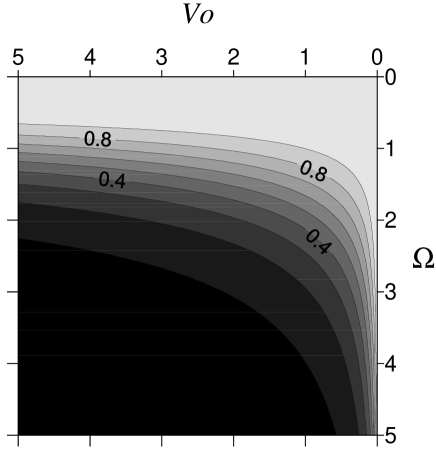
Figure 8: Critical value of the wavenumber $\tilde{k}_{c}$ as function of $Vo\equiv V\Omega^{-2}$ and the frequency $\Omega$. $\tilde{G}_{0}=3.33\cdot 10^{-4}$.

Introduction of the rescaled wavenumber $\tilde{k}=k\sqrt{C/3A}$ and the growth rate $\tilde{\lambda}=\lambda C/\left(3A^{2}\right)$ results in the following expressions for $\tilde{\lambda}$:

$$\tilde{\lambda}=\tilde{k}^{2}\left\{\tilde{G}_{0}-1+\tilde{k}^{2}\left[1+Vf_{r}(\alpha)\right]\right\},$$ (87)

and for the critical wavenumber:

$$\tilde{k}_{c}^{2}=\frac{1-\tilde{G}_{0}}{1+Vf_{r}(\alpha)}.$$ (88)

Here

$$\tilde{G}_{0}=\frac{G_{0}}{3A},\ V=\frac{b^{2}\Omega^{2}}{2C}=\frac{B^{2}\Omega^{2}}{2Ca}$$ (89)

are the rescaled Galileo number and the vibrational parameter, respectively. The Galileo number usually is quite small for thin films. We take $\tilde{G}_{0}=3.3\cdot 10^{-4}$. This corresponds to $A^{\prime}=6\pi\cdot 10^{-21}J$ (value for water) and $\hat{H}_{0}=1000\AA$. Dependence of $\tilde{\lambda}(\tilde{k})$ is shown in Fig. 7 for various values of $\Omega$ and $V$. Clearly, $\tilde{k}_{c}$ decreases with $V$. Moreover, as it is shown in Fig. 8, $k_{c}$ also decreases with growth of $\Omega$. Thus the vibration stabilizes the film. And, stabilization is more pronounced for larger values of $\Omega$.

VIII.2 Weakly nonlinear analysis

Let consider the behavior of perturbations near the stability threshold determined in the previous subsection. For this purpose it is convenient to rescale the time and the coordinate as follows:

$$\tilde{X}=\sqrt{\frac{3A}{C}}X,\ \tilde{T}=\frac{3A^{2}}{C}T.$$ (90)

Substituting these relations into Eqs. (36) one can obtain

$$h_{\tilde{T}} = \left(h^{3}\tilde{\Pi}_{\tilde{X}}-3VQ\right)_{\tilde{X}},$$ (91a)

$$\tilde{\Pi} \equiv \frac{1}{3h^{3}}-h_{\tilde{X}\tilde{X}}+\tilde{G}_{0}h+V{\rm Re}H,$$ (91b)

$$Q = Q_{1}(\gamma)h^{2}h_{\tilde{X}}^{3}+Q_{2}(\gamma)h^{3}h_{\tilde{X}}h_{\tilde{X}\tilde{X}},$$ (91c)

where $Q_{1,2}$ are given by Eqs. (37) and the rescaled parameters defined by Eq. (89) are used. Below we use only the rescaled coordinate and the time. Thus we omit the tildes above $X$ and $T$.

In Sec. VIII.1 it has been shown that the growth rate is real at the stability threshold. Consequently, the branching solution is stationary, i.e. one can omit the left-hand side of the amplitude equation to study direction of branching only. This also allows us to integrate Eq. (91) once. Besides, seeking the solution with fixed wavenumber $\tilde{k}$ we introduce the variable $\zeta=\tilde{k}X$. The surface deflection $h$ now is a $2\pi$-periodic function of $\zeta$, and it solves the following equation:

$$h^{3}\left(\frac{1}{3h^{3}}-\tilde{k}^{2}h_{\zeta\zeta}+\tilde{G}_{0}h+V\tilde{k}^{2}{\rm Re}H\right)_{\zeta}-3V\tilde{k}^{2}Q=const.$$ (92)

Note that $X$ must be replaced with $\zeta$ in the expressions for $Q_{1,2}$ and $H$.

Next, we expand $h$ near the base solution (80) as follows:

$$h=1+\delta h_{1}+\delta^{2}h_{2}+\ldots.$$ (93)

The wavenumber is assumed close to the critical value $k_{0}$, i.e.

$$\tilde{k}=\tilde{k}_{0}+\delta^{2}\tilde{k}_{2}+\ldots.$$ (94)

Substituting these expansions into Eq. (92), we arrive at order zero to

$$\hat{L}h_{1}\equiv(1-\tilde{G}_{0})h_{1}^{\prime}+\tilde{k}_{0}^{2}\left[1+Vf_{r}(\alpha)\right]h_{1}^{\prime\prime\prime}=0,$$ (95)

where the prime denotes the derivative with respect to $\zeta$. Solution of this equation is

$$h_{1}=a\cos\zeta.$$ (96)

The wavenumber is given by the expression

$$\tilde{k}_{0}^{2}=\frac{1-\tilde{G}_{0}}{1+Vf_{r}(\alpha)},$$ (97)

which obviously coincides with Eq. (88). Recall that we are interested in the case $\tilde{G}_{0}<1$ which holds true for the thin film.

The equation at the second order in $\delta$ has the form:

$$\hat{L}h_{2} = 2(h_{1}^{2})^{\prime}+V\tilde{k}_{0}^{2}F_{1}\left(h_{1}h_{1}^{\prime\prime\prime}+3h_{1}^{\prime}h_{1}^{\prime\prime}\right)$$ (98)

$$-3V\tilde{k}_{0}^{2}Q_{2}h_{1}^{\prime}h_{1}^{\prime\prime}.$$

The solution of this equation is

$$h_{2} = C_{1}a^{2}\cos 2\zeta,$$ (99)

$$C_{1} = -\frac{1}{3(1-\tilde{G}_{0})}\left[1+V\tilde{k}_{0}^{2}\left(F_{1}+\frac{3}{4}Q_{2}\right)\right].$$

Hereafter

$$F_{1}=\left(\frac{dF}{dh}\right)_{h=1},\ F_{2}=\left(\frac{d^{2}F}{dh^{2}}\right)_{h=1},\ F\equiv hf_{r}(\alpha h).$$ (100)

At the third order we need only the solvability condition. (We do not present here the corresponding equation for $h_{3}$.) This condition couples the correction to the wavenumber $k_{2}$ to the amplitude of the perturbation $a$, as follows:

$$\tilde{k}_{2}=\frac{\tilde{k}_{0}a^{2}}{2\left(1-\tilde{G}_{0}\right)}\left[\frac{5}{2}-2C_{1}+V\tilde{k}_{0}^{2}\left(\frac{9}{4}Q_{1}+3Q_{2}C_{1}-\frac{3}{4}Q_{2}^{\prime}-\frac{1}{2}C_{1}F_{1}-\frac{1}{8}F_{2}\right)\right].$$ (101)

Our numerical simulations show that the expression in the square brackets is always positive. Thus $\tilde{k}_{2}>0$, i.e. a small amplitude solution exists at $\tilde{k}>\tilde{k}_{0}$. This means that the subcritical bifurcation takes place.

To summarize, the solution emerging at $\tilde{k}=\tilde{k}_{0}$ is unstable and a finite amplitude excitation (probably leading to rupture) is expected.

VIII.3 Nonlinear evolution of perturbations

In this Section we analyze the finite-amplitude deflections of the free surface, starting from stationary solutions $h_{s}$ of the amplitude equation. For this purpose we look for the periodic (with respect to $\zeta$) solutions of Eq. (92).

Due to evident symmetry properties of the solution one can integrate Eq. (92) over half of the period, vanishing all the odd derivatives at $\zeta=0,\pi$. This means that $const.=0$ in Eq. (92). We also have two boundary conditions:

$$h_{s}^{\prime}=0\ {\rm at}\ \zeta=0,\pi.$$ (102)

Besides, the stationary solution conserves the liquid volume:

$$\int_{0}^{\pi}(h_{s}-1)d\zeta=0.$$ (103)

This provides the third boundary condition for the third order ODE, Eq. (92), completing the problem statement.

Figure 9: Unstable stationary solutions computed from Eq. (92) for $\tilde{G}_{0}=3.33\cdot 10^{-4},\ \Omega=0.2$. (a): $\tilde{k}=1.1$, (b): $\tilde{k}=2.2$, (c): $\tilde{k}=4.4$. Dashed, solid, and dash-dotted lines correspond to $V=0,\,50,\,200$.

Figure 10: Minimal (lower branch) and maximal (upper branch) thickness of the film at the corresponding unstable stationary solution. $\tilde{G}_{0}=3.33\cdot 10^{-4}$. (a): $\Omega=0.02$, dashed, solid, and dash-dotted lines correspond to $V=0,\,800,\,5000$ ($\tilde{k}_{0}=0.99998,\,0.9793,\,0.8885$); (b): $\Omega=0.2$, dashed, solid, and dash-dotted lines correspond to $V=0,\,50,\,200$ ($\tilde{k}_{0}=0.99998,\,0.8891,\,0.6968$); (c): $\Omega=2$, dashed, solid, and dash-dotted lines correspond to $V=0,\,8,\,50$ ($\tilde{k}_{0}=0.99998,\,0.5287,\,0.2418$). Arrows show boundaries of domains of attraction.

The shooting method is applied to numerically integrate this boundary value problem. Some results are presented in Figs. 9 and 10. It is clearly seen that only the subcritical (and, consequently, unstable) solution branch is present, i.e. there is no bifurcation except the inverse pitchfork bifurcation studied in Sec. VIII.2. Therefore, the lower branches in Fig. 10 are the boundaries of domains of attraction: the initial perturbation with $min[h(\zeta,T=0)]>h_{m}$ decays and the free surface becomes flat, while in the opposite case the free surface is attracted to the solid, which leads to rupture. These predictions are in good agreement with the results of the numerical simulation of Eqs. (91), as shown in Fig. 11.

Figure 11: Evolution of the minimum film thickness, as given by direct numerical computation of Eq. (36). Unstable stationary solutions with small perturbation of the free surface $\delta_{h}$ were chosen for the initial condition. $\tilde{G}_{0}=3.33\cdot 10^{-4},\ \tilde{k}=1.1,\ \Omega=0.02,\ V=800$. $\delta_{h}=0.009,\,0.002,\,0,\,-0.002,\,-0.01$ (dash-double-dotted, dash-dotted, solid, dotted, and dashed lines, respectively).

The upper branches in Figs. 10 are of importance for the stability of the oscillatory flow (see Sec. VII). Indeed, Eq. (64) requires the maximal value of the surface deviation $h_{0}$, which can be extracted from Fig. 10.

It is important to point out that the increase of the vibration amplitude amplifies the film stability: at fixed $\tilde{k}$ and with $\Omega$ increasing, the initial deviation of the flat surface decays at larger values of $V$. The only exception is provided by $\Omega=2$. In this case $h_{m}$ is nonmonotonic function of $V$ starting from certain value of $\tilde{k}$. Also it is interesting that the maximal deviation of the surface decreases with growth of $V$: the surface tends to become flat as it is shown in Fig. 9. In some sense this tendency is reminiscent of the known averaged behavior LChbook ; LChMcgr : the free surface/interface tries to orient normally to the vibration axis. But it is necessary to keep in mind that the surfaces shown in Fig. 9 correspond to unstable states.

IX Summary

In this paper the impacts of the vertical vibration on the dynamics of the thin liquid film are analyzed. The set of equations governing the averaged dynamics of the fluid flow and the nonlinear, fourth-order amplitude equation (36) [or (49) in 3D case] describing the averaged evolution of the film thickness are obtained in the lubrication approximation.

We use the paradoxical scaling (at least at the first glance), assuming (i) the vibration period is comparable to the characteristic time of the momentum relaxation across the layer and (ii) the vibration amplitude is large in comparison with the mean layer thickness. The first condition (termed “moderate frequency” or “finite frequency”) allows us to consider ultrathin liquid layers within the framework of the averaging method. The second condition warrants that the impact of the vibration is not vanishingly small. Using the results from Refs. Mancebo ; Straatman ; Singer we prove that these assumptions do not necessarily lead to the parametric instability.

Indeed, we show that the stability problem for the pulsatile flow can be separated into the problems for the deformable and non-deformable modes. The former problem reduces to the analysis of Faraday instability, while the latter problem reduces to the stability analysis of the oscillatory Poiseuille flow. Analyzing well known results obtained for these two problems we deduce that there exists a window of stability: below certain threshold intensity of the vibration [Eqs. (64) and (79)] the pulsatile flow is stable, while the averaged effects are well pronounced.

The analyses of the averaged dynamics of the thin film demonstrate the strong stabilizing impact of the vibration. First, the vibration damps the short-wavelength instability. In other words, it decreases the critical cut-off wavenumber $k_{c}$, such that instability occurs at $k<k_{c}$ only [see Eqs. (83), (85) and Figs. 7 and  8]. In this sense the vibration acts in a way similar to the surface tension. Therefore, in order to prevent a longwave instability one can use a cavity of horizontal size $L<L_{c}\sim k_{c}^{-1}$, which is larger in presence of the vibration. Second, the vibration augments the domain of attraction of the flat undeformed surface, i.e. larger initial surface deflections decay (see Fig. 10) or, in other words, larger initial distortions of a flat surface are admissible without occurrence of dewetting.

Thus, the vertical vibration of moderate frequency is the effective method of control of the thin film instability. This is especially important since the standard (high-frequency) approximation cannot be applied to thin films.

X Acknowledgments

S. S. was partially supported by the Fund “Perm Hydrodynamics”. A. A. A. acknowledges CRDF for the financial support within the framework of grant Y3-MP-09-01.

Appendix A Reduction of pulsatile flow to the oscillatory Poiseuille flow

In this section we show that the pulsatile flow given by Eqs. (20) and (22) can be reduced to the well- known oscillatory Poiseuille flow. Such a transformation is useful for the stability analysis carried out in Sec. VII.2. Throughout this section we omit the tildes over the velocity and the pressure field, with the understanding that only the oscillatory components are involved.

In order to obtain the oscillatory Poiseuille flow we return to the unscaled coordinates $x$ and $z$, setting locally

$$h=h_{0}+O(\epsilon),\ h_{X}=const+O(\epsilon).$$ (104)

These equations mean that the layer thickness changes slowly with $x$. Thus one can assume the constant thickness $h_{0}$. In view of the scaling (12b) and Eqs. (20) and (22) the longitudinal pressure gradient is $b\Omega h_{X}\cos\tau$. Thus the pressure gradient is spatially uniform but oscillates in time. This means that some kind of the so-called oscillatory Poiseuille flow is under consideration.

Neglecting $h_{XX}$ according to Eq. (104) we arrive at the following expressions for the amplitudes of pulsations

$$I = ih_{X}\left(1-\frac{\cos\alpha(h_{0}-z)}{\cos\alpha h_{0}}\right),$$ (105a)

$$K = ih_{X}^{2}\frac{1-\cos\alpha Z}{\cos^{2}\alpha h_{0}},\ H=h_{X}^{2}\tan^{2}\alpha h_{0},$$ (105b)

which along with the scalings (12b) and (13) gives:

$$u = b\Omega h_{X}{\rm Re}\left[i\left(1-\frac{\cos\alpha(h_{0}-z)}{\cos\alpha h_{0}}\right)e^{i\tau}\right],$$ (106)

$$w = O(\epsilon),\ h-h_{0}=O(\epsilon).$$ (107)

Thus this case corresponds to oscillatory 1D flow in a locally flat layer under the spatially uniform longitudinal gradient of pressure. Note that the second relation in Eqs. (107) justifies the first assumption in Eqs. (104).

Separating the real and imaginary parts in Eq. (106) we arrive at the following expressions for the $x$-component of the pulsation velocity:

$$u = -b\Omega h_{X}\left\{\left[1-\frac{a_{S}(h_{0})a_{S}(z)+b_{S}(h_{0})b_{S}(z)}{a_{S}^{2}(h_{0})+b_{S}^{2}(h_{0})}\right]\sin\tau-\frac{a_{S}(h_{0})b_{S}(z)-a_{S}(z)b_{S}(h_{0})}{a_{S}^{2}(h_{0})+b_{S}^{2}(h_{0})}\cos\tau\right\},$$ (108)

$$a_{S}(z) \equiv \cos\alpha_{r}z\cosh\alpha_{r}z,\ b_{S}(z)\equiv\sin\alpha_{r}z\sinh\alpha_{r}z,\ \alpha_{r}=\sqrt{\Omega/2}.$$

Such flow, but in a gap between two rigid boundaries, is well studied – see, for instance, the recent papers by Singer et al. Singer and Straatman et al. Straatman , who address the stability problem for the flow. (Usually the modulated Poiseuille flow is considered, i.e. the pressure gradient oscillates about a non-zero mean value.)

Due to symmetry the oscillatory Poiseuille flows in a layer with the free nondeformable surface at $z=h_{0}$ and in a layer with the upper rigid wall at $z=2h_{0}$ are identical. Indeed, in the latter case in the plane of symmetry $z=h_{0}$ the “no-stress” condition $u_{z}=0$ is obviously held.

Thus, introducing variable $y_{S}=z-h_{0}$ in Eq. (108) we obtain the velocity profile of the oscillatory Poiseuille flow [cf. oscillatory part of Eq. (2.2) in Ref. Singer ].

Appendix B Solution of the set of averaged equations

Solution of the problem for the averaged fields can be represented as the sum of two solutions. The first one is conventional (see, for example, Ref. Oron ); we mark it by the subscript “$c$”:

$$p_{c} \equiv \Pi-G_{0}Z$$ (109a)

$$= \phi-Ch_{XX}+G_{0}(h-Z)+\frac{b^{2}\Omega^{2}}{2}{\rm Re}H,$$

$$U_{c} = \frac{1}{2}Z(Z-2h)\Pi_{X},$$ (109b)

$$W_{c} = -\frac{1}{3}\left[Z^{2}(Z-3h)\Pi_{X}\right]_{X}.$$ (109c)

Note that this solution leads to the first term in the evolution equation for the film thickness, Eq. (36). This part of the solution coincides with Eqs. (2.47) in Ref. Oron up to the averaged correction to the pressure field.

The second part is the solution of the nonhomogeneous boundary value problem with the remaining vibration-generated terms at the right-hand sides. Using subscript “$v$” for this part of solution, we rewrite it in the following form:

$$p_{v}=0,\ U_{v}=\frac{1}{2}b^{2}\Omega^{2}U^{(v)},\ W_{v}=\frac{1}{2}b^{2}\Omega^{2}W^{(v)},$$ (110)

where $U^{(v)}$ and $W^{(v)}$ solve the following boundary value problem:

$$U^{(v)}_{ZZ} = {\rm Re}\left(I^{*}I_{X}+K^{*}I_{Z}\right),\ W^{(v)}_{Z}=-U_{X}^{(v)},$$ (111a)

$$U^{(v)} = W^{(v)}=0\ {\rm at}\ Z=0,$$ (111b)

$$U_{Z}^{(v)} = -\Omega^{-1}{\rm Re}\left(I_{ZZ}^{*}H\right)\ {\rm at}\ Z=h.$$ (111c)

This set of equations can be easily integrated. First,

$$U_{Z}^{(v)}=-\Omega^{-1}{\rm Re}\left[I_{ZZ}^{*}(h)H\right]-\int_{Z}^{h}{\rm Re}\left(I^{*}I_{X}+K^{*}I_{Z}\right)dZ.$$ (112)

Accounting for Eq. (21) of the pulsatile motion and integrating by parts, one can rewrite the last expression as

$$U_{Z}^{(v)}=-h_{X}{\rm Re}H+{\rm Re}\left(I^{*}K\right)-\partial_{X}\int_{Z}^{h}|I|^{2}dZ.$$ (113)

After one more integration we arrive at the following solution:

$$U^{(v)} = -Zh_{X}{\rm Re}H+\int_{0}^{Z}{\rm Re}\left(I^{*}K\right)dZ$$ (114)

$$-\partial_{X}\int_{0}^{Z}d\zeta\int_{\zeta}^{h}|I(X,\xi)|^{2}d\xi.$$

Evaluation of these integrals leads to the cumbersome formulas, which we do not present here.

We also do not present the expression for $W^{(v)}$, as it is not needed in order to obtain the evolution equation for film thickness $h$. Indeed, this part of the solution results in the term

$$-\partial_{X}\int_{0}^{h}U^{(v)}dZ-\Omega^{-1}{\rm Re}\{I^{*}H\}$$ (115)

at the right-hand side of such an equation. This term translates to the term $Q(h)$ in Eq. (36).

References

- (1) U. Thiele, M. Mertig, and W. Pompe, Phys. Rev. Lett. 80, 2869 (1998).
- (2) M. P. Ida and M. J. Miksis, SIAM J. Appl. Math. 58, 456 (1998).
- (3) A. Ghatak, R. Khanna, and A. Sharma, J. Colloid Interface Sci. 212 483 (1999).
- (4) L. M. Pismen, B. Y. Rubinstein, and I. Bazhlekov, Phys. Fluids 12, 480 (2000).
- (5) T. P. Witelski and A. J. Bernoff, Physica D 147, 155 (2000).
- (6) R. Seemann, S. Herminghaus, and K. Jacobs, Phys. Rev. Lett. 87, 196101 (2001).
- (7) A. A. Golovin, B. Y. Rubinstein, and L. M. Pismen, Langmuir 17, 3930 (2001).
- (8) K. B. Glasner and T. P. Witelski, Phys. Rev. E 67, 016302 (2003).
- (9) M. Bestehorn, A. Pototsky, and U. Thiele, Eur. Phys. J. B 33, 457 (2003).
- (10) T. Yi and H. Wong, J. Colloid and Interface Sci. 313, 579 (2007).
- (11) A. Oron, S. H. Davis, and S. G. Bankoff, Rev. Mod. Phys. 69, 931 (1997).
- (12) R. Seemann, S. Herminghaus, and K. Jacobs, J. Phys.: Condensed Matter 13, 4925 (2001).
- (13) G. H. Wolf, Z. Phys. 227, 299 (1969).
- (14) G. H. Wolf, Phys. Rev. Lett. 24, 444 (1970).
- (15) V. Kozlov, A. Ivanova, and P. Evesque, Europhys. Lett. 42, 413 (1998).
- (16) A.A. Ivanova, V. G. Kozlov, and P. Evesque, Izv. RAN. Mekh. Zhidk i Gaza 3, 28 (2001) [Fluid Dynamics 36, 362 (2001)].
- (17) G. Z. Gershuni and D. V. Lyubimov, Thermal Vibrational Convection (Wiley, New York, 1998).
- (18) D. V. Lyubimov, T. P. Lyubimova, and A. A. Cherepanov, Dynamics of interfaces in vibration fields (Fizmatlit, Moscow, 2004) (in Russian).
- (19) V. Lapuerta, F. J. Mancebo, and J. M. Vega, Phys. Rev. E 64, 016318.
- (20) U. Thiele, J. M. Vega, and E. Knobloch, J. Fluid Mech. 546, 61 (2006).
- (21) M.V. Khenner, D.V. Lyubimov, T.S. Belozerova, and B. Roux, Europ. J. Mech. B/Fluids 18 1085 (1999).
- (22) H. Schlichting, Boundary-Layer Theory, 8th Ed. (Springer, 2000).
- (23) J. A. Sanders and F. Verhulst, Averaging methods in nonlinear dynamical systems (Springer-Verlag, New York, 1985).
- (24) A. H. Nayfeh, Perturbaton methods (Wiley, New York, 1973).
- (25) P. L. Kapitza, Zh. Eksp. Teor. Fiz. 21, 588 (1951) (in Russian).
- (26) I. I. Blekhman, Vibrational Mechanics: Nonlinear Dynamic Effects, General Approach, Applications (World Scientific, Singapore, 2000).
- (27) Z. C. Feng and Y. H. Su, Phys. Fluids 9, 519 (1997).
- (28) Z. Zapryanov and S. Tabakova, Dynamics of Bubbles, Drops and Rigid Particles (Kluwer Academic Publishers, Dordrecht, 1999).
- (29) P. Evesque and J. Rajchenbach, Phys. Rev. Lett. 62, 44 (1989).
- (30) A. V. Straube, D. V. Lyubimov, and S. V. Shklyaev, Phys. Fluids 18, 053303 (2006).
- (31) D. V. Lyubimov and G. A. Sedelnikov, Izv. RAN. Mekh. Zhidk. i Gaza 1, 6 (2006) [Fluid Dynamics 41, 3 (2006)].
- (32) A. A. Cherepanov, in Some problems of stability of a liquid surface, Sverdlovsk, USSR, 1984 (in Russian).
- (33) M. Faraday, Phylos. Trans. R. Soc. London 121, 299 (1831).
- (34) T. B. Benjamin and F. Ursell, Proc. Roy. Soc. A 255, 505 (1954).
- (35) K. Kumar and L. S. Tuckerman, J. Fluid Mech. 279, 49 (1994).
- (36) D. V. Lyubimov and A. A. Cherepanov, in Some problems of stability of a liquid surface, Sverdlovsk, USSR, 1984 (in Russian).
- (37) F. J. Mancebo and J. M. Vega, J. Fluid Mech. 467, 307 (2002).
- (38) I. E. Dzyaloshinskii, E. M. Lifshitz, and L. P. Pitaevskii, Zh. Eksp. Theor. Fiz. 37, 229 (1959) [Sov. Phys. JETP 10, 161 (1960)].
- (39) C. C. Mei and L. F. Liu, J. Fluid Mech. 59, 239 (1973).
- (40) B. A. Singer, J. H. Ferziger, and H. L. Reed, J. Fluid Mech. 208, 45 (1989).
- (41) A. G. Straatman, R. E. Khayat, E. Haj-Qasem, and D. A. Steinman, Phys. Fluids 14, 1938 (2002).
- (42) J. W. S. Rayleigh, The Theory of Sound, 2nd edition (Dover Publ., New York, 1945).
- (43) H. B. Squire, Proc. R. Soc. London, Ser. A 142, 621 (1933).
- (44) S. H. Davis, Annu. Rev. Fluid Mech. 7, 57 (1976).
- (45) C. von Kerczek and S. H. Davis, J. Fluid Mech. 62, 753 (1974).
- (46) S. A. Orszag, J. Fluid Mech. 50, 689 (1971).
- (47) D. V. Lyubimov, A. A. Cherepanov, T. P. Lyubimova, and B. Roux, Micrograv. Quart. 6, 69 (1996).