Distances in
random Apollonian network structures

Abstract

In this paper, we study the distribution of distances in random Apollonian network structures (RANS), a family of graphs which has a one-to-one correspondence with planar ternary trees. Using multivariate generating functions that express all information on distances, and singularity analysis for evaluating the coefficients of these functions, we describe the distribution of distances to an outermost vertex, and show that the average value of the distance between any pair of vertices in a RANS of order $n$ is asymptotically $\sqrt{n}$.

1 Introduction

Many graph models have been recently introduced for representing the structure and dynamics of real-life networks (see e.g. [3]). Their adequacy to data can be measured by comparing some properties of graphs, especially the degree distribution of the vertices, which is related to scale-free properties, and properties related to the “small world” effect, such as distance between pairs of vertices and grouping in clusters.

The random Apollonian networks (RAN) proposed by [4] provides a very interesting model, with a power-law degree distribution, a mean distance of logarithmic order and a large clustering coefficient. We introduced in [1] a modified version, random Apollonian network structures (RANS), which preserves the interesting properties of real graphs concerning degree distribution (a power-law with an exponential cut-off) and large clustering. This paper is devoted to the analysis of distances in RANS, which is showed to be of square root order: we first characterize the distances from one special vertex to all the other vertices of the graph, and then work on the distances between pairs of vertices.

A RANS can be seen as a certain type of triangulation of a triangle, and the study of RANS relies on the bijection with planar ternary trees (see figure 1). From this bijection we can express the enumerative generating function for RANS, and use multivariate functions for marking several distance parameters. Moreover the asymptotic values of the quantities under consideration can be dealt with using singularity analysis (according to methods developed in [2]).

We are interested in two types of parameters measuring distance, and develop two methods to handle them. We first attack the distances between a special vertex (an outermost vertex A of the RANS) and all the other vertices. The method is built on computing a generating function with infinitely many variables, that contains all informations concerning distances from A to the other vertices. Distribution analysis is based on the study of partial derivatives of this multivariate series, which correspond to the series counting the number of vertices at a certain distance from A. These series all express in terms of the generating function for RANS and asymptotic analysis gives a distribution with a mean value of order $\sqrt{3\pi n}/11$.

The second study addresses the total distance between all pairs of vertices. We exhibit a generating function in four variables that expresses simultaneously distances from one, two or three outermost vertices. This generating function has a nice recursive definition, due to the symmetries of the problem. It contains all information to compute the total distance between pairs of vertices. Geometrical considerations splits this total distance in two parts, depending on whether a path between two vertices spans over disjoints sub-RANS or not. The resulting mean distance between two vertices is of order $2\sqrt{3\pi n}/11$.

This paper divides in four sections: this introduction, followed by a section that recalls the definition of random Apollonian network structures, the bijection with ternary trees, and the result for degree distribution. Section 3 describes the distribution of distances from an outermost vertex and section 4 is dedicated to the study of the total distance between all pairs of vertices.

2 Random Apollonian network structures

The recursive definition of RANS shows a one-to-one correspondence with ternary trees. The degree distribution, which is a power law with an exponential cut-off, was studied in [1] by considering bivariate series marking the corresponding parameter in trees.

2.1 Bijection with ternary trees

A random Apollonian network structure (RANS) $R$ is recursively defined as: either an empty triangle or a triangle $T$ split in three parts, by placing a vertex $v$ inside $T$ and connect it to the three vertices of the triangle; each sub-triangle being substituted by a RANS (see figure 1).

The vertices of $T$ will be called the outermost vertices of $R$ (noted $\mathcal{O}(R)$); and vertex $v$ will be called the center of $R$. We will note $\mathcal{R}$ the class of all RANS.

The order of the empty RANS is zero and the order of a non-empty RANS is one plus the sum of the orders of the three sub-RANS.

Proposition 2.1.

[1] There is a bijection between random Apollonian network structures of order $N$ and rooted plane ternary trees of size $N$ (with $N$ internal nodes).

In planar ternary trees, the linear ordering of siblings is relevant. This order is carried over to triangles: naming $\{O_{1},O_{2},O_{3}\}$ the vertices of $\mathcal{O}(R)$, imposes a linear ordering on the sub-RANS ($\{S_{1},S_{2},S_{3}\}=\mathcal{S}(R)$): $S_{i}$ will be the one not containing $O_{i}$. Recursively replacing the missing outermost vertex by the center of $R$ preserves the order in sub-RANS.

The generating function for ternary trees $T(z)=\sum T_{N}z^{N}$ satisfies the functional equation $T(z)=1+zT^{3}(z)$, whose solution can be analysed locally through singularity analysis. $T(z)$ has radius of convergence $\rho=4/27$ and singular value $\tau=3/2$; and the singular expansion of $T(z)$ near $\rho$ is

$$T(z)=\frac{3}{2}-\frac{\sqrt{3}}{2}\sqrt{1-z/\rho}+\frac{2}{3}(1-z/\rho)-\frac{35\sqrt{3}}{108}(1-z/\rho)^{3/2}+O\left((1-z/\rho)^{5/2}\right).$$ (1)

Thus the asymptotic form of the coefficients: $T_{N}\sim c\rho^{-N}N^{-3/2}$, with $c=\sqrt{3}/4\sqrt{\pi}$.

The derivative $T^{\prime}(z)=\frac{T^{3}(z)}{1-3zT^{2}(z)}$ will also appear in the computations below. The leading term in its singular expansion is $\frac{\sqrt{3}}{4\rho}(1-{z}/{\rho})^{-1/2}$, thus a coefficient $T^{\prime}_{N}$ of asymptotic order $\frac{27\sqrt{3}}{16\sqrt{\pi}}\rho^{-N}N^{-1/2}$.

2.2 Degree distribution

The degree distribution in random Apollonian network structures follows a power law with an exponential cutoff. This is obtained by analysing the degree of the center of a RANS (which corresponds to the size of a binary subtree at the root of the corresponding ternary tree), and propagating this study to the whole of the sub-RANS.

The bivariate generating function marking the degree of the center is $D_{g}(z,u)=zu^{3}T^{3}(z,u)$, where $T(z,u)$ is the bivariate generating function for ternary trees with $u$ marking the size of the underlying binary subtree, which is also the degree of an outermost vertex:

$$T(z,u)=1+uzT(z)T^{2}(z,u).$$ (2)

Theorem 2.2.

[1] The degree distribution in random Apollonian network structures follows a power law with an exponential cutoff: $\Pr(D_{g}=k)\sim C\,\beta^{k}\ k^{-3/2}$, with $\beta=\frac{8}{9}$.

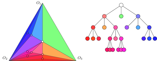
Figure 1: A random Apollonian network and its corresponding ternary tree

3 Distance from an outermost vertex

This section is devoted to computing the distribution of the distances from a fixed specific outermost vertex. We introduce a generating function with infinitely many variables, each variable $u_{i}$ marking the number of vertices at distance $i$ from the outermost vertex. Relying on the symmetries of the problem and the recursive nature of RANS, we are able to express and study this generating function.

The interest of this analysis is not only to find, with a different method, some results of the following section; but moreover this study can be adapted to compute the distribution of distances to any distinguished vertex in a RANS, which may be considered as a more realistic parameter.

3.1 Multivariate generating function

Due to the recursive nature of RANS, we often have to consider a RANS $R$ as having an environment, that is a bigger RANS containing $R$. Given a RANS $R$, the distance of any of its vertices to a vertex $v$ in the environment of $R$ is determined by the three distances of the elements of $\mathcal{O}(R)$ to $v$.

Since the outermost vertices of $R$ form a clique, their distances to any vertex cannot differ by more than one. This observation allows us to reduce our study to a few cases. First we work modulo a translation and restrict ourselves to the case when the three distances to $\mathcal{O}(R)$ are either $1$ or $0$. Second we can work modulo a permutation and restrict ourselves to only three cases: $(0,1,1)$, $(0,0,1)$ and $(0,0,0)$, illustrated in figure 2. These three cases actually correspond to labelling the internal vertices of $R$ by their distances either to one (out of three), or to two (out of three) or to all three outermost vertices.

• The $\delta_{(}1)$-labeling of $R\in\mathcal{R}$ consists in putting on each vertex a label corresponding to its distance from $O_{1}(R)$ (or equivalently to one of any $O_{i}(R)$):

  • the outermost vertices $O_{1},O_{2},O_{3}$ respectively receive labels $0$, $1$ and $1$;

  • the center of $R^{\prime}\in\mathcal{S}(R)$ is labeled by 1 plus the minimum of the labels of $\mathcal{O}(R^{\prime})$.

• Let’s define the type of $R\in\mathcal{R}$ as the set of labels of $\mathcal{O}(R)$. We say that

  • two RANS types are equivalent iff they have the same type up to a permutation.

  • two RANS types are translated by $\theta$ iff their labellings are the same up to a translation $\theta$.

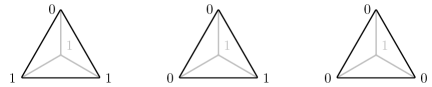
Figure 2: RANS of type $(0,1,1),(0,0,1),(0,0,0)$ and their sub-RANS.

In a RANS $R$ of type $(0,1,1)$ the center gets label 1. Thus $R$ is equivalent to $S_{2}(R)$ and $S_{3}(R)$, but it is not equivalent to $S_{1}(R)$, which is of type $(1,1,1)$: if a vertex is at distance $d$ from $O_{1}(S_{1}(R))$, its distance from $O_{1}(R)$ is $d+1$.

This remark leads to the bivariate generating function for RANS marked with vertices at distance 1 from $O_{1}(R)$:

$$T_{1}(z,u_{1})=1+{\color[rgb]{0.438,0.438,0.438}zu_{1}}{\color[rgb]{0,.5,.5}T_{1}^{2}(z,u_{1})}{\color[rgb]{.5,0,.5}T(z)}.$$ (3)

This follows the recursive definition of RANS, noticing first that the center is at distance $1$ from $O_{1}(R)$ and second that the configuration is the same in $S_{2}(R)$ and $S_{3}(R)$, whereas in $S_{1}(R)$ there is no vertex at distance $1$ from $O_{1}(R)$. Note that (3) is obviously the same generating function as (2), the degree of a vertex being exactly the number of vertices at distance $1$ from this vertex.

The problem of marking both vertices at distance 1 and 2 from $O_{1}(R)$ is treated in the same way: the configuration of $R$, of type $(0,1,1)$, recursively occurs in $S_{2}(R)$ and $S_{3}(R)$, which are of the same type. But the case of $S_{1}(R)$, of type $(1,1,1)$, is a little more tricky and requires a deeper decomposition. If $S_{1}(R)$ is not empty, its center is at distance 2 from $O_{1}(R)$, and its three sub-RANS $\mathcal{S}(S_{1}(R))$ are equivalent, of type $(1,1,2)$: either they are empty, or their center is at distance 2 from $O_{1}(R)$, one sub-RANS is of type $(1,1,2)$, equivalent to $\mathcal{S}(S_{1}(R))$ and the two others are of type $(1,2,2)$, translated by 1 with $R$, which means that the number of their vertices at distance 2 from $O_{1}(R)$ in is the same as the number of vertices at distance 1 from $O_{1}(R)$ in $R$.

This decomposition leads to the following functional equations, with $u_{j}$ marking vertices at distance $j$ from $O_{1}(R)$:

$$T_{2}(z,u_{1},u_{2}) =1+zu_{1}{\color[rgb]{0,.5,.5}T_{2}^{2}(z,u_{1},u_{2})}{\color[rgb]{.5,0,.5}F(z,u_{1},u_{2})}$$

$$F(z,u_{1},u_{2}) =1+{\color[rgb]{0.438,0.438,0.438}zu_{2}}{\color[rgb]{.75,0,.25}G^{3}(z,u_{1},u_{2})},$$

$$G(z,u_{1},u_{2}) =1+{\color[rgb]{0.438,0.438,0.438}zu_{2}}{\color[rgb]{.75,0,.25}G(z,u_{1},u_{2})}{\color[rgb]{0,0.3,0}T_{1}^{2}(z,u_{2})}.$$

It is easy to show that the same equations hold for $d\geq 3$, when considering multivariate generating functions $T(z,u_{1},u_{2},\ldots,u_{d})$, with $u_{j}$ marking vertices at distance $j$ from $O_{1}(R)$, and we get the following result.

Proposition 3.1.

Let $r_{n,k_{1},\ldots,k_{d}}$ be the number of RANS of order $n$ with $k_{j}$ vertices at distance $j$ from $O_{1}$. Then $r_{n,k_{1},\ldots,k_{d}}$ is the coefficient of $u_{1}^{k_{1}}u_{2}^{k_{2}}\ldots u_{d}^{k_{d}}z^{n}$ in the multivariate series $T_{d}(z,u_{1},\ldots,u_{d})$, where the series $T_{d}$ satisfy the recurrence relations:

$$T_{1}(z,u_{1})=1+zu_{1}T_{1}^{2}(z,u_{1})T_{0}(z)\qquad\hbox{with}\qquad T_{0}(z)=T(z)\\$$

and for $d\geq 2$,

$$T_{d}(z,u_{1},\ldots,u_{d})=1+zu_{1}T_{d}^{2}(z,u_{1},\ldots,u_{d})\left(1+zu_{2}\,\frac{1}{(1-zu_{2}T_{d-1}^{2}(z,u_{2},\ldots,u_{d-1}))^{3}}\right).$$

The sequence $T_{d}(z,u_{1},\ldots,u_{d})$ converges to a function $T_{\infty}(z,u_{1},\ldots,u_{i},\ldots)$ which contains all information concerning distances from vertex $O_{1}$:

• The enumerative series for the number of vertices at distance $i$ from $O_{1}$, over all RANS, is

  $$D_{i}(z)=\left.\frac{\partial}{\partial u_{i}}T_{\infty}(z,u_{1},\ldots,u_{i},\ldots)\right|_{u_{j}=1,\forall j}=\sum_{n}k_{i}\,r_{n,k_{i}}z^{n}.$$

• The asymptotic of the total distance from $O_{1}$ expresses as

  $$\left.\frac{\partial}{\partial u}D(z,u)\right|_{u=1},\qquad\text{where }D(z,u)=\sum_{i=1}^{\infty}D_{i}(z)u^{i}.$$

The aim of the next paragraph is to evaluate these quantities.

3.2 Distribution analysis

Generating functions counting the number of vertices at distance $i$ from $O_{1}$ express as rational functions in $z$ and $T(z)$, and have a singular behaviour similar to $T(z)$: radius of convergence $\rho$, and singular expansion of the square-root type.

Lemma 3.2.

The sequence of enumerative series for the number of vertices at distance $i$ from $O_{1}$ is:

$$D_{1}(z) ={zT^{3}(z)}/{(1-2zT^{2}(z))},$$

$$D_{2}(z) =H(z,T(z))\times{(1+2z^{2}T^{4}(z))}/(6zT(z)(1-2zT^{2}(z)))$$

$$\hbox{and for }\,\,i\geq 2\qquad D_{i+1}(z) =H^{i-1}(z,T(z))\times D_{2}(z),$$

where $H(z,T(z))$ is a rational function in $z$ and $T(z)$, that has radius of convergence $\rho=4/27$, and a singular expansion $H(z)=1-\frac{11}{\sqrt{3}}\sqrt{1-z/\rho}+\frac{2}{3}(1-z/\rho)+(1-z/\rho)^{3/2}+O((1-z/\rho)^{2})$.

Proof.

From (3.1), it is easy to compute the expressions of $D_{1}(z)$ and $D_{2}(z)$, and show that $D_{i+1}(z)=H(z,T(z))\times D_{i}(z)$, with $H(z,T(z))=6z^{2}(T(z)-1)T(z)/(1-3z-zT(z)-zT^{2}(z)+2z^{2}T^{2}(z))$. The singular expansion comes from expressing $z$ as $(T(z)-1)/T^{3}(z)$ and plugging in $H$ the singular expansion (1) of $T(z)$. A full expansion of $T(z)$ yields a full expansion for $H(z)$, the first terms of which are given in the lemma. ∎

The full singular expansion of $D_{i}(z)$ can be derived from its expression in terms of $H$ and $D_{2}$. Thus the proportion of vertices at distance $i$ from $O_{1}$, that is $\frac{1}{nT_{n}}[z^{n}]D_{i}(z)$ can be evaluated. We have no closed form to express these quantities (it is work in progress), but plotting from experimental results obtained on a sample of randomly generated RANS, shows that the distances from $O_{1}$ follow the distribution shown in figure 3.

Figure 3: Distances from $O_{1}$. The points represent the experimental data on RANS of orders 1000–1400.

The average distance from $O_{1}$ is also obtainable by derivation of $D(z,u)=\sum D_{i}(z)u^{i}$. From lemma 3.2 there is a closed form for $D(z,u)$, and derivation leads (fortunately) to the same series as the one obtained for $\Delta_{(}1)(z)$, in section 4.1.

This series has a singular expansion around $\rho$ with first term $\frac{3}{44}(1-z/\rho)^{-2}$, so for the mean distance

$$\frac{1}{nT_{n}}[z^{n}]\left.\frac{\partial}{\partial u}D(z,u)\right|_{u=1}=\frac{\sqrt{3\pi n}}{11}\left(1+O(\frac{1}{n})\right).$$

We thus conclude this section with the following proposition:

Proposition 3.3.

In a RANS of order $n$, the average distance from $O_{1}$ is of order $c\sqrt{n}$, with $c=\sqrt{3\pi}/11$.

4 Total distance between pairs of vertices

Figure 4: All possible configurations for pairs of vertices in $R\in\mathcal{R}$. For each pair in $\mathcal{C}(R)$ we can always find a unique sub-RANS of $R$ such that the two vertices are in one of configurations 2, 4 or 7. The other cases reduce to one of these: case 1 reduces to 2 by looking at the RANS containing $R$, case 3 leads to 2, 3 or 4 by looking in the sub-RANS containing the two vertices, and such is also the case for case 5. Case 6 is amenable to any of 5, 6 or 7 by looking at the sub-RANS containing the two vertices.

In this section, we are interested in computing the total distance of every pair of vertices in a RANS of order $n$, and will show that the mean value of this quantity is still of order $\sqrt{n}$.

We call $\mathcal{C}(R)$ the set of pairs of vertices (we call pair a set of size two) in $R\in\mathcal{R}$, excluding pairs where both vertices are in $\mathcal{O}(R)$.

The enumerative generating function for the total distance between pairs in $\mathcal{C}(R)$ is

$$G(z)=\sum_{R\in\mathcal{R}}\sum_{(v,w)\in\mathcal{C}(R)}dist(v,w)\,\,z^{|R|}.$$

$\mathcal{C}(R)$ splits into two parts

• the pairs $(v,w)$ such that they are both internal vertices of the smallest sub-RANS of $R$ that contains both of them, corresponding to case $7$ in figure 4.

  We will note them $\text{Inter}(R)$ and their contribution to the total distance will be called interdistance.

• the others, which can also be defined as the pairs $(v,w)$ such that there exists a sub-RANS $S$ of $R$ with $v$ an outermost vertex of $S$ and $w$ an internal vertex of $S$, corresponding to cases $2$, $3$ and $4$ in figure 4.

  We will note them $\text{Intra}(R)$ and their contribution to the total distance will be called intradistance.

Remark: $\mathcal{C}(R)$ has $n(n-1)/2+3n$ elements: each pair of internal vertices is counted only once, and the $3n$ term takes into account all pairs made of one internal vertex and one outermost vertex. Among all these pairs, an amount of order $n\sqrt{n}$ belongs to $\text{Intra}(R)$ and the rest is in $\text{Inter}(R)$. As we will show, the total distance of pairs in $\text{Intra}(R)$ is of order $n^{2}$ and the total distance of pairs in $\text{Inter}(R)$ is of order $n^{2}\sqrt{n}$. We can thus say that the interdistance gives the dominant term of the total distance in RANS, which is of order $\sqrt{n}$.

We introduce in the following subsection a new generating function which serves as a basis for the computations of all the quantities that are needed. Then we calculate the intradistance followed by the interdistance. Putting everything together gives the following result.

Theorem 4.1.

The mean distance in a RANS of order $n$ is asymptotically equivalent to $C\sqrt{n}$, with $C=\sqrt{3\pi}/22$.

4.1 Topological generating function

Given $R\in\mathcal{R}$, the distances of inner vertices to $\mathcal{O}(R)$ are denoted by the three following parameters:

$$\Delta_{(}1)(R)=\sum_{x\in R}d(x,O_{1}(R)),\>\Delta_{(}2)(R)=\sum_{x\in R}d(x,\{O_{1}(R),O_{2}(R)\})\>\text{and}\>\Delta_{(}3)(R)=\sum_{x\in R}d(x,\mathcal{O}(R)).$$

Notice that $\Delta_{(}1)(R)$ is the sum of all the labels in the $\delta_{(}1)$-labeling of $R$, based on RANS of type $(0,1,1)$ —see (3.1). Similarly, $\Delta_{(}2)(R)$ is the sum of all the labels in the $\delta_{(}2)$-labeling of $R$, that starts with a RANS of type $(0,0,1)$; and $\Delta_{(}3)(R)$ is the sum of all the labels in the $\delta_{(}3)$-labeling of $R$, starting with a RANS of type $(0,0,0)$.

In the following generating function, parameter $\Delta_{(}i)$ is marked by variable $d_{(}i)$:

$$\Delta(z,d_{(}1),d_{(}2),d_{(}3))=\sum_{R\in\mathcal{R}}d_{(}1)^{\Delta_{(}1)(R)}d_{(}2)^{\Delta_{(}2)(R)}d_{(}3)^{\Delta_{(}3)(R)}z^{|R|}=\sum_{n,i,j,k=0}^{\infty}\alpha_{n,i,j,k}\,d_{(}1)^{i}d_{(}2)^{j}d_{(}3)^{k}z^{n},$$

where $\alpha_{n,i,j,k}$ is the number of RANS of order $n$ (i.e. with $n$ internal points), and respective values $i,j,k$ for parameters $\Delta_{(}1),\Delta_{(}2),\Delta_{(}3)$. This generating function is called the topological generating function since it expresses the distances according to the three different topological types of RANS.

Proposition 4.2.

The topological generating function satisfies the recursive equation

$$\Delta(z,d_{(}1),d_{(}2),d_{(}3))=1+zd_{(}1)d_{(}2)d_{(}3) \times\Delta(zd_{(}1),d_{(}2),d_{(}3),d_{(}1))$$

$$\times\Delta(z,d_{(}1),d_{(}2)d_{(}3),1)$$

$$\times\Delta(z,d_{(}1)d_{(}2),d_{(}3),1).$$

Proof.

Let’s follow the recursive definition of RANS $R$. If $R$ is empty the contribution to the series is 1. Otherwise it has a center, which is at distance 1 from each of the outermost vertices (hence the factor $zd_{(}1)d_{(}2)d_{(}3)$) and the contributions come from the 3 sub-RANS.

Factor $\Delta(zd_{(}1),d_{(}2),d_{(}3),d_{(}1))$ comes from $S_{1}(R)$. Suppose $S_{1}(R)$ has, by itself, a generating series $\Delta(z,d_{(}1),d_{(}2),d_{(}3))$, that corresponds to the three different labellings, with types $(0,1,1)$, $(0,0,1)$ and $(0,0,0)$. When it is considered as embedded as the first sub-RANS of $R$, the top most vertex has label 1 instead of 0, so that the three different labellings now start with types $(1,1,1)$, $(1,0,1)$ and $(1,0,0)$. Thus variable $d_{(}1)$ transforms into $d_{(}2)$, variable $d_{(}2)$ transforms into $d_{(}3)$, and variable $d_{(}3)$ transforms into $d_{(}1)$ with a 1-translation.

Factor $\Delta(z,d_{(}1),d_{(}2)d_{(}3),1)$ comes from $S_{2}(R)$. Suppose $S_{2}(R)$ had, by itself, a generating series $\Delta(z,d_{(}1),d_{(}2),d_{(}3))$, corresponding to the three different types $(0,1,1)$, $(0,0,1)$ and $(0,0,0)$. When it is considered as embedded as the second sub-RANS of $R$, $O_{2}(S_{2}(R))$ has to have label 1, so that the three different labellings now start with types $(0,1,1)$, $(0,1,1)$ and $(0,1,0)$. Thus variables $d_{(}2)$ and $d_{(}3)$ transform into $d_{(}2)$, variable $d_{(}1)$ stays $d_{(}1)$, and nothing transforms to $d_{(}3)$.

Factor $\Delta(z,d_{(}1)d_{(}2),d_{(}3),1)$ comes from $S_{3}(R)$, and the proof is equivalent. ∎

The series of cumulated distances from $A$ is obtained by derivation

$$\Delta_{(}1)(z)=\sum_{R\in\mathcal{R}}\Delta_{(}1)(R)z^{|R|}=\left.\frac{\partial}{\partial d_{(}1)}\Delta(z,d_{(}1),1,1)\right|_{d_{(}1)=1}$$

and the same holds for the two other cases.

Proposition 4.3.

The distance generating functions $\Delta_{(}i)(z)$ have the following expressions:

$$\Delta_{(}1)(z) =zT(z)^{3}(1-2zT(z)^{2}+z^{2}T(z)^{4}-6z^{3}T(z)^{6})/Q(z,T(z))$$

$$\Delta_{(}2)(z) =zT(z)^{3}(1-3zT(z)^{2}+4z^{2}T(z)^{4}-6z^{3}T(z)^{6})/Q(z,T(z))$$

$$\Delta_{(}3)(z) =zT(z)^{3}(1-3zT(z)^{2}+2z^{2}T(z)^{4})/Q(z,T(z)),$$

$$\text{where }Q(z,T(z))=(1+2z^{2}T(z)^{4})(1-3zT(z)^{2})^{2}.$$

Each $\Delta_{(}i)(z)$ has radius of convergence $\rho$ and a singular expansion of the form:

$$\Delta_{(}i)(z)=3/(44(1-z/\rho))+O(1-z/\rho)^{-1/2}.$$

Proof.

The distance generating functions $\Delta_{(}i)(z)$ satisfy the system of equations:

$$\left\{\begin{array}[]{rcl}\Delta_{(}1)(z)&=&zT^{3}(z)+2z\Delta_{(}1)(z)T^{2}(z)+zT^{2}(z)(zT^{\prime}(z)+\Delta_{(}1)(z))\\ \Delta_{(}2)(z)&=&zT^{3}(z)+2z\Delta_{(}1)(z)T^{2}(z)+z\Delta_{(}3)(z)T^{2}(z)\\ \Delta_{(}3)(z)&=&3z\Delta_{(}2)(z)T^{2}(z)+zT^{3}(z)\\ \end{array}\right.$$

where $$T^{\prime}(z)=T^{3}(z)/(1-3zT^{2}(z)).$$

The resolution of the system shows that each $\Delta_{(}i)(z)$ has a dominant term that expresses as $T^{\prime 2}(z)$ with the same constant factor, thus a pole in $z=\rho$. The singular expansions only differ on their second term. ∎

4.2 Intradistance

We first consider the pairs $(v,w)$ such that there exists a sub-RANS $S$ of $R$ with $v$ an outermost and $w$ an internal vertex of $S$. There may be many embedded sub-RANS $S$ and we focus on the smallest one, $S_{0}$. In $S_{0}$, vertex $v$ is outermost (e.g. $O_{1}$) and $w$ is either the center of $S_{0}$ or in the sub-RANS opposite to $v$ (e.g. $S_{1}(S_{0})$) (cf. cases $2$ and $4$ in figure 4).

We will first study the pairs $\text{Intra}_{1}(R)$, for which $S_{0}=R$, and then recursively extend the computation to the rest of the intradistance.

Lemma 4.4.

The generating function for the total distance of pairs in $\text{Intra}_{1}(R)$, satisfies

$$\delta(z)=3T(z)+3zT^{2}(z)\Delta_{3}(z)+3z^{2}T^{2}(z)T^{\prime}(z).$$

Proof.

The distance of $\text{Intra}_{1}(R)$ is made of two categories of distances:

• from the center of $R$ to each of the outermost vertices $\mathcal{O}(R)$,

• from each outermost vertex $O_{i}(R)$ to all the internal vertices of its opposed sub-RANS, $S_{i}(R)$.

The distance from an outermost vertex $O_{i}(R)$ to an internal vertex $w$ of $S_{i}(R)$ is $1+d(w,\mathcal{O}(S_{i}(R)))$. Thus, the distance from an outermost vertex $O_{i}(R)$ to all the internal vertices of $S_{i}(R)$ is $|S_{i}(R)|+\Delta_{(}3)(S_{i}(R))$. Taking into account all three sub-RANS of $R$ we have

$$\delta(z)=\sum_{R\in\mathcal{R}}\bigg{(}3+\sum_{S\in\mathcal{S}(R)}\left(\Delta_{(}3)(S)+|S|\right)\bigg{)}\,\,z^{|R|},$$

thus the expression of the generating function as stated in the lemma. ∎

Theorem 4.5.

The generating function for intradistances in a RANS is $\text{Intra}(z)=\delta(z)/(1-3zT^{2}(z))$ and the total distance between pairs of vertices in $\text{Intra}(R)$, for $R\in\mathcal{R}_{n}$, is asymptotically $\frac{1}{44}n^{2}$.

Proof.

The total intradistance is obtained by recursively computing intradistances at any level of the RANS. The effect of this recursion process, akin to recursive decent in subtrees of ternary trees, is to multiply the generating function by $T^{\prime}(z)/T^{3}(z)$, that is $1/(1-3zT^{2}(z))$. The dominant term in the singular expansion of $\text{Intra}(z)$ thus is $3z\Delta_{(}1)(z)T^{\prime 2}(z)/T(z)$. The total distance in $\text{Intra}(R)$ is obtained by evaluating $[z^{n}]\text{Intra}(z)/T_{n}$. ∎

4.3 Interdistance

We now consider the pairs $(v,w)$ such that they are both internal vertices of the smallest sub-RANS $S$ of $R$ that contains both of them.

Since $S$ is minimal by inclusion, $v$ and $w$ are in different sub-RANS of $S$, which we will call $S_{v}$ and $S_{w}$. The shortest path from $v$ to $w$ passes through at least one of the two vertices of $\mathcal{O}(S_{v})\cap\mathcal{O}(S_{w})=\text{Frontier}(S_{v},S_{w})$. We can thus decompose this path in three sub-paths: from $v$ to $\text{Frontier}(S_{v},S_{w})$, from $\text{Frontier}(S_{v},S_{w})$ to $w$ and, if these two sub-paths are disjoint, an one-edge path along $\text{Frontier}(S_{v},S_{w})$. We will call this last part the f-edge. This decomposition is illustrated in figure 5.

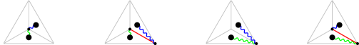
Figure 5: The four possible scenarios for paths between pairs of vertices in $\text{Inter}(R)$. The three colors correspond to the three sub-paths, the red one being the f-edge.

We will first compute a lower bound $\text{Inter}^{-}(R)$ of the interdistance by neglecting the f-edges. This lower bound gives a total distance on pairs of $\text{Inter}(R)$, with $R\in\mathcal{R}_{n}$ order $n^{2}\sqrt{n}$. We can also take an upper bound $\text{Inter}^{+}(R)$ by forcing every path to pass from the center of $R$ and this still gives a contribution of order $n^{2}\sqrt{n}$ with the same factor. Counting the exact number of f-edges allows us to compute the following terms of the interdistance.

4.3.1 Lower bound and upper bound

As for the intradistance we first compute a lower (resp. upper) bound on interdistances at the topmost level $\text{Inter}_{1}(R)$ (i.e. $S_{v},S_{w}\in\mathcal{S}(R)$) and extend it recursively for the whole RANS.

Lemma 4.6.

The generating function for lower bound (resp. upper bound) of the total distance of pairs in $\text{Inter}_{1}(R)$, $\gamma^{-}(z)$ (resp. $\gamma^{+}(z)$), satisfies

$$\gamma^{-}(z)=6z^{2}T(z)T^{\prime}(z)\Delta_{(}2)(z)\qquad\qquad\gamma^{+}(z)=6z^{2}T(z)T^{\prime}(z)\Delta_{(}1)(z).$$

Proof.

At level one, for each sub-RANS, the contribution to the interdistance is the total length of the sub-paths contained in this sub-RANS. Thus for each vertex $v$, situated in a sub-RANS $S_{1}(R)$, we will count its distance to the frontier, multiplied by the number of vertices in $S_{2}(R)$ and $S_{3}(R)$. The lower bound is obtained by adding all these values (parameter $\Delta_{(}2)$), and for the upper bound we consider that the frontier is reduced to only one of its two points (parameter $\Delta_{(}1)$). Thus the expression of the generating function $\gamma^{-}(z)$ (and $\gamma^{+}$ is obtained by replacing $\Delta_{(}2)$ by $\Delta_{(}1)$):

$$\gamma^{-}(z)=3\sum_{R\in\mathcal{R}}\Delta_{(}2)(S_{1}(R))\times(|S_{2}(R)|+|S_{3}(R)|)\,z^{|T|}.$$

∎

Theorem 4.7.

The generating function for the lower bound (resp. upper bound) of interdistances in a RANS is

$$\text{Inter}^{-}(z)=\frac{\gamma^{-}(z)}{1-3zT^{2}(z)}\qquad\qquad\text{Inter}^{+}(z)=\frac{\gamma^{+}(z)}{1-3zT^{2}(z)}$$

and in both cases the total distance between pairs of vertices in $\text{Inter}(R)$, for $R\in\mathcal{R}_{n}$, is asymptotically $Cn^{2}\sqrt{n}$ with $C=\sqrt{3\pi}/11$.

Proof.

The proof is similar to the proof of theorem 4.5. The generating functions $\text{Inter}^{-}(z)$ and $\text{Inter}^{+}(z)$ have both a dominant term in $6\Delta_{(}i)(z)z^{2}T^{\prime 2}(z)/T^{2}(z)$. ∎

4.3.2 Exact computation

To know whether the path between two vertices $(v,w)\in\text{Inter}(R)$ contains a f-edge it helps to know the distances from $v$ and $w$ to each of the two vertices $(f_{1},f_{2})$ of $\text{Frontier}(S_{v},S_{w})$.

We distinguish two cases:

• The first one when either $d(v,f_{1})=d(v,f_{2})$ (we then say that $v\in\mathcal{E}(R)$) or $d(w,f_{1})=d(w,f_{2})$. In this case the path between $v$ and $w$ does not contain a f-edge.

• Otherwise either $v$ and $w$ are both closer to the same vertex of the frontier or each one of them is closer to a different vertex of the frontier. In the first case there is no f-edge on the path between $v$ and $w$ while on the second case there is one.

These two cases being equiprobable, thanks to the symmetry, it is sufficient to calculate the number of pairs $(v,w)\in\text{Inter}(R)$ for which $v,w\notin\mathcal{E}(R)$, and the number of f-edges will be the half of this quantity.

Lemma 4.8.

The generating function for the number of f-edges in the total distance of $\text{Inter}_{1}(R)$ is

$$\phi(z)=\frac{3}{2}\left(z^{3}T(z)T^{\prime 2}(z)-2z^{2}T(z)T^{\prime}(z)E(z)+zT(z)E^{2}(z)\right)$$

where $E(z)=\sum_{R\in\mathcal{R}}|\mathcal{E}(R)|z^{|R|}$.

Proof.

The number of pairs in $\text{Inter}_{1}(R)$ for which $v,w\notin\mathcal{E}(R)$ has generating function

$$\phi(z)=3\sum_{R\in\mathcal{R}}(|S_{1}|-E(S_{1}))(|S_{2}|-E(S_{2}))z^{|R|}.$$

∎

Calculating $E(z)$.

We use a bivariate generating function $T_{e}(z,u)$ for RANS marked with vertices at equal distance from $O_{1}$ and $O_{2}$. This will be defined by a system of thirteen equations in the same spirit as in section 3.1. The analysis of this system is too long to be included in this abstract, but it leads to

$$E(z)=\frac{3zT^{\prime}(z)}{2T^{2}(z)}\,\left(zT^{\prime}(z)-\frac{T(z)(2-4T(z)+3T^{2}(z)-T^{3}(z))}{(2T(z)-3)(3T^{2}(z)-4T(z)+2}\right)^{2}$$

and a singular expansion around $\rho$ which is equivalent to $\frac{5\sqrt{3}}{44}\times(1-z/\rho)^{-1/2}$.

Theorem 4.9.

The generating function for the number of f-edges in a RANS is $F(z)=\phi(z)/(1-3zT^{2}(z))$ and the total number of f-edges in R, for $R\in\mathcal{R}_{n}$, is asymptotically $\frac{9\sqrt{\pi}}{242}n^{2}$.

Proof.

The proof is similar to theorem 4.5. But in this case, each term of $\phi(z)$ gives a part of the dominant contribution. ∎

4.4 Conclusion

Summing the contribution of intradistances and interdistances the enumerating generating function for the total distance between pairs of vertices expresses as:

$$G(z)=\text{Intra}(z)+\text{Inter}^{-}(z)+F(z),$$

which has a closed form expression as a rational function in terms of $z$ and $T(z)$.

We made an exhaustive study of the different parts of $G(z)$. The contribution coming from intradistances happens to be of smaller order ($n^{2}$) than the contribution coming from interdistances ($n^{2}\sqrt{n}$). In the computation of interdistances, we first considered approximations that give a lower and an upper bound with the same dominant term ($\frac{\sqrt{3\pi}}{11}n^{2}\sqrt{n}$) that is a mean distance in $\frac{2\sqrt{3\pi}}{11}\sqrt{n}$. The study of f-edges provides an exact computation of the total distance. With this contribution of f-edges it is possible to express the second term in the asymptotic expression of the total distance. Moreover, relying on full singular expansion of all series under consideration, it is possible to give a full asymptotic expansion of the total distance.

References

- [1] A. Darrasse and M. Soria. Degree distribution of random Apollonian network structures and Boltzmann sampling. Discrete Mathematics and Theoritical Computer Science Proceedings, to appear.
- [2] P. Flajolet and R. Sedgewick. Analytic Combinatorics. Cambridge University Press, 2007.
- [3] M.E.J. Newman, A.L. Barabási and D.J. Watts. The structure and dynamics of networks. Princeton University Press, 2006
- [4] T. Zhou, G. Yan and B.-H. Wang. Maximal planar networks with large clustering coefficient and power-law degree distribution journal. Physical Review E, 71(4):46141, 2005.