X-ray spectral evolution of TeV BL Lac objects:

Abstract

Context. Many of the extragalactic sources detected in $\gamma$ rays at TeV energies are BL Lac objects. In particular, they belong to the subclass of “high frequency peaked BL Lacs” (HBLs), as their spectral energy distributions exhibit a first peak in the X-ray band. At a closer look, their X-ray spectra appear to be generally curved into a log-parabolic shape. In a previous investigation of Mrk 421, two correlations were found between the spectral parameters. One involves the height $S_{p}$ increasing with the position $E_{p}$ of the first peak; this was interpreted as a signature of synchrotron emission from relativistic electrons. The other involves the curvature parameter $b$ decreasing as $E_{p}$ increases; this points toward statistical/stochastic acceleration processes for the emitting electrons.

Aims. We analyse X-ray spectra of several TeV HBLs to pinpoint their behaviours in the $E_{p}-S_{p}$ and $E_{p}-b$ planes and to compare them with Mrk 421.

Methods. We perfom X-ray spectral analyses of a sample of 15 BL Lacs. We report the whole set of observations obtained with the BeppoSAX, XMM-Newton and Swift satellites between 29/06/96 and 07/04/07. We focus on five sources (PKS 0548-322, 1H 1426+418, Mrk 501, 1ES 1959+650, PKS2155-304) whose X-ray observations warrant detailed searching of correlations or trends.

Results. Within our database, we find that four out of five sources, namely PKS 0548-322, 1H 1426+418, Mrk 501 and 1ES 1959+650, follow similar trends as Mrk 421 in the $E_{p}-S_{p}$ plane, while PKS 2155-304 differs. As for the $E_{p}-b$ plane, all TeV HBLs follow a similar behaviour.

Conclusions. The trends exhibited by Mrk 421 appear to be shared by several TeV HBLs, such as to warrant discussing predictions from the X-ray spectral evolution to that of TeV emissions.

1 Introduction

Many multiwavelength observations of BL Lac objects support the view that these are active galactic nuclei (AGNs) with relativistc jets pointing close to the line of sight and emitting continuous, Doppler-boosted spectra with limited photon reprocessing at the source (Blandford & Rees 1978; Urry & Padovani 1995).

The spectral energy distributions (SEDs) of these sources include two main components: a low-energy component with power peaking in the range from the IR to the X-ray band, and a substantial high-energy component often dominated by $\gamma$ rays. It is widely agreed that the low-energy component is produced by synchrotron radiation of ultrarelativistic electrons in the jet. Following the widely entertained synchrotron self-Compton scenario (SSC; e.g. Jones et al., 1974; Ghisellini & Maraschi, 1989) the second component may be interpreted as inverse-Compton scattering of the synchrotron photons by the same electron population.

A classification criterion for BL Lacs was suggested by Padovani & Giommi (1995) on the basis of the location of their first SED peak. This distinguishes the high-frequency peaked BL Lacs (HBLs), for which the peak lies in the UV to the X-ray band, from the low-frequency peaked BL Lacs (LBLs), for which the peak lies in the IR-optical range.

Among the BL Lac objects, several HBLs have been detected at TeV energies, as listed in Table 1. The synchrotron emissions of such HBLs usually peak in the 0.1-10 keV range, and the extensive X-ray observations now available enable precision studies of their spectral shapes. In particular, it is widely known (Landau et al. 1986; Fossati et al. 2000; Massaro et al. 2004) that the spectra and therefore the SEDs of BL Lacs often appear to be intrinsically curved.

A recent analysis of Mrk 421 observations performed with BeppoSAX, XMM-Newton  and ASCA (Tramacere et al. 2007a) has shown two correlations between spectral parameters: the SED peak energy $E_{p}$ correlates with the peak flux $S_{p}$ but anticorrelates with the curvature parameter $b$ (as detailed in Sect. 3). These correlations are relevant as signatures of synchrotron emission and of statistical/stochastic acceleration mechanisms for the emitting electrons, respectively.

In the present paper, we use a wide set of archival data to investigate the X-ray spectral evolution of other TeV HBLs including all BeppoSAX, XMM-Newton and Swift published and unpublished archival observations performed between June 1996 and April 2007. Here, we use the spectra of Mrk 421 (discussed in Tramacere et al., 2007a) as a comparison term for the behaviour of other HBLs. We do not consider in detail BL Lacertae, recently detected at TeV energies (Albert et al. 2006b), as it belongs to the LBL class; its spectral behaviour will be discussed in a separate paper (Fuhrmann et al., 2007)

Table 1: A list of the BL Lacs currently detected at TeV energies. Col. (1) reports source names, Cols.(2,3) the right ascension and declination, respectively, Col. (4) gives the redshift (from NED), Cols. (5,6) the galactic column density along the line of sight: (^∗ Lockman & Savage 1995; ^∗∗ Kalberla et al. 2005), Cols. (7,8,9) report the observing satellite and number of observations, and the final Col. (10) reports the TeV detections. In this paper, we will not pursue Mrk 421 and BL Lac, as anticipated in Sect. 1.

Name	$RA$	$DEC$	$z$	$N_{H,Gal}^{(*)}$	$N_{H,Gal}^{(**)}$		Satellite		TeV detection
				$[10^{20}cm^{-2}]$	$[10^{20}cm^{-2}]$
1ES 0229+200	02 32 48.6	+20 17 17	0.140	9.21	7.69	BeppoSAX (1)			$HESS^{(1)}$
1ES 0347-121	03 49 23.2	-11 59 27	0.185	3.64	3.00	BeppoSAX (1)	xmm (1)	swf (1)	$HESS^{(1)}$
PKS 0548-322	05 50 40.6	-32 16 16	0.069	2.21	2.69	BeppoSAX (3)	xmm (2)	swf (16)	$HESS^{(1)}$
1ES 1011+496	10 15 04.1	+49 26 01	0.210	0.79	0.82			swf (3)	$MAGIC^{(2)}$
1H 1100-230	11 03 37.6	-23 29 30	0.186	5.76	5.60	BeppoSAX (2)	xmm (2)	swf	$HESS^{(3)}$
Mrk 421	11 04 27.3	+38 12 32	0.030	1.61	1.53	BeppoSAX	xmm	swf	$Whipple^{(4)}$
Mrk 180	11 36 26.4	+70 09 27	0.045	1.41	1.20	BeppoSAX (1)	xmm (1)	swf (2)	$MAGIC^{(5)}$
1ES 1218+304	12 21 21.9	+30 10 37	0.182	1.73	1.81	BeppoSAX (1)	xmm (1)	swf (7)	$MAGIC^{(6)}$
1H 1426+428	14 28 32.6	+42 40 21	0.129	1.38	1.10	BeppoSAX (1)	xmm (7)	swf (7)	$CAT^{(7)}$
1ES 1553+113	15 55 43.0	+11 11 24	—-	3.67	3.72	BeppoSAX (1)	xmm (1)	swf (3)	$HESS^{(8)}$
Mrk 501	16 53 52.2	+39 45 37	0.033	1.71	1.42	BeppoSAX (11)	xmm (2)	swf (10)	$Whipple^{(9)}$
1ES 1959+650	19 59 59.8	+65 08 55	0.047	10.0	10.1	BeppoSAX (3)	xmm (3)	swf  (10)	$Whipple^{(10)}$
PKS 2005-489	20 09 25.4	-48 49 54	0.071	5.08	3.80	BeppoSAX (2)	xmm (3)	swf (3)	$HESS^{(11)}$
PKS 2155-304	21 58 52.0	-30 13 32	0.116	1.69	1.42	BeppoSAX (3)	xmm (15)	swf (22)	$HESS^{(12)}$
BL Lac	22 02 43.3	+42 16 40	0.069	21.3	17.1	BeppoSAX		swf	$MAGIC^{(2)}$
1ES 2344+514	23 47 04.8	+51 42 18	0.044	16.3	14.2	BeppoSAX (7)		swf (3)	$Whipple^{(13)}$
1H 2356-309	23 59 07.9	-30 37 41	0.165	1.33	1.36	BeppoSAX (1)	xmm (2)		$HESS^{(3)}$

(1) http://www.mpi-hd.mpg.de/hfm/HESS/HESS.html; (2) http://wwwmagic.mppmu.mpg.de/index.en.html; (3) Aharonian et al. 2006a; (4) Punch et al. 1992; (5) Albert et al. 2006a; (6) Albert et al. 2006b; (7) Djannati-Ataj et al. 2002; (8) Aharonian et al. 2006b; (9) Quinn et al. 1996; (10) Nishiyama et al. 1999; (11) Aharonian et al. 2005a; (12) Chadwick et al. 1999; (13) Catanese et al. 1998.

2 Observations and data reduction

2.1 BeppoSAX

Our data set includes the BeppoSAX observations of our sample sources performed with the narrow field instruments (NFIs): LECS ($0.1-10$ keV; Parmar et al. 1997), MECS ($1.3-10$ keV; Boella et al. 1997) and PDS ($13-300$ keV; Frontera et al. 1997). Events for spectral analysis were extracted following standard procedures. In particular, LECS and MECS events were selected in circular regions centred at the source position, with radii of 4’ and 8’ depending upon the count rate, as indicated by Fiore et al. (1999). The response matrices and the ancillary response files used in our analysis have been taken from the BeppoSAX SDC ftp server (September 1997 release), and background spectra were taken from the blank field archive. Standard procedures and selection criteria were applied to the data to avoid the South Atlantic geomagnetic anomaly, and the solar, bright Earth and particle contaminations using the SAXDAS (v. 2.0.0) package.

2.2 XMM-Newton

Our sources were observed with XMM-Newton  between May 2000 and May 2006 by means of all EPIC CCD cameras: the EPIC-PN (Struder et al. 2001), and EPIC-MOS (Turner et al. 2001), operating in different modes and with different filters, as described in Appendix A. Only EPIC-MOS data were reported in this work.

These data are reduced with the same procedure described in Tramacere et al. (2007a). Extractions of all light curves, source and background spectra are done using the XMM-Newton  Science Analysis System (SAS) v6.5.0. The calibration index file (CIF) and the summary file of the observation data file (ODF) were generated using updated calibration files (CCF) following the “User’s Guide to the XMM-Newton  Science Analysis System” (issue 3.1, Loiseau et al. 2004) and “The XMM-Newton  ABC Guide” (vers. 2.01, Snowden et al. 2004). Event files were produced by the XMM-Newton  EMCHAIN pipeline.

Light curves for every dataset are extracted, and all high-background time intervals are filtered out to exclude those contaminated by solar flare signals. Then, by visual inspection, we select good time intervals far from solar flare peaks and with no count rate variations on time scales shorter than 500 seconds.

Photons are extracted from an annular region using different apertures to minimise pile-up, which affects MOS data. The typical value of the external radius for the annular region is $40$ ^′′. To filter out pixels affected by significant pile-up, the internal region was selected by using the EPATPLOT task in XMM-Newton (SAS) for each observation, following the same procedure used in Tramacere et al. (2007a) (for details, see also Loiseau et al. 2004; Snowden et al. 2004).

In FULL WINDOW images, the background spectrum is extracted from a circular region with size comparable to the source region, in a position where sources are not present (typically off axis). For other observations, in PARTIAL WINDOW images, no regions are found sufficiently far from the source for background extraction; in these cases we use background from blank-field event files (www.sr.bham.ac.uk). In all cases, we estimate that the average X-ray background flux was always at $\sim$ 1% levels of the source flux, resulting in a negligible contamination of the spectral parameter determination. A restricted energy range (0.5–10 keV) is used to avoid possible residual calibration uncertainties. To ensure the validity of $\chi^{2}$ statistics, data are grouped by combining instrumental channels so that each new bin comprises 40 counts or more, well above the limit for the $\chi^{2}$ test applicabilty (Kendall & Stuart, 1979).

2.3 Swift

The XRT data analysis is performed with the XRTDAS software (v. 2.1), developed at the ASI Science Data Center (ASDC) and included in the HEAsoft package (v. 6.0.2). Event files were calibrated and cleaned with standard filtering criteria using the xrtpipeline task combined with the latest calibration files available in the Swift CALDB distributed by HEASARC. Events in the energy range 0.3–10 keV with grades 0–12 (photon counting mode, PC) and 0–2 (windowed timing mode, WT) are used in the analyses (see Hill et al. 2004 for a description of readout modes, and Burrows et al. 2005 for a definition of XRT event grades). To avoid artificially high $\chi^{2}$ values and possible biases in spectral parameter estimations, we follow the advice of the XRT calibration experts, and exclude from our analysis the energy channels between 0.4 keV and 0.6 keV (Campana & Cusumano 2006, private communication).

For the WT mode data, events are selected for temporal and spectral analysis using a 40 pixel wide (1 pixel $=2.36$ arcs) rectangular region centred on the source, and aligned along the WT one dimensional stream in sky coordinates. Background events are extracted from a nearby source-free rectangular region of 40 pixels width and 20 pixels height.

For PC mode data, when the source count rate was above $\sim$ 0.5 counts s^-1 the data were significantly affected by pile-up in the inner part of the point spread function (PSF). To remove the pile-up contamination, we extract only events contained in an annular region centred on the source. The inner radius of the region was determined comparing the observed PSF profiles with the analytical model derived by Moretti et al. (2005), and tipically has a 4 or 5 pixels size, while the outer radius is 20 pixels for each observations. For Swift observations in which the source count rate was below the pile-up limit, events are instead extracted using a 20 pixel radius circle. The background for PC mode is estimated from a nearby source-free circular region of 20 pixel radius.

Ancillary response files are generated with the xrtmkarf task applying corrections for the PSF losses and CCD defects. The latest response matrices (v. 009) available in the Swift CALDB are used, and source spectra are binned to ensure a minimum of 30 counts per bin in order to utilize the $\chi^{2}$ minimisation fitting technique and ensure the validity of $\chi^{2}$ statistics.

3 Spectral analysis

We perform our spectral analysis with the xspec software package, version 11.3.2 (Arnaud, 1996). We describe the X-ray continuum with different spectral models: an absorbed power-law with column density either free, or fixed at the Galactic value; a power-law with an exponential cutoff; a log-parabolic model (Landau et al. 1986; Massaro et al. 2004). The latter two models are absorbed by a Galactic column density (see Table 1).

The log-parabolic model is tested under the form

$$F(E)=K\leavevmode\nobreak\ E^{-a-b\leavevmode\nobreak\ log(E)}\leavevmode\nobreak\ \leavevmode\nobreak\ \leavevmode\nobreak\ [photons\leavevmode\nobreak\ cm^{-2}\leavevmode\nobreak\ s^{-1}\leavevmode\nobreak\ keV^{-1}],$$ (1)

or the alternative SED representation

$$S(E)=S_{p}\leavevmode\nobreak\ 10^{-b\leavevmode\nobreak\ log^{2}(E/E_{p})}\leavevmode\nobreak\$$ (2)

with $S_{p}=E_{p}^{2}\,F(E_{p})$. After Eq. (2), the values of the parameters $E_{p}$ (the location of the SED energy peak), $S_{p}$ (the peak height), and $b$ (the curvature parameter) can be estimated independently in the fitting procedure (Tramacere et al. 2007a). In all models with fixed Galactic column density, we use $N_{H}$ values from the LAB survey (Kalberla et al., 2005) or from (Lockman & Savage 1995), as reported in Table 1. We find consistent spectral parameters (within a 1$\sigma$ interval) from these two column densities. Tables A.1, A.2 and A.3 report the results from the spectral analyses performed with the standard $N_{H}$ values from Lockman & Savage (1995).

Typically, the X-ray spectra of HBLs appear to be featurless and curved (Giommi et al. 2005; Perri et al. 2007) over a broad energy range. Absence of spectral features related to any absorbing material was also recently confirmed by Blustin et al. (2004), who performed a detailed analysis of XMM-Newton RGS spectra of four sources in our sample, namely 1H 1219+301, 1H 1426+428, Mrk 501 and PKS 0548-322.

With an absorbed power-law model we usually obtain unacceptable values of $\chi^{2}_{r}$; even when we leave the low energy absorption as a free parameter, these models are not adequate to describe the high energy end of the X-ray spectra. Adding to a power-law model, a high energy exponential cutoff $E_{c}$ corrects the residuals at high energies, however, values of $E_{c}$ beyond the instrumental energy range are often obtained. In a few cases where we find an exponential cutoff within the observed energy range, the $\chi^{2}_{r}$ values are significantly higher than those found with the log-parabolic model. In some cases, poor statistics (due to short observational exposures) or restricted instrumental energy range (XMM-Newton and Swift relative to BeppoSAX), combined with the location of the SED peak outside the observational energy range, make it difficult to evaluate a possible spectral curvature; here, the single power-law model constitutes an acceptable description of the X-ray spectra.

Analyses of long exposure pointings are performed using time-resolved spectra, as described in Tramacere et al. (2007a), to avoid averaging significant spectral variations while still conserving a sufficient number of counts per observation as to evaluate the spectral curvature. Results of our spectral analyses are reported in Appendix A; the statistical uncertaintes quoted refer to the 68% confidence level (one Gaussian standard deviation). Observations with less than 30 energy bins after the rebinning procedure or with less than 800 seconds of exposure were not considered for these analyses.

In conclusion, in agreement with other previous X-ray analyses (Massaro et al. 2004; Massaro et al. 2006; Tramacere et al. 2007a; Tramacere et al. 2007b; Perlman et al. 2005), we find that for about 70% of all observations the best description for synchrotron spectra of HBLs close to their peak energy is provided by a log-parabolic model. The percentage increases to 99% for observations with exposures longer than 2000 seconds.

4 Results

Two significant correlations between spectral parameters of the log-parabolic model were found by Tramacere et al. (2007a) from studying the X-ray synchrotron emission of Mrk 421. Specifically, $S_{p}$ increases with $E_{p}$ while the curvature $b$ decreases. Here, we look for any similar correlations or trends in other TeV HBLs. For effective comparisons it is necessary to make cosmological corrections, even though the redshift range of these sources is rather narrow. In the log-log representation, the redshift rescaling corresponds to a translation of the spectral energy distribution to higher energies with a increased height. The curvature parameter $b$, as defined by Eqs.(1) and (2), is not afffected while the other parameters, $E_{p}$ and $S_{p}$, are.

In particular, the rest frame energy peak $E_{p}^{*}$ is given by

$$E_{p}^{*}=(1+z)\leavevmode\nobreak\ E_{p}.$$ (3)

In addition, noting that the value of $S_{p}$ is proportional to the bolometric emitted flux, we compare the rest frame powers of BL Lacs in terms of the isotropic luminosity peak energy $L_{p}^{*}$:

$$L_{p}^{*}\simeq 4\pi D_{L}^{2}S_{p}.$$ (4)

Here, the luminosity distance $D_{L}$ of our sources is given by (Peebles, 1993):

$$D_{L}=\frac{c}{H_{0}}(1+z)\int_{0}^{z}\frac{dz}{\sqrt{\Omega_{M}(1+z)^{3}+\Omega_{\Lambda}}},$$ (5)

using a flat cosmology with $H_{0}=72$ km/(s Mpc), $\Omega_{M}=0.27$ and $\Omega_{\Lambda}=0.73$ (see Spergel et al., 2007).

To search for trends, one needs at least 10 observations with $E_{p}$, $S_{p}$, $b$ well estimated, a requirement satisfied by only 5 of our sources, namely PKS 0548-322, 1H 1426+418, MRK 501, 1ES 1959+650 and PKS 2155-304. For these sources we perform spectral analyses to evaluate independently $E_{p}$, $S_{p}$, $b$, to which we apply the redshift corrections discussed above.

We investigate the presence of trends by evaluating the linear correlation coefficient $r_{log}$ between the logarithms of spectral parameters. For Mrk 421, the results are $r_{log}=0.67$ and $r_{log}=-0.67$ for the $E_{p}^{*}-L_{p}^{*}$ and $E_{p}^{*}-b$ relations, respectively. In Figs. 1, 2, 4, 6 and 8, we plot the values of the spectral parameters, with their uncertanties, for each of the five sources and include those of Mrk 421 for comparison.

Figure 1 shows the results for PKS 0548-322; it is worth noting that in this source both $E_{p}^{*}$ and $L_{p}^{*}$ vary in a narrower range compared to Mrk 421. PKS 0548-322 follows the same trend of Mrk 421 on both the $E_{p}^{*}-L_{p}^{*}$ and $E_{p}^{*}-b$ planes, with correlation coefficients $r_{log}=0.61$ and $r_{log}=-0.60$, respectively.

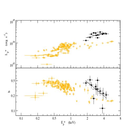
Figure 1: $E_{p}^{*}-L_{p}^{*}$ and $E_{p}^{*}-b$ plots for PKS 0548-322 (black filled squares) compared with those of Mrk 421 (orange circles). Black lines indicate the regressions underlying the $r_{log}$ correlation coefficient.

The source 1H 1426+428 has a similar behaviour to Mrk 421 in the $E_{p}^{*}-L_{p}^{*}$ and $E_{p}^{*}-b$ plots (see Fig. 2), even though it is an order of magnitude brighter than the latter. In this figure, we also show the XMM-Newton observation performed on 16 June 2001 (circled in the figure), in which the log-parabolic bestfit indicates a value of $E_{p}^{*}$ beyond the instrumental energy range; this circumstance makes the formal uncertainty unreliable, and motivates us to exclude this pointing from our statistical analysis. The observation of XMM-Newton  on 16 June 2001 appears to confirm the statistical trend in the $E_{p}^{*}-b$ plane, but in the $E_{p}^{*}-L_{p}^{*}$ plane it lies in a different position relative to other pointings. As shown in Fig. 3, during this particular pointing, 1H 1426+428 shifted its SED peak energy without large variation of $L_{p}^{*}$, at variance with the following ones by XMM-Newton. We find correlation coefficients $r_{log}=0.72$ for the $E_{p}^{*}-L_{p}^{*}$ relation, and $r_{log}=-0.47$ for the $E_{p}^{*}-b$ one; these confirm the similarity to Mrk 421 and to PKS 0548-322. Note that 1H 1426+428 also covers similar regions on the $E_{p}^{*}-L_{p}^{*}$ and $E_{p}^{*}-b$ to Mrk 421.

Figure 2: $E_{p}^{*}-L_{p}^{*}$ and $E_{p}^{*}-b$ plots for 1H 1426+428 (black filled squares) compared with those of Mrk 421 (orange circles). Black lines indicate the regressions underlying the $r_{log}$ correlation coefficient. Circled values refers to the peculiar observation performed on the 16 June 2001 by XMM-Newton  (see Sect. 4 for details).

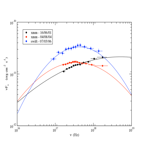
Figure 3: The SEDs for three observations of 1H 1426+428 performed by XMM-Newton and Swift.

For Mrk 501 the $E_{p}^{*}-L_{p}^{*}$ and $E_{p}^{*}-b$ plots are shown in Fig. 4. Here the range of $E_{p}^{*}$ is wider and the luminosities are higher compared to Mrk 421. Figure 5 shows in detail the strong variability of this source. The source has similar trends to Mrk 421, with higher correlation coefficients for the $E_{p}^{*}-L_{p}^{*}$ and $E_{p}^{*}-b$ relations, namely, $r_{log}=0.89$ and $r_{log}=-0.79$, respectively. Figure 5 shows the SEDs relative to three observations performed with all three satellites to show in detail the variations of $E_{p}$, $s_{p}$, and curvature $b$.

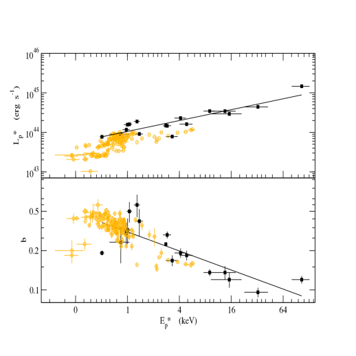
Figure 4: $E_{p}^{*}-L_{p}^{*}$ and $E_{p}^{*}-b$ plots for Mrk 501 (black filled squares) compared with those of Mrk 421 (orange circles). Black lines indicate the regressions underlying the $r_{log}$ correlation coefficient.

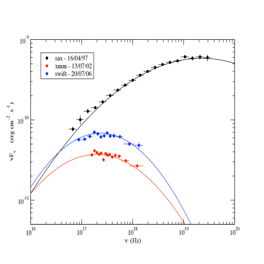
Figure 5: The SEDs for three observations of Mrk 501 performed by BeppoSAX, XMM-Newton and Swift.

The observations of 1ES 1959+650 cover a narrower subregion of both the $E_{p}^{*}-L_{p}^{*}$ and the $E_{p}^{*}-b$ plane relative to Mrk 421, as shown by Fig 6. These observations were mostly performed within ten days during 2006. The observation performed on 29 May 2006 (circled) is peculiar as it yields a very high curvature value. This pointing took place at the end of a set of 6 observations, in which the flux was decreasing; this may represent a phase dominated by cooling, when the estimated value of the curvature could well be affected by an exponential cutoff close to the observed energy range.

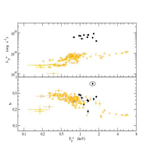
Figure 6: $E_{p}^{*}-L_{p}^{*}$ and $E_{p}^{*}-b$ plots for 1ES 1959+650 (black filled squares) compared with those of Mrk 421 (orange circles). Circled values refers to the peculiar observation performed on the 29 May 2006 by Swift  (see Sect. 4 for details).

The source PKS 2155-304 is the truly variant member of our set in a number of respects. In fact, the spectral analysis yields a log-parabolic index $a>2$, and relatedly, $E_{p}$ is less than 1 keV. It was difficult to evaluate the SED peak location with BeppoSAX, XMM-Newton and Swift  because it often falls below the observational X-ray range, as shown in Fig. 7. Such spectra indicate that the X rays constitute the upper end of a synchrotron emission. On the other hand, we never observed a high energy exponential cutoff in our analysis, which confirmes our modelling in terms of a spectral curvature $b$. The source PKS 2155-304 covers a region in the $E_{p}^{*}-b$ plane overlapping that of Mrk 421 in Fig. 8. On the other hand, the same figure shows that the source does not appear to follow a similar trend in the $E_{p}^{*}-L_{p}^{*}$ plane. A possible explanation for this is that our X-ray observations may be biased in that we observe the source only with $E_{p}$ values in the X-rays band, corresponding to higher states relative to its average (Tramacere et al., 2007b).

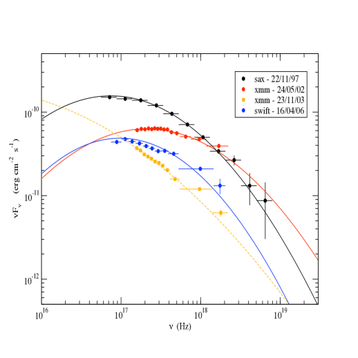
Figure 7: The SEDs for four observations of PKS 2155-304 performed by BeppoSAX, XMM-Newton and Swift.

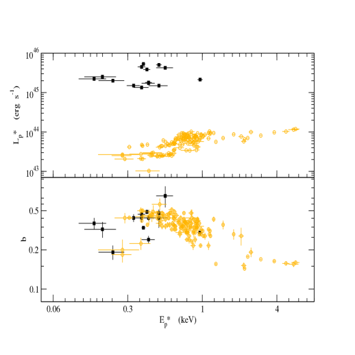
Figure 8: $E_{p}^{*}-L_{p}^{*}$ and $E_{p}^{*}-b$ plots for PKS 2155-304 (black filled squares) compared with those of Mrk 421 (orange circles).

5 Discussion

Correlations between $L_{p}^{*}$ and $E_{p}^{*}$ provide interesting information concerning the driver of the source spectral evolution. For example, using a wide dataset of X-ray observations of Mrk 421 we have investigated the effects of varing physical parameters in the synchrotron emission, where the dependence of $L_{p}^{*}$ on $E_{p}^{*}$ may be represented in the form of a power-law, that is, $L_{p}^{*}\propto E_{p}^{*\leavevmode\nobreak\ \alpha}$ (Tramacere et al., 2007a, and references therein).

In fact, the synchrotron peak is expected to scale as $L_{p}^{*}\propto N\leavevmode\nobreak\ \gamma^{2}\leavevmode\nobreak\ B^{2}\leavevmode\nobreak\ \delta^{4}$ while the peak energy scales as $E_{p}^{*}\propto\gamma^{2}B\leavevmode\nobreak\ \delta$, in terms of the number $N$ of emitting particles, the magnetic field $B$, of the typical electron energy $\gamma mc^{2}$, and of the beaming factor $\delta$. Thus, $\alpha=1$ applies when the spectral changes are dominated by variations of the electron average energy, $\alpha=2$ applies for changes of the magnetic field, $\alpha=4$ if changes in the beaming factor dominate and formally, $\alpha=\infty$ (i.e., a vertical line in the $E_{p}^{*}-L_{p}^{*}$ plane) applies for changes only in the number of emitting particles.

Here, we have presented accurate analyses of the X-ray spectra of several TeV HBLs observed over a period 11 years. We confirm that these spectra are best described with a log-parabolic model, even though in some cases an acceptable fit is also provided by a power-law spectral model absorbed by a Galactic column density.

From our analyses we have derived values of spectral parameters, $E_{p}$, $S_{p}$ and curvature $b$, independently. With the cosmological transformations given by Eqs. (3) and (5), we searched for possible correlations, or at least trends, among the spectral parameters. Five sources (PKS 0548-322, 1H 1426+428, Mrk 501, 1ES 1959+650, PKS2155-304) have enough data to warrant investigating in some detail the $E_{p}^{*}-L_{p}^{*}$ and $E_{p}^{*}-b$ relations and comparing them with those found for Mrk 421.

On the other hand, the number of observations for each source in our sample does not allow statistical analyses as detailed as in the case of Mrk 421 (Tramacere et al. 2007a). Therefore for these sources it is not yet possible to determine the value of the synchrotron exponent $\alpha$. Accordingly, we have evaluated only the logarithmic correlation coefficients $r_{log}$ between $E_{p}^{*}-L_{p}^{*}$ and $E_{p}^{*}-b$ for each source.

Comparing these values with those evaluated for Mrk 421 we have found that at least three sources (namely PKS 0548-322, 1H 1426+428 and Mrk 501) follow the same trends as Mrk 421 in the $E_{p}^{*}-L_{p}^{*}$ plane. In the case of 1ES 1959+650, our observed spectral parameters cover a smaller region compared to Mrk 421; nevertheless, the trend so outlined is consistent with that of the latter. Finally, we have found that PKS 2155-304 has again a similar behaviour in the $E_{p}^{*}-b$ plane but definitely a different one in the $E_{p}^{*}-L_{p}^{*}$ plane.

An overall comparison of these similarities is given in Fig. 9 (upper panel). This portrays the $E_{p}^{*}-b$ plane for these five sources plus Mrk 421, to show that the curvature ranges from about 0.12 to about 0.55 (with the exception of only one pointing of 1ES 1959+650, as discussed above); the correlation coefficient for the sample constituted by these sources is $r_{log}=-0.66$. Examination of Tables A1, A2 and A3 indicates that the remaining sources in our sample are consistent with the trend estabilished for Mrk 421 and confirmed by the five HBLs discussed above (see also Fig. 9 lower panel).

Next, we point out two cautionary remarks on biases that may arise when comparing analyses of different sources. First, we note the role of the beaming factor. Although Tramacere et al. (2007a) show that for Mrk 421 the beaming factor is unlikely to be the main driver of the $E_{p}^{*}-L_{p}^{*}$ relation, it may play a subtler role when comparing several sources. In fact, both $E_{p}^{*}$ and $L_{p}^{*}$ depend on $\delta$; this implies that even though for a single source $\delta$ does not have a large variation, its value may vary significantly from source to source, affecting the $E_{p}^{*}-L_{p}^{*}$ plot. The same holds for the magnetic field intensity. A second effect may be given by a poor temporal sampling. Sources observed sporadically, with observations covering short temporal intervals, may be representative only of flaring or of low emission states, thus producing an uneven coverage of the parameter space.

Finally, we outline a link between the synchrotron peak and the TeV emissions. In fact, within a single zone SSC scenario, we expect that synchrotron signatures derived from X-rays observations have counterparts in the TeV energy range, where the inverse Compton peak lies. In closer detail, we expect the inverse Compton peak height $C_{p}^{*}$ and its location $\epsilon_{p}^{*}$ in energy to be given by

$$C_{p}^{*}\propto N^{2}R^{-2}\gamma^{4}B^{2}\delta^{4}\\ \epsilon_{p}^{*}\propto\gamma^{4}B\delta\leavevmode\nobreak\ \leavevmode\nobreak\ \leavevmode\nobreak\ \leavevmode\nobreak\ \leavevmode\nobreak\ (Thomson\leavevmode\nobreak\ regime)$$ (6)

$$C_{p}^{*}\propto NR^{-2}B\delta^{4}\\ \epsilon_{p}^{*}\propto\delta\gamma\leavevmode\nobreak\ \leavevmode\nobreak\ \leavevmode\nobreak\ \leavevmode\nobreak\ \leavevmode\nobreak\ (Klein-Nishina\leavevmode\nobreak\ regime),$$ (7)

where $R$ is the size of the emitting region. It transpires that a definite link exists between the correlations for the variations of the synchrotron peak and variability of the inverse Compton peak, an issue that we plan to discuss in full in a forthcoming paper.

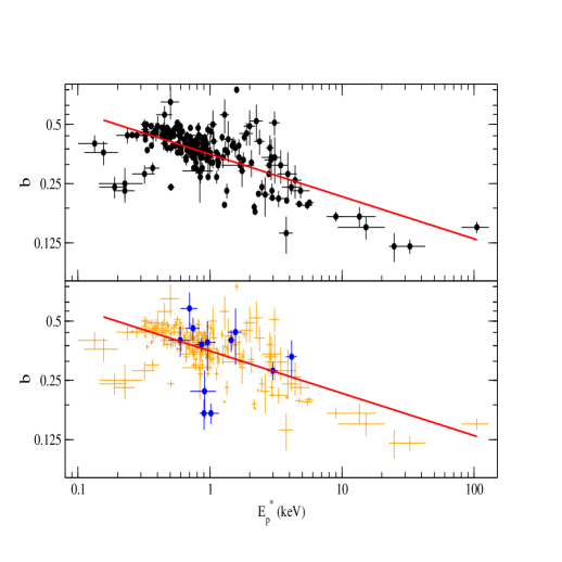
Figure 9: Upper panel: the $E_{p}^{*}-b$ plot for Mrk 421 and for the five sources analysed in detail in Sect. 5. Lower panel: blue points represents the other TeV HBLs with insufficient data to perform a detailed analysis. The above sources are replotted with orange crosses.

6 Conclusions

In the present paper, we have conducted an X-ray study of 15 HBL sources, also detected at TeV energies, to investigate their synchrotron emission. Our main results are summarised as follows.

We confirm that the log-parabolic model provides the best description for the X-ray spectra of HBLs, when the statistics are sufficient to warrant evaluating a spectral curvature. We show that several HBLs detected at TeV energies share the same trends found for Mrk 421 in the $E_{p}^{*}-L_{p}^{*}$ and $E_{p}^{*}-b$ planes. In particular, for the $E_{p}^{*}-b$ relation, all HBLs in our sample cover the same region of these parameter’s plane, with the curvature $b$ always decreasing with increasing $E^{*}_{p}$. Finally, we outline a link of the TeV emission with the synchrotron peak in a single zone SSC scenario.

Appendix A Spectral analysis of the HBL sample

Tables A.1, A.2 and A.3 report the log of our observations and the values of the spectral parameters we have derived for TeV HBLs in our sample.

In Table A.1, $LECS$, $MECS$ and $PDS$ columns indicate the exposure time in seconds. The BeppoSAX spectral analysis of 1ES 0347-121, 1ES 1011+492, PKS 2344-514 is reported in Giommi et al. (2005, also available at http://www.asdc.asi.it/sedentary/).

In Table A.2, $Frame$ indicates the EPIC camera used (M1$=$MOS1 and M2$=$MOS2), the modes (PW$=$partial window and FW$=$full window) and the filter (Th$=$thin, Md$=$medium, Tk$=$thick) used for each pointing (see Sect. 2.2 for details), and the exposure is reported in seconds in the column $Exps$. In Table A.2 capital letters near the observation date indicate a different pointing in the same observation, while lower case letters refer to time resolved spectra (see also Tramacere et al. 2007a). The capital letter $F$ in the last column XMM-Newton table (A.2) indicates that the observation is too contaminated by solar flares to be used in our spectral analysis.

In Swift Table A.3 the column $Frame$ reports on the observation modality (PC for photon counting and WT for windowed timed, see also Sect. 2.3 for details), and $Exps$ means the exposure time in seconds.

All other columns in each table refer to the log-parabolic model bestfit. When the value estimated for a spectral parameter is consistent with zero in a $3\sigma$ interval, the values reported in each table refer to the power-law model bestfit (see Sects. 3 and 4). In these cases, the curvature parameter $b$, the SED peak energy $E_{p}$ and the corresponding SED peak height $S_{p}$ cannot be reliably evaluated, and are marked with a dashed line. Values of $E_{p}$ are reported in $keV$, the normalisation $K$ in units of $10^{-4}photons\leavevmode\nobreak\ cm^{-2}\leavevmode\nobreak\ s^{-1}\leavevmode\nobreak\ keV^{-1}$ and $S_{p}$ in units of $10^{-13}erg\leavevmode\nobreak\ cm^{-2}\leavevmode\nobreak\ s^{-1}$ with $F_{X}$ denoting the $2-10$ $keV$ flux measured in units of $10^{-11}erg\leavevmode\nobreak\ cm^{-2}\leavevmode\nobreak\ s^{-1}$. For spectra with less than 30 bins we report only the estimate of the X-ray flux $F_{X}$ with a power-law model absorbed by a galactic column density (see Sect. 3 for details).

Table 2: BeppoSAX spectral analysis results.

Obs ID	$Date$	$LECS$	$MECS$	$PDS$	$a$	$b$	$E_{p}$	$K$	$S_{p}$	$F_{X}$	$\chi^{2}_{r}$
1ES 0229+200
51472001	16/07/01	17236	68200	33113	1.60(0.10)	0.31(0.08)		43(4)		1.24	0.96(101)
PKS 0548-322
50493003	20/02/99	5642	12439	9355	1.53(0.07)	0.51(0.07)	2.88(0.27)	75(5)	153.6(3.2)	2.02	1.21(67)
50493004	26/02/99	—-	2025	1003	2.40(0.14)	——–	——–	12(2)	———-	1.76	1.31(29)
504930042	07/04/99	5251	18943	10164	1.77(0.07)	0.45(0.06)	1.77(0.21)	67(5)	115.2(4.8)	1.36	0.98(67)
1ES 1101-232
50064017	04/01/97	6146	13868	10676	1.64(0.08)	0.33(0.07)	3.50(0.33)	120(7)	241.6(3.2)	3.71	1.08(184)
50726001	19/06/98	—-	24817	10792	1.97(0.22)	——–	——–	145(4)	———-	2.55	1.31(80)
Mrk 180
50064010	10/12/96	5165	18205	7330	2.24(0.08)	0.28(0.08)	0.37(0.16)	36(4)	65.6(14.4)	0.51	0.91(56)
1ES 1218+304
50863005	12/07/99	10609	42693	20670	2.11(0.03)	0.38(0.03)	0.73(0.08)	98(3)	158.4(6.4)	1.48	0.75(101)
1H 1426+428
50493006	08/02/99	—-	40657	20432	2.22(0.11)	——–	——–	103(16)	———-	2.04	0.95(80)
1ES 1553+113
50064005	05/02/98	4421	10592	4671	2.17(0.07)	0.63(0.08)	0.73(0.11)	115(8)	190.4(1.6)	1.29	1.22(67)
Mrk 501
50377001∗	07/04/97	12387	20571	8936	1.68(0.01)	0.17(0.01)	8.7(1.3)	624(8)	1410(50)	21.5	–
50377002∗	11/04/97	12559	20391	8719	1.64(0.01)	0.12(0.01)	31.6(9.6)	609(7)	1800(100)	23.9	–
50377003∗	16/04/97	9612	17125	7347	1.41(0.01)	0.15(0.01)	101.6(23.7)	960(10)	6000(500)	52.4	–
50529001∗	28/04/98	13552	21892	9873	1.65(0.02)	0.15(0.02)	14.7(5.7)	474(8)	1200(100)	17.6	–
50529002∗	29/04/98	14661	21417	9662	1.62(0.02)	0.17(0.02)	13.1(4.3)	543(8)	1400(100)	20.8	–
50529003∗	01/05/98	13164	19033	8447	1.71(0.02)	0.24(0.02)	4.0(0.6)	477(8)	940(30)	14.7	–
50666001∗	20/06/98	98363	25861	11566	1.79(0.02)	0.21(0.02)	3.2(0.5)	175(4)	320(10)	4.95	–
50666002∗	29/06/98	12682	47528	7470	1.69(0.02)	0.23(0.02)	4.7(0.8)	323(6)	660(30)	10.3	–
50666003∗	16/07/98	11228	15924	6919	1.70(0.02)	0.33(0.02)	2.8(0.3)	320(7)	600(20)	9.0	–
50666004∗	25/07/98	25067	30937	14505	1.76(0.01)	0.28(0.01)	2.7(0.1)	337(5)	610(10)	9.3	–
50944001∗	10/06/99	10405	17510	—-	2.15(0.01)	0.24(0.01)	0.49(0.03)	186(2)	315(4)	3.02	–
1ES 1959+650
50064002	04/05/97	2252	12391	5393	2.02(0.18)	——–	——–	192(14)	———-	1.77	0.90(56)
51386001	23/09/01										P.
513860011	28/09/01	25255	48037	22416	1.79(0.03)	0.43(0.02)	1.74(0.08)	464(9)	785.6(6.4)	10.35	2.00(125)
PKS 2005-489
50046001	29/09/96	—-	9911	7674	2.02(0.19)	——–	——–	268(12)	—–	5.94	1.36(79)
50503002	01/11/98	20067	52467	23437	2.01(0.02)	0.17(0.02)	0.95(0.14)	821(12)	1313.6(19.2)	15.45	1.03(120)
PKS 2155-304
50016001	20/11/96	35644	10686	—-	2.43(0.01)	0.24(0.01)	0.13(0.01)	504(4)	1240.0(28.8)	5.37	1.22(127)
50160008	22/11/97	22086	59497	28007	2.38(0.01)	0.37(0.01)	0.30(0.01)	780(8)	1569.0(27.2)	8.23	1.75(125)
50880001	04/11/99	45208	10392	49144	2.66(0.01)	0.20(0.01)	——–	292(4)	1635.2(118.4)	2.48	1.39(125)
PKS 2354-315
50493007	21/06/98	15055	40950	18034	1.77(0.03)	0.28(0.03)	2.57(0.22)	90(3)	160.0(1.6)	2.13	1.33(101)

$(^{*})$ refers to Masaro et al. 2004

Table 2: XMM-Newton spectral analysis results.

Obs ID	$Date$	Exps	Frame	$a$	$b$	$E_{p}$	$K$	$S_{p}$	$F_{X}$	$\chi^{2}_{r}$
1ES 0347-121
0094381101	28/08/02	5362	M1-PW(Th)							F.
PKS 0548-322
0111830201	03/08/01	47370	M1-PW(Md)	1.84(0.05)	——–	——–	95(1)	—–	3.11	0.95(124)
0205920501	19/10/04	40669	M2-PW(Th)	1.84(0.02)	0.14(0.03)	3.54(0.42)	126(1)	224.0(1.6)	3.54	1.35(307)
1H 1100-230
0094380601	29/05/01	2926	M1-PW(Md)							F.
0205920601	08/06/04	18267	M2-PW(Th)	2.04(0.02)	0.17(0.03)	0.76(0.06)	202(1)	326.4(1.6)	4.10	1.02(302)
Mrk 180
0094170101	12/04/01	8294	M1-FW(Th)	2.27(0.03)	——–	——–	56(1)	—–	0.96	0.87(82)
1ES 1218+304
0111840101	11/06/01	29309	M1-PW(Md)	2.19(0.03)	0.46(0.06)	0.63(0.08)	212(2)	353.6(8.0)	2.68	0.87(147)
1H 1426+428
0111850201	16/06/01	60496	M1-PW(Md)	1.68(0.02)	0.12(0.02)	21.95(0.60)	82(1)	212.8(6.4)	3.00	0.99(343)
0165770101	04/08/04	65652	M1-PW(Th)	1.89(0.01)	0.31(0.02)	1.50(0.41)	102(1)	166.4(1.6)	2.24	0.96(317)
0165770201	06/08/04	68662	M1-PW(Md)	1.89(0.02)	0.38(0.04)	1.38(0.06)	106(1)	172.8(1.6)	2.16	0.98(202)
0212090201	24/01/05	30163	M1-PW(Md)	1.90(0.02)	0.40(0.03)	1.33(0.04)	132(1)	214.4(1.6)	2.64	1.28(249)
0310190101	19/06/05	46884	M1-PW(Md)	1.81(0.01)	0.23(0.02)	2.61(0.12)	189(1)	331.2(1.6)	5.07	1.23(341)
0310190201	25/06/05	44805	M1-PW(Md)	1.89(0.03)	0.29(0.05)	1.55(0.09)	148(1)	241.6(1.6)	3.33	1.07(184)
0310190501	04/08/05	45480	M1-PW(Md)	1.97(0.02)	0.34(0.04)	1.11(0.06)	143(1)	228.8(1.6)	2.69	1.01(222)
1ES 1553+113
0094380801	06/09/01	5801	M1-PW(Md)	2.09(0.03)	——–	——–	22(1)	—–	0.50	1.30 (91)
Mrk 501
0113060201	13/07/02	8740	M2-FW(Tk)	2.05(0.05)	0.29(0.09)	0.81(0.21)	231(4)	371.2(8.0)	4.10	1.13(102)
0113060401	14/07/02	11880	M2-FW(Md)	2.18(0.02)	——–	——–	242(3)	—–	4.73	0.76(119)
1ES 1959+650
0094380201	23/01/02	306	M1-PW(Md)	1.72(0.02)	——–	——–	582(11)	—–	20.3	0.86(111)
0094383301	16/01/03	2200	M1-PW(Md)							F.
0094383501	09/09/03	7085	M1-PW(Md)							F.
PKS 2005-489
0205920401	04/09/04	12667	M2-PW(Th)	3.03(0.04)	——–	——–	19(1)	—–	0.12	1.22 (63)
0304080301	26/09/05	21063	M1-PW(Th)	2.27(0.01)	——–	——–	123(1)	—–	2.14	0.96(201)
0304080401	28/09/05	27662	M1-PW(Th)	2.28(0.01)	——–	——–	116(1)	—–	1.96	1.39(214)

Table 2: (continued) XMM-Newton spectral analysis results.

Obs ID	$Date$	Exps	Frame	$a$	$b$	$E_{p}$	$K$	$S_{p}$	$F_{X}$	$\chi^{2}_{r}$
PKS 2155-304
0124930101	30/05/00a	39301	M1-PW(Md)	2.49(0.02)	0.13(0.04)	——–	393(1)	1806.4(592)	4.41	1.16(202)
0124930101	30/05/00b	39301	M1-PW(Md)	2.52(0.01)	——–	——–	406(3)	—–	4.94	0.88(158)
0124930201	31/05/00	56894	M2-PW(Md)	2.55(0.01)	——–	——–	395(2)	—–	4.60	1.16(197)
0080940101	19/11/00a	57650	M2-PW(Th)	2.57(0.01)	0.21(0.02)	——–	389(1)	—–	3.66	1.04(269)
0080940101	19/11/00b	57650	M2-PW(Th)	2.67(0.01)	0.18(0.03)	——–	326(1)	—–	2.76	0.94(243)
0080940101	19/11/00c	57650	M2-PW(Th)	2.71(0.02)	0.23(0.04)	——–	296(2)	—–	2.27	1.03(175)
0080940301	20/11/00a	58549	M2-PW(Th)	2.79(0.02)	——–	——–	253(2)	—–	2.13	0.93(137)
0080940301	20/11/00b	58549	M2-PW(Th)	2.71(0.02)	0.30(0.04)	——–	269(2)	—–	1.98	1.14(169)
0124930301	30/11/01A	27749	M1-PW(Th)	2.48(0.01)	0.49(0.02)	0.32(0.02)	540(2)	1136.0(22.4)	4.56	1.27(294)
0124930301	30/11/01B	38249	M1-PW(Md)	2.38(0.01)	0.48(0.01)	0.40(0.02)	779(2)	1483.2(16.0)	7.56	1.27(357)
0124930301	30/11/01C	24650	M1-PW(Tk)	2.51(0.01)	0.47(0.02)	0.29(0.02)	601(2)	1316.8(35.2)	4.95	0.97(301)
0124930501	24/05/02a	99165	M1-PW(Md)	2.38(0.01)	0.24(0.03)	0.17(0.04)	262(1)	590.4(35.2)	3.10	1.05(249)
0124930501	24/05/02b	99165	M1-PW(Md)	2.29(0.01)	0.30(0.02)	0.33(0.04)	270(1)	508.8(12.8)	3.41	1.18(286)
0124930501	24/05/02c	99165	M1-PW(Md)	2.04(0.01)	0.34(0.02)	0.86(0.04)	392(2)	628.8(3.2)	6.75	1.23(308)
0124930601	29/11/02Aa	57751	M1-PW(Md)	2.53(0.01)	0.44(0.03)	0.25(0.03)	192(1)	441.6(19.2)	1.58	1.00(219)
0124930601	29/11/02Ab	57751	M1-PW(Md)	2.48(0.02)	0.44(0.03)	0.29(0.04)	184(1)	395.2(16.0)	1.61	1.15(214)
0124930601	29/11/02B	55606	M1-PW(Md)	2.42(0.01)	0.44(0.02)	0.33(0.02)	263(1)	529.6(11.2)	2.50	1.14(298)
0158960101	23/11/03a	26862	M1-PW(Tk)	2.73(0.02)	0.16(0.05)	——–	171(1)	—–	1.38	1.16(162)
0158960101	23/11/03b	26862	M1-PW(Tk)	2.81(0.02)	——–	——–	152(1)	—–	1.25	0.86(130)
0158960901	22/11/04a	28662	M1-PW(Th)	2.73(0.02)	0.40(0.04)	0.12(0.03)	190(1)	656.0(68.8)	1.24	1.06(177)
0158960901	22/11/04b	28662	M1-PW(Th)	2.68(0.02)	0.36(0.06)	——–	168(1)	—–	1.22	1.07(144)
0158961001	23/11/04a	40163	M1-PW(Th)	2.61(0.03)	0.33(0.07)	——–	241(2)	745.6(137.6)	1.96	1.03(132)
0158961001	23/11/04b	40163	M1-PW(Th)	2.63(0.03)	0.33(0.07)	——–	236(2)	—–	1.87	0.97(121)
0158961001	23/11/04c	40163	M1-PW(Th)	2.61(0.02)	0.36(0.05)	0.14(0.04)	255(2)	739.2(86.4)	2.02	1.02(165)
0158961101	12/05/05	27838	M1-PW(Th)	2.54(0.02)	——–	——–	323(3)	—–	3.81	1.01(120)
0158961301	30/11/05a	60163	M1-PW(Md)	2.46(0.02)	0.21(0.03)	——–	338(2)	—–	3.67	1.07(226)
0158961301	30/11/05b	60163	M1-PW(Md)	2.47(0.02)	0.26(0.04)	——–	324(2)	854.4(83.2)	3.34	1.08(207)
0158961301	30/11/05c	60163	M1-PW(Md)	2.49(0.01)	0.22(0.02)	——–	384(1)	—–	3.97	1.34(304)
0158961401	01/05/06	64562	M1-PW(Md)	2.45(0.01)	0.11(0.02)	——–	140(1)	—–	1.68	1.28(290)
1H 2356-309
0304080601	15/07/05	18082	M2-FW(Th)	2.05(0.03)	0.22(0.06)	0.78(0.17)	49(1)	8.0(0.2)	9.35	1.11(156)

Table 3: Swift spectral analysis results.

Obs ID	$Date$	Frame	Exps	$a$	$b$	$E_{p}$	$K$	$S_{p}$	$F_{X}$	$\chi^{2}_{r}$
1ES 0347-121
00030808001	03/10/06	pc	3187	2.18(0.02)	——–	——–	102(2)	—-	2.25	0.76(24)
PKS 0548-322
00044002001	13/12/04	pc	9310	1.68(0.03)	0.26(0.05)	4.13(0.47)	121(2)	234.2(6.4)	3.82	1.06(155)
00044002273	14/01/05	pc	1116	——–	——–	——–	—–	—–	5.23	——-
00044002005	14/01/05	pc	5704	1.71(0.04)	0.34(0.08)	2.72(0.41)	107(2)	198.4(6.4)	2.98	1.07(87)
00044002008	10/03/05	pc	4248	1.69(0.04)	0.34(0.09)	2.89(0.30)	109(3)	206.4(6.4)	3.12	1.14(65)
00035008001	01/04/05	pc	1256	——–	——–	——–	—-	—–	3.63	——-
00035008001	01/04/05	wt	1395	1.85(0.04)	——–	——–	127(3)	—–	3.57	0.82(76)
00035008002	27/04/05	pc	5194	1.69(0.04)	0.28(0.08)	3.64(0.61)	124(3)	243.2(8.0)	3.79	1.19(92)
00035008002	27/04/05	wt	1823	1.81(0.04)	——–	——–	113(3)	—–	4.11	1.16(90)
00035008003	13/05/05	pc	3349	1.69(0.04)	——–	——–	103(3)	—–	3.25	1.07(66)
00035008005	21/05/05	pc	9187	1.68(0.03)	0.38(0.06)	2.66(0.17)	134(2)	252.8(4.8)	3.75	0.95(119)
00044002268	21/05/05	pc	40031	1.83(0.03)	0.22(0.05)	2.45(0.20)	150(2)	259.2(3.2)	3.95	1.02(289)
00035008006	24/05/05	pc	1344	——–	——–	——–	—-	—-	3.95	——-
00035008007	26/05/05	wt	817	1.87(0.05)	——–	——–	125(4)	—-	4.06	1.05(39)
00035008008	29/05/05	pc	3852	1.72(0.03)	0.41(0.06)	2.22(0.20)	126(2)	225.6(4.8)	3.23	1.31(111)
00044002274	24/06/05	pc	7910	1.69(0.03)	0.31(0.06)	3.21(0.40)	147(3)	281.6(6.4)	4.35	1.26(133)
00066004010	11/01/06	pc	1723	——–	——–	——–	—-	—-	2.85	——-
00030836001	28/11/06	pc	4260	1.67(0.05)	0.52(0.11)	2.10(0.24)	87(3)	158.4(4.8)	2.16	1.26(51)
00044002034	13/03/07	pc	1169	——–	——–	——–	—-	—-	2.18	——-
1ES 1011+496
00035012002	19/06/05	pc	7966	2.34(0.03)	0.50(0.09)	0.46(0.08)	663(2)	1210(4)	6.67	1.14( 75)
00035012003	26/06/05	pc	9123	2.13(0.03)	0.33(0.09)	0.64(0.12)	736(2)	1211(3)	1.14	0.83( 80)
00035012003	26/06/05	wt	806	——–	——–	——–	—-	—-	1.02	——–
00035012004	20/12/05	pc	7644	2.26(0.03)	0.47(0.10)	——–	936(2)	——–	1.07	1.23( 76)
1H 1100-230
00035013001	30/06/05	pc	8521	1.93(0.02)	0.40(0.05)	1.22(0.07)	230(3)	369.6(4.8)	4.34	0.92(194)
00035013002	13/07/05	pc	2295	1.99(0.10)	——–	——–	229(6)	—–	4.21	0.94(50)
00035013003	04/11/05	pc	1163	1.95(0.09)	——–	——–	203(10)	—–	4.51	0.81(19)
Mrk 180
00035015001	16/04/06	pc	2932	2.20(0.04)	0.58(0.12)	0.67(0.10)	116(4)	193.6(6.4)	1.31	1.09(44)
00035015002	18/04/06	pc	6373	2.17(0.03)	0.40(0.07)	0.57(0.11)	142(3)	182.4(4.8)	1.94	1.14(113)
1ES 1218+304
00035016002	30/10/05	pc	2013	1.97(0.06)	——–	——–	121(5)	—–	2.39	1.18(30)
00035016001	31/10/05	pc	3701	2.07(0.04)	0.39(0.11)	0.81(0.13)	111(3)	179.2(4.8)	1.76	1.11(56)
00030376001	08/03/06	pc	3082	2.15(0.06)	——–	——–	62(3)	—–	0.80	0.89(25)
00030376002	09/03/06	pc	3149	2.25(0.06)	——–	——–	51(3)	—–	0.88	0.96(23)
00030376003	18/05/06	pc	1670	——–	——–	——–	—–	—–	2.09	——-
00030376004	19/05/06	pc	1448	——–	——–	——–	—–	—–	1.87	——-
00030376005	20/05/06	pc	1330	——–	——–	——–	—–	—–	2.22	——-
00030376006	21/05/06	pc	2223	1.89(0.05)	0.44(0.14)	1.32(0.16)	115(4)	187.2(8.0	2.22	0.56(34)
1H 1426+428
00035020001	30/03/05	pc	1056	——–	——–	——–	—–	—–	0.55	——-
00035020001	30/03/05	wt	1879	1.99(0.05)	——–	——–	64(2)	—–	1.64	1.19(57)
00035020003	02/04/05	wt	3425	2.03(0.02)	——–	——–	137(2)	—–	3.52	0.90(178)
00051000002	19/06/05	pc	21375	1.75(0.02)	0.31(0.03)	2.49(0.16)	213(2)	382.4(4.8)	5.71	0.92(276)
00051000003	25/06/05	pc	22818	1.89(0.02)	0.34(0.04)	1.47(0.08)	174(2)	284.8(4.8)	3.76	1.37(198)
00030375001	07/03/06	pc	2064	1.76(0.05)	0.49(0.10)	1.77(0.18)	195(6)	334.4(11.2)	4.37	0.57(51)
00030375002	07/03/06	pc	925	——–	——–	——–	—–	—–	4.13	——-
00030375003	20/03/07	pc	2343	1.86(0.03)	——–	——–	118(4)	—–	2.56	1.28(35)
1ES 1553+113
00035021001	20/04/05	pc	5167	2.21(0.03)	0.36(0.07)	0.51(0.11)	157(3)	268.8(8.0)	2.10	1.29(95)
00035021002	06/10/05	pc	8528	2.14(0.02)	0.24(0.04)	0.52(0.09)	435(5)	728.0(11.2)	7.16	1.04(221)
00035021002	06/10/05	wt	2236	2.21(0.02)	——–	——–	432(5)	———-	7.29	0.94(215)
00035021003	07/10/05	pc	9093	2.11(0.02)	0.23(0.04)	0.57(0.09)	387(5)	640.0(9.6)	6.66	1.04(216)
00035021003	07/10/05	wt	1587	2.21(0.02)	——–	——–	407(6)	———-	6.75	0.92(175)

Table 3: (continued) Swift spectral analysis results.

Obs ID	$Date$	Frame	Exps	$a$	$b$	$E_{p}$	$K$	$S_{p}$	$F_{X}$	$\chi^{2}_{r}$
Mrk 501
00035023001	21/04/05	pc	544	——–	——–	——–	—–	——	4.82	——-
00035023002	18/06/05	pc	1828	1.89(0.05)	0.56(0.11)	1.25(0.10)	476(14)	771.2(24.8)	8.25	0.85(51)
00030793001	18/07/06	pc	4465	2.02(0.03)	0.34(0.07)	0.94(0.09)	298(6)	476.8(4.8)	5.29	1.06(114)
00030793002	19/07/06	pc	993	2.16(0.06)	——–	——–	412(17)	—–	5.66	1.19(28)
00030793003	19/07/06	pc	1024	2.12(0.06)	——–	——–	316(13)	—–	5.37	1.25(30)
00030793004	20/07/06	pc	2954	2.01(0.03)	0.36(0.08)	0.97(0.09)	400(9)	640.0(14.4)	7.12	1.02(88)
00030793005	21/07/06	pc	2278	1.99(0.03)	0.50(0.09)	1.02(0.07)	410(10)	656.0(16.0)	6.53	0.97(79)
00030793006	23/03/07	pc	2027	2.22(0.04)	——–	——–	239(7)	—–	3.67	0.71(47)
00030793007	30/03/07	pc	2281	1.90(0.04)	0.42(0.10)	1.33(0.13)	229(7)	371.2(11.2)	4.49	0.73(55)
00030793008	07/04/07	pc	2038	1.91(0.05)	——–	——–	191(7)	—–	4.32	0.82(51)
1ES 1959+650
00035025001	19/04/05	wt	4433	2.09(0.01)	0.36(0.03)	0.76(0.04)	744(5)	1203.2(8.0)	11.68	0.95(342)
00035025002	19/05/06	wt	1279	1.99(0.02)	0.41(0.05)	1.02(0.07)	638(8)	1020.8(14.4)	10.90	1.02(205)
00035025003	21/05/06	wt	1990	1.93(0.02)	0.37(0.04)	1.25(0.06)	747(7)	1204.8(12.8)	14.51	0.92(266)
00035025004	23/05/06	wt	5365	1.95(0.01)	0.23(0.02)	1.28(0.05)	964(5)	1552.0(9.6)	20.85	1.04(418)
00035025005	24/05/06	wt	2319	1.85(0.01)	0.39(0.03)	1.58(0.05)	1087(8)	1801.6(14.4)	23.38	0.95(346)
00035025006	25/05/06	wt	4381	1.92(0.01)	0.36(0.02)	1.30(0.03)	970(5)	1569.6(9.6)	19.29	1.04(414)
00035025007	26/05/06	wt	4384	1.97(0.01)	0.31(0.02)	1.10(0.04)	962(5))	1540.8(8.0)	18.69	1.07(411)
00035025008	27/05/06	wt	4273	2.03(0.01)	0.47(0.03)	0.92(0.03)	890(5)	1425.6(8.0)	13.66	1.23(364)
00035025009	28/05/06	wt	4399	2.01(0.01)	0.46(0.03)	0.97(0.03)	872(5)	1395.2(8.0)	13.84	1.02(360)
00035025010	29/05/06	wt	3306	1.72(0.03)	0.75(0.03)	1.52(0.04)	675(6)	1145.6(9.6)	12.41	1.08(273)
PKS 2005-489
00035026001	31/03/05	wt	2214	2.96(0.03)	——–	——–	170(3)	—–	1.17	1.28(116)
00035026002	05/04/05	wt	5858	3.14(0.05)	——–	——–	109(2)	—–	0.63	0.80(115)
00035026003	06/04/05	pc	15745	3.02(0.02)	——–	——–	97(2)	—–	0.54	1.09(129)
00035026003	06/04/05	wt	2511	3.09(0.09)	——–	——–	83(2)	—–	0.50	1.09(48)
PKS 2155-304
00035027001	17/11/05	pc	934	——–	——–	——–	—–	—–	1.51	——
00035027002	11/04/06	pc	2600	2.31(0.04)	——–	——–	261(8)	—–	3.59	1.15(61)
00035027003	16/04/06	pc	5664	2.35(0.03)	0.44(0.07)	0.40(0.07)	235(5)	440.0(16.0)	2.45	0.87(104)
00035027004	20/04/06	pc	2386	2.21(0.12)	——–	——–	315(10)	—–	4.09	0.98(43)
00035027005	30/04/06	pc	8064	2.46(0.03)	——–	——–	146(3)	—–	1.63	0.88(96)
00030795001	29/07/06	wt	4916	2.56(0.01)	0.22(0.02)	——–	811(5)	—–	7.66	1.12(304)
00030795002	01/08/06	pc	1239	2.45(0.04)	0.65(0.12)	0.45(0.07)	653(18)	1248.0(48.0)	5.06	1.33(60)
00030795003	01/08/06	wt	1843	2.67(0.01)	0.20(0.04)	——–	565(6)	—–	4.75	1.16(189)
00030795004	03/08/06	wt	1605	2.53(0.01)	0.24(0.04)	——–	687(7)	—–	6.63	1.19(199)
00030795005	05/08/06	wt	516	2.80(0.03)	——–	——–	495(12)	—–	3.21	0.78(83)
00030795006	06/08/06	pc	648	——–	——–	——–	—–	—–	2.71	——
00030795008	08/08/06	pc	679	——–	——–	——–	—–	—–	4.36	——
00030795008	08/08/06	wt	438	2.72(0.03)	——–	——–	490(12)	—–	3.98	0.88(80)
00030795009	10/08/06	pc	709	2.50(0.05)	——–	——–	493(19)	——	4.75	0.77(35)
00030795010	11/08/06	pc	919	——–	——–	——–	—–	—–	2.15	——
00030795012	13/08/06	pc	1131	——–	——–	——–	—–	—–	1.65	——
00030795013	14/08/06	pc	931	——–	——–	——–	—–	—–	2.44	——
00030795014	15/08/06	pc	899	——–	——–	——–	—–	—–	1.55	——
00030795015	16/08/06	pc	943	——–	——–	——–	—–	——	1.09	——
00030795016	17/08/06	pc	1006	——–	——–	——–	—–	——	1.19	——
00030795017	18/08/06	pc	1116	——–	——–	——–	—–	——	1.89	——
00030795024	26/08/06	pc	904	——–	——–	——–	—–	——	0.74	——
00030795025	27/08/06	pc	943	——–	——–	——–	—–	——	1.20	——
1ES 2344+514
00035031001	19/04/05	pc	4665	1.45(0.14)	1.06(0.24)	——–	48(3)	——	0.98	1.09(35)
00035031002	19/05/05	pc	4183	——–	——–	——–	—-	——	1.20	——
00035031003	03/12/05	pc	12204	1.72(0.01)	——–	——–	41(2)	——	1.05	0.98(53)