Breakdown of an intermediate plateau in the magnetization process of anisotropic spin-1 Heisenberg dimer: theory vs. experiment

Abstract

The magnetization process of the spin-1 Heisenberg dimer model with the uniaxial or biaxial single-ion anisotropy is particularly investigated in connection with recent experimental high-field measurements performed on the single-crystal sample of the homodinuclear nickel(II) compound [Ni₂(Medpt)₂($\mu$-ox)(H₂O)₂](ClO₄)₂.2H₂O (Medpt=methyl-bis(3-aminopropyl)amine). The results obtained from the exact numerical diagonalization indicate a striking magnetization process with a marked spatial dependence on the applied magnetic field for arbitrary but finite single-ion anisotropy. It is demonstrated that the field range, which corresponds to an intermediate magnetization plateau emerging at a half of the saturation magnetization, basically depends on a single-ion anisotropy strength as well as a spatial orientation of the applied field. The breakdown of the intermediate magnetization plateau is discussed at length in relation to the single-ion anisotropy strength.

, , , , , , , and

1 Introduction

Over the last few decades, the quantum behaviour of low-dimensional molecule-based magnetic materials has become one of the most fascinating fields emerging at the border of condensed matter physics, inorganic chemistry and materials science [1]. A vigorous scientific interest aimed at the molecule-based magnetic materials arises due to their wide potential applicability. In particular, the molecule-based magnets might possibly serve as useful magnetic and optical devices intended for a molecular electronics (molecular switches and other useful magneto-optical devices) [2], high-density storage devices designed for a computer science [3], or basic entities that are suitable for a quantum computation [4]. One of the attractive features of molecule-based magnetic materials embodies a recent advance achieved in an attempt to take control over the connectivity and magnetic architecture of synthesized molecule-based materials, which are specifically tailored through judicious choice of appropriate molecular building blocks. This recent progress in a molecular engineering seems to be an essential ingredient by approaching a targeted design of magnetic materials with desired magnetic properties [1].

Small magnetic spin clusters (SMSCs), which denote weakly interacting assemblies of molecules formed by a few exchange-coupled paramagnetic centres (spins), belong to the simplest molecule-based magnetic materials [5]. Note that the discrete magnetic molecules are held together to form a molecular crystal merely by virtue of van der Waals forces and/or hydrogen bonding. Accordingly, SMSCs are of particular research interest since they often allow accurate description of their magneto-structural correlations with respect to utterly negligible inter-molecular interactions. In addition, SMSCs are of immense practical importance as they provide excellent testing ground for a deeper understanding of remarkable cooperative quantum phenomena.

The main obscurities, which still remain unresolved in the area of SMSCs, are mostly closely associated with quantum manifestations of molecule-based materials with a pronounced magnetic anisotropy, i.e. molecular crystals with highly spatially dependent magnetic properties. In recent years, a considerable attention has been paid to single-molecule magnets [6] and single-chain magnets [7]. This scientific interest has been motivated by the idea of having denser information-recording media allowing data storage several orders of magnitude greater than at present [3]. As a rule, the recorded information is destructed through a competitive spin tunneling effect, since the antiferromagnetic state is thermodynamically more stable than the ferromagnetic one. The energy barrier must be therefore large enough to prevent such degradation of information and hence, the magnetic anisotropy should be sufficiently strong. Owing to this fact, the major scientific interest is currently focused on a fundamental understanding of the magnetic anisotropy and its role by determining the overall magnetic behaviour of SMSCs [8].

Our previous analytical calculations have been concerned with anisotropic properties of the spin-1 Heisenberg dimer, which can serve as a suitable model to a rich variety of existing homodinuclear nickel(II) complexes (see Ref. [9] and references cited therein). For comparative purposes, our theoretical predictions have been also confronted with recent experimental measurements performed on the single-crystal sample of the homodinuclear nickel(II) coordination compound [Ni₂(Medpt)₂($\mu$-ox)(H₂O)₂](ClO₄)₂.2H₂O (Medpt = methyl-bis(3-aminopropyl)amine) to be further abbreviated as NAOC. This complex has been chosen as a typical representative of the spin-1 dimeric compounds for at least two reasons. First, it exhibits highly anisotropic magnetic properties and secondly, the notable high-field magnetization data displaying entire two-step magnetization curve are available for this compound [10]. As could be expected for nickel-based coordination compounds such as NAOC complex, our previous study has revealed a relatively strong effect of uniaxial single-ion anisotropy and the utterly negligible influence of the exchange anisotropy. It has been actually shown that a striking magnetization process with a marked dependence on the spatial orientation of the applied field arises almost exclusively on account of the single-ion anisotropy effect, which is, on the other hand, too small to cause the breakdown of intermediate magnetization plateau theoretically predicted in Ref. [9]. It is worthy of notice that the high-field ESR measurement performed on the single-crystal sample of NAOC has provided a strong indication of the non-negligible biaxial single-ion anisotropy [11].

In the present article, we will employ the exact numerical diagonalization in order to clarify the magnetization process of the spin-1 Heisenberg dimer with the uniaxial single-ion anisotropy in the magnetic field oriented perpendicular to a quantization axis (i.e. by applying the transverse magnetic field), as well as, the magnetization process of the spin-1 Heisenberg dimer with the biaxial single-ion anisotropy for both parallel as well as perpendicular field directions. Notice that both investigated magnetization curves bring new insight into how the single-ion anisotropy determines the anisotropic properties of homodinuclear nickel complexes. It should be also pointed out that these characteristic features of the spin-1 dimer model are inaccessible within the exact analytical diagonalization, which has been used to obtain the magnetization curves of the spin-1 Heisenberg dimer with the uniaxial single-ion anisotropy in the longitudinal magnetic field oriented along a quantization axis [9].

The organization of this paper is as follows. In Section 2, we will introduce the model system by defining its Hamiltonian and we also recall the foundations for the occurrence of the magnetic anisotropy. The most interesting numerical results obtained for the magnetization process under different spatial orientations of the applied external field are presented and detailed discussed in Section 3. In the next section, we provide a comparison between the obtained theoretical results and the relevant experimental measurements on NAOC compound. Finally, some concluding remarks are given in Section 5.

2 Model and its Hamiltonian

First, let us make few remarks about possible sources of the magnetic anisotropy that come into question in the spin-1 dimer model designed for describing magnetic features of the homodinuclear nickel(II) coordination compounds. Since the ground state of divalent nickel ion is in an octahedral environment orbitally non-degenerate, more or less isotropic intra-dimer interaction should be expected within the molecular entities containing dinickel cores [8]. It is quite obvious from the aforementioned argument that the main contribution to the overall magnetic anisotropy should come from the single-ion anisotropy effect [12]. This finding is fully consistent with our previous study, which has demonstrated in NAOC compound a relatively strong uniaxial single-ion anisotropy and utterly negligible exchange anisotropy [9]. It should be remembered, however, that the single-ion anisotropy comes from the low-symmetry crystal field of ligands creating a coordination sphere of the nickel centres and thus, there should be obvious structural indications (reflected in bond angles and bond lengths) if a rather high magnetic anisotropy is observed [13].

With all this in mind, the magnetic behaviour of the homodinuclear nickel(II) complexes will be interpreted with the aid of the isotropic spin-1 Heisenberg dimer model refined by the zero-field splitting parameters that account for the uniaxial or biaxial single-ion anisotropy. It is worthwhile to remark that there exist several exactly soluble limiting cases of this simple model system. In a presence of the external magnetic field applied along the quantization axis (longitudinal field), the complete exact analytical solution can be found both for the isotropic spin-1 Heisenberg dimer [14], as well as, the spin-1 Heisenberg dimer with the uniaxial single-ion anisotropy [15]. On the other hand, the effect of transverse magnetic field (i.e. the external field oriented perpendicular with respect to the quantization axis) has not been dealt with in the literature so far even for a such simple system as the spin-1 Heisenberg dimer with the uniaxial single-ion anisotropy. Therefore, the main goal of the present work is to explore the magnetization process in the transverse magnetic field for the spin-1 Heisenberg dimer with either uniaxial or biaxial single-ion anisotropy.

Let us start by defining the following effective spin Hamiltonian

$$\hat{\mathcal{H}} = J(\hat{S}_{1}^{x}\hat{S}_{2}^{x}+\hat{S}_{1}^{y}\hat{S}_{2}^{y}+\hat{S}_{1}^{z}\hat{S}_{2}^{z})+D[(\hat{S}_{1}^{z})^{2}+(\hat{S}_{2}^{z})^{2}]$$ (1)

$$+ E[(\hat{S}_{1}^{x})^{2}-(\hat{S}_{1}^{y})^{2}]+E[(\hat{S}_{2}^{x})^{2}-(\hat{S}_{2}^{y})^{2}]$$

$$+ g_{x}\mu_{\mathrm{B}}B_{x}(\hat{S}_{1}^{x}+\hat{S}_{2}^{x})+g_{z}\mu_{\mathrm{B}}B_{z}(\hat{S}_{1}^{z}+\hat{S}_{2}^{z}),$$

where $\hat{S}_{1}^{\alpha}$ and $\hat{S}_{2}^{\alpha}$ ($\alpha$ = $x$, $y$, or $z$) denote the spatial components of the local spin-1 operator on the metal centres 1 and 2, $J$ is the isotropic Heisenberg exchange interaction between them and finally, the anisotropy constants $D$ and $E$ label the zero-field splitting parameters that account for the uniaxial and biaxial single-ion anisotropy, respectively. Other terms have an usual meaning: $B_{\alpha}$ is the external magnetic field applied along the $\alpha$-axis ($\alpha=x,z$), $\mu_{\mathrm{B}}$ stands for Bohr magneton and $g_{\alpha}$ denotes a spatial component of the $g$-factor. For easy reference, we will further refer to the $z$-axis as to the quantization axis. In this respect, the negative (positive) sign of the zero-field splitting parameter $D$ then corresponds to an easy-axis (easy-plane) uniaxial single-ion anisotropy.

In the standard basis of spin states $|S_{1}^{z},S_{2}^{z}\rangle$ ($S_{1}^{z}=\pm 1,0$ and $S_{2}^{z}=\pm 1,0$), the Hamiltonian (1) can be defined through the following non-zero diagonal

$$\langle\pm 1,\pm 1|\hat{\mathcal{H}}|\pm 1,\pm 1\rangle = J+2D\pm 2H_{z},$$

$$\langle\pm 1,\mp 1|\hat{\mathcal{H}}|\pm 1,\mp 1\rangle = -J+2D,$$

$$\langle\pm 1,0|\hat{\mathcal{H}}|\pm 1,0\rangle = \langle 0,\pm 1|\hat{\mathcal{H}}|0,\pm 1\rangle=D\pm H_{z},$$ (2)

and non-diagonal matrix elements

$$\langle\pm 1,0|\hat{\mathcal{H}}|\pm 1,\pm 1\rangle = \langle\pm 1,0|\hat{\mathcal{H}}|\pm 1,\mp 1\rangle=\langle 0,\pm 1|\hat{\mathcal{H}}|\pm 1,\pm 1\rangle=$$

$$\langle 0,0|\hat{\mathcal{H}}|\pm 1,0\rangle = \langle 0,\pm 1|\hat{\mathcal{H}}|\mp 1,\pm 1\rangle=\langle 0,0|\hat{\mathcal{H}}|0,\pm 1\rangle=\mbox{h.c.}=\frac{H_{x}}{\sqrt{2}},$$

$$\langle 1,-1|\hat{\mathcal{H}}|\pm 1,\pm 1\rangle = \langle-1,1|\hat{\mathcal{H}}|\pm 1,\pm 1\rangle=$$

$$\langle-1,0|\hat{\mathcal{H}}|1,0\rangle = \langle 0,-1|\hat{\mathcal{H}}|0,1\rangle=\mbox{h.c.}=E,$$ (3)

which are substantially simplified by the use of a new parameter $H_{\alpha}=g_{\alpha}\mu_{\mathrm{B}}B_{\alpha}$ ($\alpha=x,z$) that determines the effective magnetic field along two mutually orthogonal spatial directions.

It is quite evident that an analytic diagonalization of the Hamiltonian defined through the matrix elements (2) and (3) is impossible, because the full Hamiltonian matrix cannot be reduced to a block-diagonal form with smaller-size matrices on its main diagonal. However, the nine-by-nine matrix can be rather easily diagonalized by making use of some exact numerical diagonalization method. In our case, the numerical diagonalization based on the Lapack subroutine DSYEV [16], which is suitable for real symmetric matrices, has been employed to calculate a complete set of eigenvalues and eigenvectors. Notice that all the other relevant quantities such as the partition function, Gibbs free energy, or magnetization, can be then straightforwardly computed with the help of standard thermodynamical-statistical relations.

3 Numerical results and discussion

Let us step forward to a discussion of the most interesting numerical results. Before doing this, it is worthy to notice that the effect of uniaxial single-ion anisotropy on the magnetization curves of the spin-1 Heisenberg dimer in the applied longitudinal magnetic field has been discussed in detail in our previous paper [9]. The main objective of the present work is therefore to examine the magnetization curves of anisotropic spin-1 Heisenberg dimer in the transverse magnetic field, which should serve for the sake of a comparison with the relevant magnetization data acquired in the longitudinal field.

Some typical low-temperature magnetization curves of the spin-1 Heisenberg dimer in the applied transverse magnetic field are depicted in Figs. 1ab for several values of the parameter of the uniaxial single-ion anisotropy. Fig. 1a shows the magnetization curves for the easy-axis single-ion anisotropy ($D<0$) that energetically favours the spin states $S_{i}^{z}=\pm 1$ with the smallest possible projection into the transverse field direction, while Fig. 1b illustrates the effect of easy-plane single-ion anisotropy ($D>0$) that energetically favours the spin state $S_{i}^{z}=0$ with the largest possible projection into the transverse field direction. In the former case, three magnetization plateaux (i.e. horizontal regions in the magnetization vs. magnetic field dependence) emerge at $m_{x}\equiv\langle S_{i}^{x}\rangle\approx 0.0$, $0.5$, and $1.0$ irrespective of the single-ion anisotropy strength, whereas in the latter case the intermediate magnetization plateau at a half of the saturation magnetization gradually diminishes by increasing $D/J$ until it completely vanishes from the magnetization curve above the threshold single-ion anisotropy $D_{t}/J=0.60$. The breakdown of the intermediate magnetization plateau bears a close relation with the enhancement of the easy-plane single-ion anisotropy, which forces spins to lie in the $xy$-plane. Namely, it is quite reasonable to assume that the rising transverse field entails a rotation of spin precession axis towards the $x$-axis once the spin state $S_{i}^{z}=0$ with the largest projection into the $xy$-plane is energetically preferred.

Figs. 1ab might also serve in evidence that the magnetization curves are gradually smeared

Figure 1: Some typical low-temperature magnetization curves in the applied transverse magnetic field to be obtained for the uniaxial single-ion anisotropy of different strength. Fig. 1a depicts magnetization curves for easy-axis anisotropy constants $D/J=0.0$, $-0.5$, $-1.0$, $-2.0$, and $-3.0$, whereas Fig. 1b shows magnetization curves for easy-plane anisotropy constants $D/J=0.0$, $0.4$, $0.6$, and $1.0$ in ascending order along the direction of arrows.

out upon strengthening the parameter of uniaxial single-ion anisotropy (i.e. by increasing the absolute value of the parameter $D/J$) even though one still might observe plateaux at particular magnetization values. It is quite plausible to argue that the gradual smoothing of magnetization curves occurs on behalf of a quantum entanglement, which is set up by the transverse magnetic field. Indeed, the transverse field triggers off a quantum entanglement between the spin states with unequal projections of the total quantum spin number and hence, the magnetization of antiferromagnetic state does not persist at the value $m_{x}=0.0$, but it continuously increases with the transverse field even at zero temperature. Similarly, the magnetization of almost fully polarized and half-polarized state does not take precisely the values $m_{x}=1.0$ and $0.5$, respectively, but it continuously varies with the transverse magnetic field for arbitrary but non-zero single-ion anisotropy. It is quite evident from Figs. 1ab that the stronger is the single-ion anisotropy, the greater are the magnetization changes within three available plateau states with the magnetization $m_{x}\approx 0.0$, $0.5$, and $1.0$. It should be pointed out that the aforedescribed behaviour of the magnetization is in apparent contrast with what is observed in the applied longitudinal magnetic field. In a presence of the longitudinal field, the magnetization acquires at sufficiently low temperatures precisely one of three available values $m_{z}\equiv\langle S_{i}^{z}\rangle=0.0$, $0.5$, $1.0$ and the stepwise magnetization curve with an abrupt change(s) of the magnetization at one or two transition fields must be consequently observed [9].

Now, let us take a closer look at the difference between the magnetization curves in the applied longitudinal and transverse magnetic field, respectively. For comparison, Fig. 2 shows the transition fields as a function of the uniaxial single-ion anisotropy for two

Figure 2: The transition fields as a function of the uniaxial single-ion anisotropy in the magnetic field applied along the $x$- and $z$-axis, respectively. The parameter of biaxial single-ion anisotropy has been set to zero in this particular case.

mutually orthogonal orientations of the applied magnetic field. It is worthy to mention that the displayed transition fields have been obtained as inflection points of the magnetization curves calculated at low enough temperature ($k_{\rm B}T/J=0.05$). Note furthermore that the results for transition fields in the applied longitudinal field are thoroughly consistent with the ones calculated using the exact analytical diagonalization [9]. It is quite obvious from Fig. 2 that the lines of transition fields divide the ground-state phase diagram into three different regions; the one appearing at sufficiently low magnetic fields corresponds to a weakly polarized state with almost perfect antiferromagnetic spin alignment $m_{\alpha}\approx 0.0$, the one appearing at sufficiently high fields corresponds to almost fully polarized state with the magnetization close to its saturation value $m_{\alpha}\approx 1.0$ and finally, the one appearing in the range of moderate fields corresponds to a half-polarized state with $m_{\alpha}\approx 0.5$. If the external field is oriented parallel with respect to a quantization axis (longitudinal field), then, it is even possible to derive exact analytical formulas for eigenfunctions that fully characterize three available ground states [9]

$$|\Psi_{0,0}\rangle = \frac{1}{2}\left[A_{+}\left(|1,-1\rangle+|-1,1\rangle\right)-\sqrt{2}A_{-}|0,0\rangle\right];$$ (4)

$$|\Psi_{1,1}\rangle = \frac{1}{\sqrt{2}}\left(|1,0\rangle-|0,1\rangle\right);$$ (5)

$$|\Psi_{2,2}\rangle = |1,1\rangle.$$ (6)

Notice that the probability amplitudes $A_{+}$ and $A_{-}$, which constitute the antiferromagnetic eigenstate (4), are given by Eq. (5) of Ref. [9]. Altogether, it could be concluded that the magnetization curves in the applied longitudinal field distinguish the well-defined magnetization plateaux that are pertinent to the three available eigenstates (4)–(6) with the magnetization per one site $m_{z}=0.0$, $0.5$, and $1.0$, respectively (see for instance Fig. 3 in Ref. [9]). Besides, it is also quite evident from Fig. 2 that the intermediate magnetization plateau at a half of the saturation magnetization gradually shrinks by decreasing the ratio $D/J$ until it completely vanishes from the magnetization curve below the threshold single-ion anisotropy $D_{\rm l}/J=-0.67$. The breakdown of intermediate magnetization plateau at sufficiently strong easy-axis single-ion anisotropies can readily be associated with a high energy cost of the spin state $S_{i}^{z}=0$, which constitutes the eigenstate (5) pertinent to the intermediate magnetization plateau. As a result, the single-ion anisotropy of two different types must be involved in order to cause a breakdown of the intermediate magnetization plateau in a presence of the longitudinal and transverse magnetic field, respectively. The disappearance of intermediate magnetization plateau in the applied longitudinal field takes place because of the easy-axis single-ion anisotropies $D<D_{\rm l}$, while the easy-plane single-ion anisotropies $D>D_{\rm t}$ are required to cause the breakdown of intermediate magnetization plateau in the transverse field direction.

For better orientation, the existence of the intermediate magnetization plateau under different spatial orientations of the applied magnetic field is summarized in Table 1 in relation to a strength of the uniaxial single-ion anisotropy.

	intermediate mg. plateau
$D/J$	transverse (x)	longitudinal (z)
(-$\infty$, -0.67)	yes	no
(-0.67, 0.60)	yes	yes
(0.60, $\infty$)	no	yes

Table 1: The appearance of the intermediate magnetization plateau in dependence on a strength of the uniaxial single-ion anisotropy $D/J$ under two mutually orthogonal spatial orientations of the applied magnetic field.

The intermediate magnetization plateau can be accordingly found in both conspicuous spatial directions only if the uniaxial single-ion anisotropy $D$ is small enough compared to the exchange interaction $J$. Otherwise, the intermediate plateau is present either in the applied longitudinal field and is simultaneously absent in the transverse field, or vice versa. Thus, one might conclude that the sufficiently strong uniaxial single-ion anisotropy (no matter whether of easy-axis or easy-plane type) entails a rather striking magnetization process, which is characterized by two qualitatively different magnetization curves (to be obtained for two mutually orthogonal orientations of the applied magnetic field) with and without the intermediate magnetization plateau.

The situation becomes even much more intriguing by turning on the biaxial single-ion anisotropy. To illustrate the case, we depict in Figs. 3ab transition fields as a function of the uniaxial single-ion anisotropy for two different spatial orientations of the applied magnetic field and two different values of the ratio $E/|D|=0.1$ and $-0.1$. It is worthwhile to remark that the

Figure 3: The transition fields as a function of the uniaxial single-ion anisotropy in the magnetic field applied along the $x$- and $z$-axis, respectively. The constant ratio between the uniaxial and biaxial single-ion anisotropy parameters has been set to: a) $E/|D|=0.1$; b) $E/|D|=-0.1$.

negative (positive) value of the anisotropy parameter $E$ facilitates (hampers) magnetization along the $x$-axis in the otherwise magnetically isotropic $xy$-plane. Apparently, the biaxial single-ion anisotropy has just minor effect upon the transition fields in the applied longitudinal field (the relevant data cannot be distinguished within the displayed scale from the ones calculated for the zero biaxial anisotropy) notwithstanding the character (sign) of the anisotropy parameter $E$. It turns out, however, that the biaxial single-ion anisotropy may basically change the transition fields in the applied transverse magnetic field. If the $x$-axis is the hard magnetization axis within the $xy$-plane, i.e. if $E>0$, then, the relevant transition fields are merely slightly shifted from the ones calculated for $E=0$ and one still observes qualitatively the same dependences. As a matter of fact, the only sizeable change of transition fields can be detected in the field-induced transition from the intermediate plateau state to the saturated paramagnetic state, which shows steeper variation of the transition fields in the range of negative uniaxial single-ion anisotropies (cf. Fig. 3a with Fig. 2). By contrast, the transition field vs. single-ion anisotropy dependence changes qualitatively rather than quantitatively by considering the biaxial single-ion anisotropy $E<0$, which alters the $x$-axis into the easy magnetization axis within the $xy$-plane. In such a case, the emergence of intermediate plateau is restricted just to a certain interval of the single-ion anisotropies ($-2.0\lesssim D/J\lesssim 0.5$), whose endpoints show a weak dependence on the parameter $E$. The most interesting finding to observe here is a peculiar breakdown of the intermediate magnetization plateau, which results from the non-zero biaxial single-ion anisotropy on assumption that there is a strong enough easy-axis anisotropy $D/J\lesssim-2.0$ and one applies the transverse magnetic field along the easier magnetization axis within the $xy$-plane.

4 Theory vs. experiment

At this stage, let us compare the obtained theoretical results with the relevant experimental magnetization data of NAOC compound. Before proceeding to the relevant comparison, however, few remarks should be made on a crystal structure of this coordination compound to enable a deeper insight into its magneto-structural correlations. The single-crystal sample of NAOC is essentially an assembly of dinuclear complex cations, which are held together merely by virtue of perchlorate counter anions, hydrogen bonds and van der Waals contacts [17]. Fig. 4 shows a schematic view on the discrete dinuclear unit and it also specifies all bond lengths incident to paramagnetic nickel centres. As one can see, both octahedrally coordinated nickel centres are linked through the bis-chelating oxalato group, whereas the rest of their coordination sphere is completed by the blocking tridentate amine (Medpt) and one ligating water molecule. It can be also clearly seen from Fig. 4 that the complex cation of NAOC

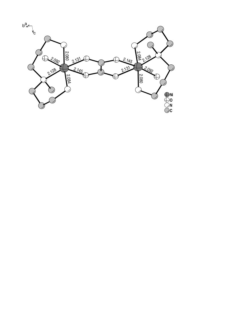
Figure 4: The homodinuclear complex cation [Ni₂(Medpt)₂($\mu$-ox)(H₂O)₂]²⁺ constituting the dinuclear core of NAOC coordination compound. This figure was drawn using the DIAMOND programme [18].

represents a centrosymmetric unit with an inversion center at the midpoint of the bridging oxalate group. This has far-reaching consequences on possible sources of the magnetic anisotropy. The antisymmetric Dzialoshinskii-Moriya interaction [19] must be entirely disregarded due to a presence of the inversion center and moreover, our previous study has revealed the totally negligible exchange anisotropy (i.e. the anisotropy in a symmetric pseudodipolar interaction) as well [9]. The most crucial contribution to the overall magnetic anisotropy should be therefore related to the single-ion anisotropy, which is closely connected to the crystal field of ligands surrounding the paramagnetic nickel centres. Altogether, the structural data listed in Fig. 4 might indicate a relatively strong uniaxial single-ion anisotropy due to a rather high difference between bond lengths to the axial and equatorial ligands, respectively. Besides, somewhat smaller biaxial single-ion anisotropy might be also expected on account of diverse bond distances in the equatorial plane. Actually, the bond distance to the coordinated water molecule is slightly shorter than the bond distances to other three equatorial ligands.

The high-field magnetization data measured in a pulsed magnetic field, which is oriented either along the crystallographic $a$- or $c^{\star}$-axis ($a\perp c^{\star}$), are plotted in Figs. 5 and 6 together with the corresponding theoretical predictions for

Figure 5: The high-field magnetization curves measured at sufficiently low temperature ($T$=1.3K) in the magnetic field applied along the crystallographic $a$- and $c^{*}$-axis, respectively. The best simultaneous fit of both these magnetization curves has been achieved through this unique set of fitting parameters: $J/k_{\rm B}=30.7$K, $D/k_{\rm B}=-12.5$K, and $g=2.26$. Both magnetization curves are displayed within the same scale in the insert of Fig. 5a in order to show a substantial anisotropy in the magnetization process.

the longitudinal and transverse magnetization. Fig. 5 shows the best simultaneous fit of both experimental magnetization curves by considering only the parameters $J$, $D$, and $g$ pertinent to a strength of the exchange interaction, uniaxial single-ion anisotropy, and gyromagnetic ratio, respectively, as the adjustable fitting parameters and neglecting the biaxial single-ion anisotropy as a higher-order anisotropy term. Even under this restriction, the results obtained from the exact numerical diagonalization directly remove ambiguity in determining a strength of the uniaxial single-ion anisotropy, which otherwise occurs in an attempt to fit both magnetization curves through a single expression for the longitudinal magnetization known from the exact analytical diagonalization (see for details Ref. [9]). According to this plot, the crystallographic $a$-, $b$- and $c^{\star}$-axes definitely turn out to be the $x$-, $y$- and $z$-axes of the effective spin Hamiltonian (1) and the negative sign of the parameter $D$ is also consistent with the experimental observation that the $c^{\star}$-axis is the easy magnetization axis [11]. The best result of a more comprehensive fitting procedure, which includes the parameter $E$ to the set of adjustable fitting parameters, is depicted in Fig. 6.

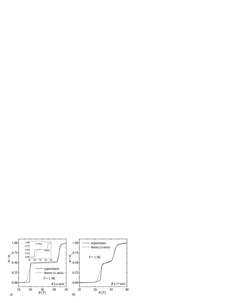
Figure 6: The high-field magnetization curves measured at sufficiently low temperature ($T$=1.3K) in the magnetic field applied along the crystallographic $a$- and $c^{*}$-axis, respectively. The best simultaneous fit of both these magnetization curves has been achieved through this unique set of fitting parameters: $J/k_{\rm B}=30.2$K, $D/k_{\rm B}=-11.0$K, $E/k_{\rm B}=1.5$K, and $g=2.20$.

Evidently, the inclusion of the parameter of biaxial single-ion anisotropy merely causes a small reduction of the most dominant interaction parameters $J$, $D$, $g$ (cf. the fitting data sets listed in the last two figure captions) and beside this, the fitting data set presented in Fig. 6 is in an excellent agreement with the one proposed by the analysis of high-field ESR data [11]. Both these facts clearly demonstrate adequate reliability and plausibility of the data sets to be obtained by fitting. When comparing the accuracy of both fitting sets in reproducing the experimental data, the latter data set fits magnetization curves more precisely in the region of intermediate magnetization plateau and around the second transition field, while the former one gives a more adequate description in a vicinity of the first transition field that is slightly underestimated in the latter fitting set. It is worthwhile to remark, however, that the magnetization curves measured in a pulsed magnetic field are not absolutely isothermal ones on behalf of a magnetocaloric effect that cools down spin system in a field ascending process close to the transition fields. This fact might be regarded as a possible reason for slightly sharper dependence of the experimental magnetization curves to be observed especially near the first transition field. Finally, it is quite plausible to argue that the actual fitting set should be capable of rendering the overall angular dependence of transition fields. Namely, this kind of fitting would represent perhaps the most efficient way how to obtain indisputable fitting set, because there is still a certain danger of overinterpretation when attempting to fit two magnetization curves through four adjustable fitting parameters. The fitting of the overall angular dependence of transition fields is nevertheless a rather time-consuming numerical problem, which is left as a challenging task for our future work.

5 Conclusion

The present article provides a deeper insight into the magnetization process of the spin-1 Heisenberg dimer model with either uniaxial or biaxial single-ion anisotropy. The main motivation to investigate this rather simple quantum spin model bears a close relationship with the fact that it serves as a versatile model for a large number of existing dinuclear coordination compounds containing the dinickel core. Within the framework of the exact numerical diagonalization method, we have constructed for the homodinuclear nickel(II) complexes essentially exact ground-state phase diagrams in the form of transition field vs. single-ion anisotropy dependence (Figs. 2 and 3). The most important finding to emerge from the present study is closely associated with a theoretical prediction concerning the possible breakdown of intermediate magnetization plateau. If the uniaxial single-ion anisotropy is strong enough with respect to the exchange interaction, we have found convincing evidence that a presence of the intermediate magnetization plateau in the applied longitudinal field demands its absence in the applied transverse field and vice versa. Owing to this fact, it could be concluded that a sufficiently strong uniaxial single-ion anisotropy (regardless of whether easy-axis or easy-plane type) is responsible for a striking magnetization process, which is characterized by two qualitatively different magnetization curves (to be obtained for two mutually orthogonal directions of the applied magnetic field) with and without the intermediate magnetization plateau.

The obtained theoretical results were also compared with the high-field magnetization measurements on the homodinuclear nickel(II) coordination compound NAOC, which is being regarded as a typical experimental realization of the spin-1 Heisenberg dimer model. The best simultaneous fit of magnetization data, which were measured in the magnetic field applied along two mutually orthogonal crystallographic $a$- and $c^{\star}$-axes, was attained for the fitting set $J/k_{\rm B}=30.2$K, $D/k_{\rm B}=-11.0$K, $E/k_{\rm B}=1.5$K, $g=2.2$ that is consistent with the one reported on previously by the analysis of high-field ESR data [11]. The actual value of the relative ratio $D/J\cong-0.36$ implies for NAOC compound a relatively strong uniaxial single-ion anisotropy of the easy-axis type, which is, on the other hand, too small to cause the breakdown of intermediate magnetization plateau theoretically predicted (the threshold value is $D_{\rm l}/J=-0.67$). From this point of view, high-field magnetization measurements on another single-crystal samples prepared from an immense reservoir of homodinuclear nickel(II) complexes [9] would be desirable in order to provide an experimental confirmation of this interesting quantum phenomenon. Even though a design of molecule-based magnetic materials with a tunable strength of the exchange interaction and single-ion anisotropy is far from being a routine target at present, the homodinuclear nickel(II) complexes with a less rigid bridging group (i.e. with a possibly weaker exchange interaction) and simultaneously a higher distortion of coordination octahedron (i.e. with a possibly stronger single-ion anisotropy) might be considered as suitable candidates for displaying such an interesting quantum phenomenon.

References

- [1] R. D. L. Carlin, Magnetochemistry, Springer, Berlin, 1986; R. D. Willett, D. Gatteschi, O. Kahn, Magneto-Structural Correlations in Exchange Coupled Systems, vol. C140, Reidel, Dordrecht, 1985; O. Kahn, Molecular Magnetism, VCH, Weinheim, 1993; D. Gatteschi, O. Kahn, J. S. Miller, F. Palacio, Magnetic Molecular Materials, vol. E198, Kluwer, Dordrecht, 1999; K. Itoh, M. Kinoshita, Molecular Magnetism, New Magnetic Materials, Kodaisha, Tokyo, 2000; P. G. Lacroix, Chem. Mat. 13 (2001) 3495.
- [2] O. Sato, T. Iyota, A. Fujijishima, K. Hashimoto, Science 272 (1996) 704; K. Inoue, K. Kikuchi, M. Ohba, H. Ōkawa, Angew. Chem. Int. Ed. 42 (2003) 4810; S. Ohkoshi, H. Tokoro, K. Hashimoto, Coord. Chem. Rev. 249 (2005) 1830; Y. Einaga, J. Photoch. Photobio. C 7 (2006) 69.
- [3] R. Sessoli, D. Gatteschi, A. Caneschi, M. A. Novak, Nature 365 (1993) 141; C. P. Landee, D. Melville, J. S. Miller, in Magnetic Molecular Materials, edited by D. Gatteschi, O. Kahn, J. S. Miller, Kluwer, Dordrecht, 1991.
- [4] M. Leuenberger and D. Loss, Nature 410 (2001) 789.
- [5] Y. Shapira and V. Bindilatti, J. Appl. Phys. 92 (2002) 4155.
- [6] D. Gatteschi, R. Sessoli, Angew. Chem. Int. Ed. 42 (2003) 268; D. Gatteschi, A. L. Barra, A. Caneschi, A. Cornia, R. Sessoli, L. Sorace, Coord. Chem. Rev. 250 (2006) 1514; D. Gatteschi, R. Sessoli, J. Villain, Molecular Nanomagnets, Oxford University Press, Oxford, 2006.
- [7] R. Clérac, H. Miyasaka, M. Yamashita, C. Coulon, J. Am. Chem. Soc. 124 (2002) 12837; H. Miyasaka, R. Clérac, K. Mizushima, K. Sugiura, M. Yamashita, W. Wernsdorfer, C. Coulon, Inorg. Chem. 42 (2003) 8203; C. Coulon, R. Clérac, L. Lecren, W. Wernsdorfer, H. Miyasaka, Phys. Rev. B 69 (2004) 132408; R. Lescouëzec, L. M. Toma, J. Vaissermann, M. Verdaguer, F. S. Delgado, C. Ruiz-Pérez, F. Lloret, M. Julve, Coord. Chem. Rev. 249 (2005) 2691; H. Miyasaka, R. Clérac, Bull. Chem. Soc. Jpn. 78 (2005) 1725; C. Coulon, H. Miyasaka, R. Clerac, Structure and Bonding 122 (2006) 163.
- [8] O. Kahn, Phil. Trans. R. Soc. Lond. A 357 (1999) 3005; G. L. Abbati, L. C. Brunel, H. Casalta, A. Cornia, A. C. Fabretti, D. Gatteschi, A. K. Hassan, A. G. M. Jansen, A. L. Maniero, L. Pardi, C. Paulsen, Chem. Eur. J. 7 (2001) 1796; D. Gatteschi, L. Sorace, J. Solid St. Chem. 159 (2001) 253; J. van Slageren, R. Sessoli, D. Gatteschi, A. A. Smith, M. Helliwell, R. E. P. Winpenny, A. Cornia, A. L. Barra, A. G. M. Jansen, E. Rentschler, G. A. Timco, Chem. Eur. J. 8 (2002) 277; R. Boča, Coord. Chem. Rev. 248 (2004) 747; D. V. Efremov, R. A. Klemm, Phys. Rev. B 74 (2006) 064408.
- [9] J. Strečka, M. Jaščur, M. Hagiwara, Y. Narumi, J. Kuchár, S. Kimura, K. Kindo, J. Phys. Chem. Solids 66 (2005) 1828.
- [10] Y. Narumi, R. Sato, K. Kindo, M. Hagiwara, J. Magn. Magn. Mater. 177-181 (1998) 685.
- [11] S. Kimura, S. Hirai, Y. Narumi, K. Kindo, M. Hagiwara, Physica B 294-295 (2001) 47.
- [12] H. T. Wittenveen, W. L. C. Rutten, J. Reedjick, J. Inorg. Nucl. Chem. 37 (1975) 913; A. Vermas, W. Z. Groeneveld, J. Reedjick, Z. Naturforsch. Teil A 32 (1977) 632; R. L. Carlin, L. J. de Jongh, Chem. Rev. 86 (1986) 659; G. DeMunno, M. Julve, F. Lloret, A. Derory, J. Chem. Soc. Dalton Trans. (1993) 1179.
- [13] O. Kahn, Structure and Bonding 68 (1987) 89; J. H. Satcher, M. W. Droege, T. J. R. Weakley, R. T. Taylor, Inorg. Chem. 34 (1995) 3317.
- [14] A. Earnshaw, B. N. Figgis, J. Lewis, J. Chem. Soc. A (1966) 1656.
- [15] A. P. Ginsberg, Inorg. Chim. Acta Rev. 5 (1971) 45; A. P. Ginsberg, R. L. Martin, R. W. Brookes, R. C. Sherwood, Inorg. Chem. 11 (1972) 2884.
- [16] http://www.netlib.org/lapack/
- [17] A. Escuer, R. Vicente, J. Ribas, J. Jaud, B. Raynaud, Inorg. Chim. Acta 216 (1994) 139.
- [18] DIAMOND Visual Crystal Structure Information System, Crystal Impact D-53002 Bonn, Germany, 1999.
- [19] I. Dzialoshinskii, J. Phys. Chem. Solids 4 (1958) 241; T. Moriya, Phys. Rev. Lett. 4 (1960) 5; T. Moriya, Phys. Rev. 120 (1960) 91.