Euler equation of the optimal trajectory for the fastest magnetization reversal of nano-magnetic structures

Abstract

Based on the modified Landau-Lifshitz-Gilbert equation for an arbitrary Stoner particle under an external magnetic field and a spin-polarized electric current, differential equations for the optimal reversal trajectory, along which the magnetization reversal is the fastest one among all possible reversal routes, are obtained. We show that this is a Euler-Lagrange problem with constrains. The Euler equation of the optimal trajectory is useful in designing a magnetic field pulse and/or a polarized electric current pulse in magnetization reversal for two reasons. 1) It is straightforward to obtain the solution of the Euler equation, at least numerically, for a given magnetic nano-structure characterized by its magnetic anisotropy energy. 2) After obtaining the optimal reversal trajectory for a given magnetic nano-structure, finding a proper field/current pulse is an algebraic problem instead of the original nonlinear differential equation.

The advent of miniaturization and fabrication of magnetic particles with single magnetic domainsQikun , called Stoner particles, makes the Stoner-Wohlfarth (SW) problembook very relevant to nano-technologies and nano-sciences. One current topic in nanomagnetism is the controlled manipulation of magnetization dynamics of Stoner particles. Magnetization state can be manipulated by a magnetic fieldfield ; xrw ; xrw1 through the usual magnetization-field interaction, or by a spin-polarized electric currentSlon ; theory ; three ; exp ; zhang ; sun ; xrw2 through the so-called spin-transfer torque (STT), or by a laser lightBigot . In terms of applications, controlled manipulation of a magnetization by a magnetic field and/or a spin-polarized electric current is and would be dominating techniques in information storage industry. The magnetization dynamics of a Stoner particle under the influence of a magnetic field and/or a spin-polarized current is described by the so-called nonlinear Landau-Lifshitz-Gilbert (LLG) equation that does not have analytical solutions. Most of the results obtained so far on magnetization reversal are either from a numerical solutionfield of a given field/current pulse or based on a specific featuresun ; xrw ; zhang of the LLG equation. Important issues are to lower critical fields/currents required to reverse a magnetizationsun and to design a field/current pulse such that the magnetization can be switched from one state to another as quickly as possiblexrw1 ; xrw2 .

Many reversal schemessun ; xrw ; zhang have been proposed and examined. To evaluate different reversal schemes, it is important to know the theoretical limits of the critical switching field/current, and the optimal field/current pulse for the fastest magnetization reversal. The answers to the above questions were only known recently for the simplest Stoner particles of uniaxial magnetic anisotropy when either a magnetic field or a spin-polarized electric currentxrw1 ; xrw2 is used to reverse the magnetization. Unfortunately, those ideas and approaches, based on the rotational symmetry of the system around its easy-axes, are not applicable to a non-uniaxial Stoner particle. In fact, the method does not even work on an uniaxial Stoner particle reversed by a spin-polarized electric current and a static magnetic field non-collinear to its easy-axis, a possible useful model in current-controlled MRAM (magnetic random access memory) devices. The solutions (answers) of these questions for an arbitrary Stoner particle under combined influences of a magnetic field and an electric current are the themes of current work. In this letter, the Euler equation of the optimal reversal trajectory is derived. For the special case of reversal of uniaxial Stoner particles by either a magnetic field or a Slonczewski-type of STT, analytical solution of the equation can be obtained, which accord with the early results in References 5 and 12. In general, the equation can be numerically solved easily for a given Stoner particle of a known magnetic anisotropy energy. Given a reversal trajectory, finding the required field/current pulse is an algebraic problem. The generality of the current theory is demonstrated on a biaxial Stoner particle.

Consider a Stoner particle of a magnetization $\vec{M}=M\vec{m}$ under the influence of an external magnetic field $\vec{H}$ as well as a polarized electric current of $I$, where $M$ is the saturated magnetization of the particle and $\vec{m}$ is the unit vector of $\vec{M}$. Theoretical studiesSlon ; theory ; three show that the STT $\Gamma$ is proportional to the current with following form

$$\Gamma\equiv[\frac{d(\vec{M}V)}{dt}]_{STT}=\frac{\gamma\hbar I}{\mu_{0}e}g(P,\vec{m}\cdot\hat{s})\vec{m}\times(\vec{m}\times\hat{s}),$$

where $\hat{s}$ is the polarization direction of the current. In the expression, $V$, $\hbar$, $\mu_{0}$($=4\pi\times 10^{-7}N/A^{2}$), and $e$ denote the volume of the magnetic nano-structure, the Planck constant, the vacuum magnetic permeability, and the electron charge, respectively. $\gamma=2.21\times 10^{5}(rad/s)/(A/m)$ is the gyromagnetic ratio. The exact microscopic formulation of STT is still a debating subjecttheory ; three . Most of existing theories differ themselves in different $g$-functions that depend on the degree of the polarization $P$ of the current and relative angle between $\vec{m}$ and $\hat{s}$. Many experimental investigationsexp so far are consistent with the result of SlonczewskiSlon , $g=4P^{3/2}/[(1+P)^{3}(3+\vec{m}\cdot\hat{s})-16P^{3/2}]$, which will be assumed in this study whenever we need an explicit expression of $g$.

The dynamics of the magnetization $\vec{M}$ is governed by the generalized LLG equationxrw2 ,

$$\frac{d\vec{M}}{dt}=-\gamma\vec{M}\times\vec{H}_{t}+\alpha\vec{m}\times\frac{d\vec{M}}{dt}+\gamma a_{I}\vec{M}\times(\vec{M}\times\hat{s}),$$ (1)

where $\alpha$ is the phenomenological dimensionless damping constant and $a_{I}=\hbar Ig/(\mu_{0}eM^{2}V)$ is a dimensionless parameter of Slonczewski STTSlon . $\vec{H}_{t}$ is the usual total effective magnetic field. Notice that $M$ is a constant according to Eq. (1), it is convenient to re-write the LLG equation in the dimensionless form,

$$(1+\alpha^{2})\frac{d\vec{m}}{dt}=-\vec{m}\times\vec{h}_{1}-\vec{m}\times(\vec{m}\times\vec{h}_{2}),$$ (2)

where $\vec{h}_{1}=\vec{h}_{t}+\alpha a_{I}\hat{s},$ and $\vec{h}_{2}=\alpha\vec{h}_{t}-a_{I}\hat{s}$. $t$ in Eq. (2) is in the units of $(\gamma M)^{-1}$. Both magnetization and magnetic field are in the units of $M$. The total field $\vec{h}_{t}\equiv\vec{H}_{t}/M=\vec{h}+\vec{h}_{i}$ includes both the applied magnetic field $\vec{h}=\vec{H}/M$ and the internal field $\vec{h}_{i}$ due to the magnetic anisotropic energy density $w(\vec{m})$, $\vec{h}_{i}=-\nabla_{\vec{m}}w(\vec{m})/\mu_{0}$. $\vec{h}_{1}$ and $\vec{h}_{2}$ are in general non-collinear, thus the dynamics with the additional STT term in Eq. (1) is quite differentxrw2 from that without this term which describes a Stoner particle in a magnetic field only: The particle energy can only decrease in a static magnetic field since the field cannot be an energy sourcexrw . However, a polarized electric current can pump energy into a Stoner particle through the STT. Thus, STT allows even a dc current to be an energy source, and dynamics and physics of a Stoner particle under a STTexp ; zhang ; sun are much richer than that under a static magnetic field. According to Eq. (2), the magnetization undergoes a precessional motion around field $h_{1}$ and a damping motion toward field $h_{2}$.

In terms of polar angle $\theta$ and azimuthal angle $\phi$ of $\vec{m}$ in the spherical coordinates, Eq. (2) becomes

$$(1+\alpha^{2})\dot{\theta}=a_{I}(\alpha s_{\phi}-s_{\theta})-\alpha(\frac{\partial w}{\partial\theta}-h_{\theta})+$$

$$\qquad\qquad\quad h_{\phi}-\frac{1}{\sin\theta}\frac{\partial w}{\partial\phi}\equiv F_{1},$$

$$(1+\alpha^{2})\sin\theta\dot{\phi}=-a_{I}(\alpha s_{\theta}+s_{\phi})-h_{\theta}+$$ (3)

$$\qquad\qquad\frac{\partial w}{\partial\theta}+\alpha(h_{\phi}-\ \frac{1}{\sin\theta}\frac{\partial w}{\partial\phi})\equiv F_{2},$$

where $\dot{f}$ means derivative of $f$ with respect to time $t$. Here $s_{r}$, $s_{\theta}$, $s_{\phi}$ are the $r,\ \theta$, and $\phi$ components of $\hat{s}$, and

$$G_{1}\equiv s_{\phi}^{2}+s_{\theta}^{2}+s_{r}^{2}-1=0.$$ (4)

Since the radial component of the external magnetic field does not appear in the dynamics equation of the magnetization. $h_{r}$ shall not affect the magnetization dynamics, and we shall always assume $h_{r}=0$ for an optimal field pulse. However, for STT induced reversal, $s_{r}$ will affect the magnetization dynamics through the STT coefficient $a_{I}$ which is a function of $P$ and $s_{r}$. In general, $F_{i},\ (i=1,2)$ are functions of $\theta,\ \phi,\ h_{\theta},\ h_{\phi},\ s_{\theta},\ s_{\phi}$, and $s_{r}$. The switching problem is as follows: Before applying a field/current, magnetization $\vec{m}$ has two stable states, $\vec{m}_{0}$ (‘north pole’ $\theta=0$) and $-\vec{m}_{0}$ (‘south pole’ $\theta=\pi)$ along its easy axis (z-axis). Initially, the particle is in state $\vec{m}_{0}$, and the goal is to use a field pulse and a spin-polarized electric current pulse to switch the magnetization to $-\vec{m}_{0}$ quickly. Both the field direction and the spin polarization direction may vary with time.

It will be beneficial to make a qualitative description of the relationships among field/current pulses, reversal trajectory, and reversal time. Given a field/current pulse, magnetization $\vec{m}$ will move following Eq. (Euler equation of the optimal trajectory for the fastest magnetization reversal of nano-magnetic structures) if $\vec{m}_{0}$ is no longer a stable state under the field/current pulse. Eventually, the system will end up at one of its new stable statesfield . If the pulse is proper, its evolution path $\phi(\theta)$ may pass through $-\vec{m}_{0}$. When that happens, the path is called a reversal trajectory, and the corresponding field/current pulses are reversal pulses. Given a reversal field/current pulse, there is a unique reversal trajectory which is the solution of Eq. (2), a nonlinear problem with no general analytic solution. However, knowing a reversal trajectory $\phi(\theta)$, which pass through $\theta=0,\pi$, there are infinite number of reversal pulses satisfying, according to Eq. (Euler equation of the optimal trajectory for the fastest magnetization reversal of nano-magnetic structures),

$$\phi^{\prime}\sin\theta F_{1}-F_{2}\equiv G_{2}=0,$$ (5)

where $\phi^{\prime}\equiv d\phi/d\theta$. All $h_{i}$ and $s_{i}$ ($i=r,\theta,\phi$) satisfying Eq. (5) form reversal pulses. Thus, there is a functional relationship between reversal pulse and reversal trajectory. What is more, given a reversal trajectory, magnetization “velocities” $\dot{\theta}$ and $\dot{\phi}$ are linear in $\vec{h}$ and $I$. In other words, the reversal time shall be monotonic in $I$ and $h$, magnitude of $\vec{h}$. As $h$ and/or $I$ approach infinity, the reversal time goes to zero. Thus, the optimization problem (shortest reversal time) is meaningful only when one imposes additional conditions on $h$ and $I$. One sensible way is to fix $I$ and $h$, i.e.,

$$G_{3}\equiv h_{\phi}^{2}+h_{\theta}^{2}-h^{2}=0.$$ (6)

According to Eq. (Euler equation of the optimal trajectory for the fastest magnetization reversal of nano-magnetic structures), the reversal time $T$ along a reversal trajectory is given by

$$T=\int_{0}^{\pi}\frac{d\theta}{\dot{\theta}}=\int_{0}^{\pi}\frac{(1+\alpha^{2})d\theta}{F_{1}}.$$ (7)

The optimization problem here is to find the optimal reversal trajectory for the fastest magnetization reversal under the constrains of Eqs. (4) and (6). Thus $T$ is minimal against the variation of the reversal trajectories $\phi(\theta)$ and field/current pulses $h_{i}$ and $s_{i}$ ($i=r,\theta,\phi$) that are linked together by Eq. (5). This is just the Euler-Lagrange problem. Using Lagrange multipliers method, the optimal reversal trajectory and optimal reversal field/current pulses are given by

$$\frac{d}{d\theta}(\frac{\partial F}{\partial\phi^{\prime}})=\frac{\partial F}{\partial\phi},$$

$$\frac{d}{d\theta}(\frac{\partial F}{\partial h_{i}^{\prime}})=\frac{\partial F}{\partial h_{i}},\qquad(i=\theta,\phi)$$

$$\frac{d}{d\theta}(\frac{\partial F}{\partial s_{i}^{\prime}})=\frac{\partial F}{\partial s_{i}},\qquad(i=r,\theta,\phi)$$ (8)

$$F=\frac{1+\alpha^{2}}{F_{1}}+\lambda_{1}G_{1}+\lambda_{2}G_{2}+\lambda_{3}G_{3},$$

$$G_{1}=0,\qquad G_{2}=0,\qquad G_{3}=0,$$

where ${}^{\prime}=\frac{d}{d\theta}$, thus, $f^{\prime}$ means derivative of $f$ with respect to $\theta$. $\lambda_{1,2,3}$ are the Lagrange multipliers that can be determined self-consistently from Eqs. (Euler equation of the optimal trajectory for the fastest magnetization reversal of nano-magnetic structures).

Eqs. (Euler equation of the optimal trajectory for the fastest magnetization reversal of nano-magnetic structures) are the central result of the current work. For a given $I$, $P$, $h$, and particle ($w(\vec{m})$ is known), the solution of the equations yield the optimal reversal trajectory $\phi(\theta)$ and optimal reversal field/current pulse $h_{i}$ and $s_{i}$ ($i=r,\theta,\phi$). Knowing the information, it is a straightforward task to find the theoretical limit of minimum switching field/current. Obviously, one can simultaneously optimize the field and the current in a controlled manipulation. From an application point of view, such a set up could be complicate and expensive, and one may be more interested in using one means only, i.e. either a field or a current, to manipulate a magnetization. Two cases may be interesting. Case A): Fix $I$ and $\hat{s}$, and vary $h_{\theta}$ and $h_{\phi}$. Reference 5 is a special example of the case with $I=0$. Case B): Fix the magnetic field $\vec{h}$ and the magnitude of current $I$, and vary the current polarization. Reference 12 is a special example ($\vec{h}=0$) of the case.

In order to demonstrate that Eq. (Euler equation of the optimal trajectory for the fastest magnetization reversal of nano-magnetic structures) is capable to find the optimal reversal trajectory for an arbitrary Stoner particle, let us consider case A), magnetic field induced magnetization reversal, $a_{I}=0$. After some tedious and straightforward calculation, the Euler equations become

$$\frac{\partial^{2}L}{\partial\phi^{\prime 2}}\phi^{\prime\prime}+\frac{\partial^{2}L}{\partial\phi\partial\phi^{\prime}}\phi^{\prime}+\frac{\partial^{2}L}{\partial\theta\partial\phi^{\prime}}-\frac{\partial L}{\partial\phi}=0,$$

$$f_{1}=\frac{\partial w}{\partial\theta}-\frac{\alpha}{\sin\theta}\frac{\partial w}{\partial\phi};\quad f_{2}=-\alpha\frac{\partial w}{\partial\theta}-\frac{1}{\sin\theta}\frac{\partial w}{\partial\phi},$$

$$L=\frac{\phi^{\prime}\sin\theta f_{1}+f_{2}}{f_{1}^{2}+f_{2}^{2}-(1+\alpha^{2})h^{2}}\pm$$ (9)

$$\frac{\sqrt{(1+\phi^{\prime 2}\sin^{2}\theta)(1+\alpha^{2})h^{2}-(f_{1}-\phi^{\prime}\sin\theta f_{2})^{2}}}{f_{1}^{2}+f_{2}^{2}-(1+\alpha^{2})h^{2}},$$

where $f_{1,2}$ are functions of $\theta$ and $\phi$ determined by magnetic anisotropy energy $w(\vec{m})$. $w=-km_{z}^{2}/2$ corresponds to References 5, and it can be shown that Eqs. (Euler equation of the optimal trajectory for the fastest magnetization reversal of nano-magnetic structures) is

$$\phi^{\prime}=\frac{2\cos\theta}{\alpha(h/h_{c}-\sin 2\theta)}.$$ (10)

Its solution is

$$\phi=\phi_{0}+\frac{1}{\alpha}\sqrt{\frac{h_{c}}{h-h_{c}}}\arctan[\sqrt{\frac{2h_{c}}{h-h_{c}}}\sin(\theta-\frac{\pi}{4})]+$$

$$\frac{\sqrt{h_{c}}}{2\alpha\sqrt{h+h_{c}}}\ln\frac{\sqrt{(h/h_{c}+1)/2}+\cos(\theta-\frac{\pi}{4})}{\sqrt{(h/h_{c}+1)/2}-\cos(\theta-\frac{\pi}{4})},$$

where $\phi_{0}$ is an arbitrary constant reflecting the $\phi-$ symmetry of the system. This is exactly the same optimal trajectory equation obtained in Reference 5 with the theoretical limit of switching field being $h_{c}=max\{\alpha k\cos\theta\sin\theta/\sqrt{1+\alpha^{2}}\}=\alpha k/(2\sqrt{1+\alpha^{2}})$. All other results in Reference 5 can be re-derived from this optimal reversal trajectory.

For a biaxial Stoner particle of $w(\theta,\phi)=-(k_{1}/2)\cos^{2}\theta+(k_{2}/2)\sin^{2}\theta\cos^{2}\phi$, Eq.(Euler equation of the optimal trajectory for the fastest magnetization reversal of nano-magnetic structures) may not be easy to solve analytically, but numerical solutions are easy to find. The solutions for $\alpha=0.1$, $k_{1}=1$, and $h=1(\gg h_{c}$, which is about 0.05 for $k_{2}=0$) are presented in Fig. 1 for $k_{2}=0,1,5,10$, respectively. Fig. 1a shows the optimal trajectories. It is interesting to note that the optimal trajectories for $k_{2}=0$ has rotational symmetry around z-axis (an infinite number of solutions). The one shown in Fig. 1a is just a particular solution with $\phi(t=0)=0$. For $k_{2}\neq 0$, the rotational symmetry is broken, but there are still four equivalent trajectories due to the biaxial symmetry. The ones whose inital $\phi$’s are in the range of $[0,\pi/2]$ are used in the figure. Fig. 1b and 1c are the time evolution of $\theta$ and $\phi$ along the trajectories. It is surprising to note that switching time is shorter and shorter as $k_{2}$ increases, and the potential landscape is less smooth. Fig. 1d and 1e are the corresponding optimal reversal pulses.

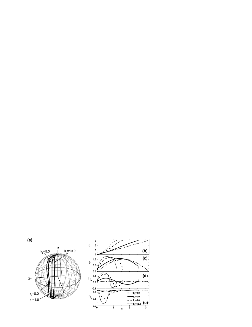
Figure 1: Numerical solutions of biaxial model with $\alpha=0.1$, $k_{1}=1$, $h=1$, and various $k_{2}=0,1,5,10$. a) The optimal reversal trajectories. b) $\theta$ vs. $t$. c) $\phi$ vs. t. d) $h_{\theta}$ vs. t. e) $h_{\phi}$ vs. t.

Similarly, one can obtain all the results in Reference 12 from Eqs. (Euler equation of the optimal trajectory for the fastest magnetization reversal of nano-magnetic structures). Only a spin-polarized current is used to manipulate the magnetization reversal of a uniaxial Stoner particle there, and the system specifities are $\vec{h}=0$, $I=const.,$ $P=const.$, and $w=w(\cos\theta)$ with $-\partial w/\partial(\cos\theta)\equiv f(\cos\theta)$. After some algebras, the optimal trajectory equation is

$$\phi^{\prime}==\frac{f(\cos\theta)}{\alpha Q[I/I_{c}-f(\cos\theta)\sin\theta/Q]},$$ (11)

where $I_{c}=\frac{\mu_{0}eM^{2}V}{\hbar G(P)}\frac{\alpha}{\sqrt{1+\alpha^{2}}}Q$ is the theoretical limit of the critical switching current, $Q\equiv max\{f(\cos\theta)\sin\theta\}$ for $\theta\in[0,\pi]$ depends on the magnetic anisotropy energy landscape, and $G(P)=g(P,s_{r}^{*})\sqrt{1-s_{r}^{*2}}$ comes from the $g$-function in Slonczewski STT. The corresponding optimal polarization pulse is given by

$$s_{r}^{*2}=\frac{(1+P)^{3}}{16P^{3/2}-3(1-P)^{3}},$$

$$s_{\phi}^{*2}=-\alpha s_{\theta}^{*2}=\frac{\alpha}{\sqrt{1+\alpha^{2}}}\sqrt{1-s_{r}^{*2}}.$$ (12)

The trajectory equation has exactly the same form as that of magnetic-field case, reflecting the fact that both cases are described by the same dynamical equation (2). These are exactly what were found in Reference 12 from a special observation.

Our derivation of the Euler equation is based on the following observations. 1) Given a field/current pulse on a macro-spin of a magnetic nano-structure, the trajectory of its magnetization is uniquely determined by the corresponding LLG equation (Euler equation of the optimal trajectory for the fastest magnetization reversal of nano-magnetic structures). 2) Knowing a reversal trajectory $\phi(\theta)$ (not $\theta(t)$ and $\phi(t)$ ), there are an infinite number of possible pulses, satisfying condition (5), that can reverse the magnetization along the trajectory. 3) The issue of the optimal magnetization reversal trajectory is an Euler-Lagrange problem with constrains.

The Euler equation is more useful than the LLG equation in designing an optimal field/current pulse, although the Euler equation is derived from the later one. With only a LLG equation, one can only determine one magnetization trajectory for one specific field/current pulse. Thus, one does not even know whether the pulse can reverse a magnetization! Before obtaining all solutions of all possible pulses, one would not be able to tell which one is the best. With the Euler equation, one can obtain the optimal reversal trajectory and reversal pulses directly for a given particle. It should be pointed out that the current work address the same issues as those in References 5 and 12, but it provides a general and unified theory which can deal with combined effects of a field and a current for an arbitrary Stoner particle.

In conclusion, a unified theory for the optimal magnetization reversal trajectories and reversal field and/or current pulses of an arbitrary Stoner particle is presented. The theory provides the Euler equation of the optimal reversal trajectory along which the magnetization reversal is the fastest is derived. Our early results on the critical switching field/current for a unixial Stoner particle are reproduced with the unified theory. The optimal magnetization reversal of a biaxial Stoner particle is also solved.

Acknowledgments–This work is supported by UGC, Hong Kong, through RGC CERG grants (#603106 and #603007).

References

- (1) M.H. Pan, H. Liu, J.Z. Wang, J.F. Jia, Q.K. Xue, J.L. Li, S. Qin, U.M. Mirdaidov, X.R. Wang, J.T. Market, Z.Y. Zhang, and C.K. Shih, Nano Letters 5, 87(2005).
- (2) B. Hillebrands and K. Ounadjela, eds., Spin Dynamics in Confined Magnetic Structures I & II, (Springer-Verlag, Berlin, 2001).
- (3) L. He, and W.D. Doyle, IEEE. Trans. Magn. 30, 4086 (1994); Y. Acremann, C.H. Back, M. Buess, O. Portmann, A. Vaterlaus, D. Pescia, and H. Melchior, Science 290, 492 (2000); Z.Z. Sun, and X.R. Wang, Phys. Rev. B 71, 174430 (2005).
- (4) Z.Z. Sun, and X.R. Wang, Phys. Rev. B 73, 092416 (2006); 74, 132401 (2006).
- (5) Z.Z. Sun, and X.R. Wang, Phys. Rev. Lett. 97, 077205 (2006).
- (6) J. Slonczewski, J. Magn. Magn. Mater. 159, L1 (1996); L. Berger, Phys. Rev. B 54 9353 (1996).
- (7) J.Z. Sun, Phys. Rev. B 62, 570 (2000); Z. Li and S. Zhang, ibid. 68, 024404 (2003); Y.B. Bazaliy, B.A. Jones and S.C. Zhang, ibid. 57, R3213 (1998); 69, 094421 (2004).
- (8) A. Brataas, Y.V. Nazarov, and G.E.W. Bauer, Phys. Rev. Lett. 84, 2481 (2000); X. Waintal, E.B. Myers, P.W. Brouwer, and D.C. Ralph, Phys. Rev. B 62, 12317 (2000); M.D. Stiles, A. Zangwill, ibid. 66, 014407 (2002).
- (9) M. Tsoi, A. G. M. Jansen, J. Bass, W.-C. Chiang, M. Seck, V. Tsoi, and P. Wyder, Phys. Rev. Lett. 80, 4281 (998); E.B. Myers, D.C. Ralph, J.A. Katine, R. N. Louie, and R.A. Buhrman, Science 285, 867 (1999); J.A. Katine, F.J. Albert, R.A. Buhrman, E.B. Myers, and D.C. Ralph, Phys. Rev. Lett. 84, 3149 (2000).
- (10) Z. Li and S. Zhang, Phys. Rev. B 69, 134416 (2004); W. Wetzels, G.E.W. Bauer, and O.N. Jouravlev, Phys. Rev. Lett. 96, 127203 (2006).
- (11) J. Sun, J. Magn. Magn. Mater. 202, 157 (1999); Nature 425, 359 (2003); K.J. Lee, O. Redon, and B. Dieny, Appl. Phys. Lett. 86, 022505 (2005); J. Manschot, A. Brataas, and G.E.W. Bauer, ibid. 85, 3250 (2004); A.D. Kent, B. Özyilmaz, and E. del Barco, ibid. 84, 3897 (2004); T. Moriyama, R. Cao, J.Q. Xiao, J. Lu, X.R. Wang, Q. Wen, and H.W. Zhang, ibid. 90, 152503 (2007).
- (12) X.R. Wang, and Z.Z. Sun, Phys. Rev. Lett. 98, 077201 (2007).
- (13) M. Vomir, L.H.F. Andrade, L. Guidoni, E. Beaurepaire, and J.-Y. Bigot, Phys. Rev. Lett. 94, 237601 (2005).
- (14) R.H. Koch, J.A. Katine, and J.Z. Sun, Phys. Rev.Lett. 92, 088302 (2004).
- (15) X. Wang, G.E.W. Bauer, and A. Hoffmann, Phys. Rev. B 73, 054436 (2006).