Chaotic oscillations in a map-based model of neural activity

Abstract

We propose a discrete time dynamical system (a map) as phenomenological model of excitable and spiking-bursting neurons. The model is a discontinuous two-dimensional map. We find condition under which this map has an invariant region on the phase plane, containing chaotic attractor. This attractor creates chaotic spiking-bursting oscillations of the model. We also show various regimes of other neural activities (subthreshold oscillations, phasic spiking etc.) derived from the proposed model.

The observed types of neural activity are extremely various. A single neuron may display different regimes of activity under different neuromodulatory conditions. A neuron is said to produce excitable mode if a ”superthreshold” synaptic input evokes a post-synaptic potential in form of single spikes, which is an order of magnitude larger than the input amplitude. While a ”subthreshold” synaptic input evokes post-synaptic potentials of the same order. Under some conditions a single spike can be generated with arbitrary low frequency, depending on the strength of the applied current. It is called spiking regime. An important regime of neural activity is bursting oscillations where clusters of spikes occur periodically or chaotically, separated by phases of quiescence. Other important observed regimes are phasic spikes and bursts, subtreshold oscillations and tonic spiking. Understanding dynamical mechanisms of such activity in biological neurons has stimulated the development of models on several levels of complexity. To explain biophysical membrane processes in a single cell, it is generally used ionic channel-based models b:Kandel . The prototype of those models is the Hodgkin-Huxley system which was originally introduced in the description of the membrane potential dynamics in the giant squid axon. This is a high dimensional system of nonlinear partial differential equations. Another class of neuron models are the phenomenological models which mimic qualitatively some distinctive features of neural activity with few differential equations. For example, the leaky integrate-and-fire model, Hindmarsh-Rose and FitzHugh-Nagumo model etc. A new important subclass of phenomenological models is the map-based systems. Basically such models are designed with the aim of simulating collective dynamics of large neuronal networks. The map-based models possess at least the same features of Ordinary differential equations (ODE) models, and have more simple intrinsic structure offering an advantage in describing more complex dynamics. In order to model basic regimes of neural activity we design new family of maps that are two-dimensional and based on discrete FitzHugh-Nagumo system in which we introduce Heaviside step function. The discontinuity line determines the excitation threshold of chaotic spiking-bursting oscillations. For some domain of the parameters, we found on phase plane an invariant bounded region containing chaotic attractor with spiking-bursting activity. The interesting fact is that the dynamical mechanism, leading to chaotic behavior of our two-dimensional map is induced by one-dimensional Lorenz-like map. We demonstrate also that our model can display rich gallery of regimes of neural activity such as chaotic spiking, subthreshold oscillations, tonic spiking etc.All these modes play important role in the information processing in neural systems.

I Introduction

The nervous system is an extremely complex system b:Kandel comprising nerve cells (or neurons) and gial cells. By electrical and chemical synapses of different polarity neurons form a great variety large-scale networks. Therefore, modeling of brain’s key functional properties is associated with study of collective activity of complex neurobiological networks. Dynamical modeling approach b:Rabinovich is effective tool for the analysis of this kind of networks. First of all this approach takes building dynamical models of single neurons. On the one hand, such models should describe large quantity of various dynamical modes of neural activity (excitable, oscillatory, spiking, bursting, etc.). This complexity is associated with the large number of voltage-gated ion channels of neurons. It takes employment of complex nonlinear dynamical systems given by differential equations. The canonical representative of this type of models is Hodgkin-Huxley system. It describes dynamics of the transport through membrane of neuron in detail. On the other hand, to model neural network consisting of the large number of interconnected units it is necessary to create simplified models for single neuron to avoid problems that are induced by high dimension and nonlinearity. For example, one which is commonly used in simulations is integrate-and-fire model b:IandFModel . It represents one-dimensional nonlinear equation with some threshold rule. That is, if the variable of the model crosses a critical value, then it is reset to new value and the neuron is said to have fired. To solve the contradiction between the requirements of complexity and simplicity of neuron models phenomenological models were introduced. They describe basic properties of neuron dynamics, but these models do not take into account the large number of voltage-gated ion channels of neurons. As a rule they involve generalized variable which mimic the dynamic of some number of ionic currents at the same time. The examples of this type models are FitzHugh-Nagumo b:FitzHugh , Hindmarsh-Rose b:HingmarshRose , Morris-Lecar b:MorrisLekar . They have the form of differential equations systems. However, there is another class of phenomenological models of the neural activity. These are discrete-time models in form of point maps. In the last decade this kind of neural models has attracted much attentionb:Chialvo ; b:Kinouchi ; b:Kuva ; b:DeVries . For example using a map-based approach Rulkov et. al. b:RulkovTim have studied dynamics of one- and -two dimensional large-scale cortical networks. It has been found that such map-based models produce spatiotemoral regimes similar to those exhibited by Hodgkin-Huxley -like models.

Neuron oscillatory activity can take a variety of forms b:Traub . One of the most interesting oscillatory regimes is spiking-bursting oscillations regime, which is commonly observed in a wide variety of neurons such as hippocampal pyramidal neurons, thalamic neurons, pyloric dilator neurons etc. A burst is a series of three or more action potential usually riding on a depolarizing wave. It is believed that the bursting oscillations play crucial role in informational transmitting and processing in neurons, facilitate secretion of hormones and drive a muscle contraction. This oscillation can be regular or chaotic depending on the concentration of neuromodulators, currents and other control parameters. Another interesting oscillatory regime is an oscillation of membrane potential below the excitation threshold, so-called subthreshold oscillation. For example, these oscillations with close to 10 Hz frequency are observed in olivo-cerebellar system providing highly coordinated signals concerned with the temporal organization of movement execution b:Llinas ; b:LlinasVortex (see more discussion in the conclusion).

The best known spiking-bursting activity model is the Hindmarsh-Rose system b:HingmarshRose . It is three-dimensional ODE-based system involving two nonlinear functions. Spiking-bursting dynamics of map-based models has recently been investigated by Cazelles et.al b:CazellisCourbage , Rulkov b:RulkovSynchro ; b:RulkovBase , Shilnikov and Rulkov b:RulkovChaos1 ; b:RulkovChaos2 , Tanaka b:TanakaH . A piecewise linear two-dimensional map with a fast-slow dynamics was introduced in b:CazellisCourbage . It was shown that depending on the connection (diffusively or reciprocally synoptically), the model demonstrates several modes of cooperative dynamics, among them phase synchronization. Two dimensional map is used for modeling of spiking-bursting neural behavior of neuron b:RulkovBase ; b:RulkovChaos1 ; b:RulkovChaos2 . This map contains one fast and one slow variable. The map is piecewise nonlinear and has two lines of discontinuity on the phase plane. Modification of this model is presented in b:RulkovChaos1 . The further advancement of Rulkov model is presented in b:RulkovChaos2 . A quadratic function has been introduced in the model. Using these modifications authors obtained the dynamical regimes of subthreshold oscillation, corresponding to the periodical oscillation of neuron’s transmembrane potential below the excitation threshold. In b:CourbageNekorkin the dynamics of two coupled piece-wise linear one-dimensional monostable maps is investigated. The single map is associated with Poincaré section of the FitzHugh-Nagumo neuron model. It is found that a diffusive coupling leads to the appearance of chaotic attractor. The attractor exists in an invariant region of phase space bounded by the manifolds of the saddle fixed point and the saddle periodic point. The oscillations from the chaotic attractor have a spike-burst shape with anti-phase synchronized spiking. A map-based neuron model involving quasi-periodic oscillation for generating the bursting activity has been suggested in b:TanakaH . Izhikevich and Hoppenstead have classified b:Izhikevich map-based one- and two-dimensional models of bursting activity using bifurcation theory.

Our goal here is to introduce a new map-based model for replication of many basic modes of neuron activity. The greater part of our paper deals with regimes that mimic chaotic spiking-bursting activity of one real biological neuron. We construct a discontinuous two-dimensional map based on well-known one-dimensional Lorenz-type map b:Afraimovich and a discrete version of the FitzHugh-Nagumo modelb:FitzHugh . This is the system of two ODE:

$$\dot{x}=F(x)-y$$ (1)

$$\dot{y}=\varepsilon(x-J)$$ (2)

where $x$ is the membrane potential of the neuron and $y$ is the recovery variable describing ionic currents, $F$ is a cubic function of $x$ and $J$ is constant stimulus. This model takes into account the excitability and regular oscillations of neuron, but not spiking-bursting behavior. We shall introduce a discontinuity in the discrete version for this purpose. We find conditions under which this two-dimensional map has an invariant region on the phase plane, containing chaotic attractor. In addition we show that depending on the values of the parameters, our model can produce phasic spiking and subthreshold oscillations also.

The paper is organized as follows. In Sec. II we describe the map-based model. Then in Sec. III we study one-dimensional dynamics in the case when the recovery variable $y$ is fixed. In Sec. IV we analyze the relaxation two-dimensional dynamics of the model. Then in Sec. V we find an invariant region bounding the chaotic attractor in the phase plane of the model. In Sec. VI we observe other modes of neural activity which could be simulated by using this model.

II A model for bursting neural cell

Let $f:R^{2}\rightarrow R^{2}$ be a map $(x,y)\rightarrow(\overline{x},\overline{y})$ of the form

$$\begin{cases}\overline{x}=x+F(x)-y-\beta H(x-d)\\ \overline{y}=y+\varepsilon(x-J)\end{cases},$$ (3)

where the $x$-variable describes the evolution of the membrane potential of the neuron, the $y$ - variable describes the dynamics of the outward ionic currents (the so-called recovery variable). The functions $F(x)$ and $H(x-d)$ are of the form

$$F(x) = \begin{cases}-m_{0}x,\text{ if }x\leq J_{min}\\ m_{1}(x-a),\text{ if }J_{min}<x<J_{max}\\ -m_{0}(x-1),\text{ if }x\geq J_{max}\end{cases}$$ (4)

$$H(x) = \begin{cases}1,\text{ if }x\geq 0\\ 0,\text{ if }x<0\end{cases}$$ (5)

where

$$J_{min}=\frac{am_{1}}{m_{0}+m_{1}},\quad J_{max}=\frac{m_{0}+am_{1}}{m_{0}+m_{1}},\quad m_{0},m_{1}>0.$$

The parameter $\varepsilon$ $(\varepsilon>0)$ defines the time scale of recovery variable, the parameter $J$ is a constant external stimulus, the parameters $\beta$ $(\beta>0)$ and $d$ $(d>0$) control the threshold property of the bursting oscillations. Here we have chosen this linear piece-wise approximation of $F(x)$ in order to obtain a simple hyperbolic map for chaotic spiking-bursting activity. However, any cubic function can be also used. The map $f$ is discontinuous map and $x=d$ is the discontinuity line of $f$. We consider only those trajectories (orbits) which do not fall within a discontinuity set $D=\bigcup_{i=0}^{\infty}f^{-i}L$, where $L$ is the union of points of discontinuity of $f$ and its derivative $Df$. Besides, we assume that $m_{0}<1$, then

$$\det\frac{\partial(\overline{x},\overline{y})}{\partial(x,y)}=1+F^{\prime}(x)+\varepsilon>0$$

for any $\varepsilon\geq 0$ and the map $f$ is one to one. We restrict consideration of the dynamics of the map $f$ to the following parameter region

$$0<J<d,\quad J_{min}<d<J_{max},\quad m_{0}<1.$$ (6)

Note that under such conditions we have $F^{\prime}(d)>0$. This condition is very important for forming chaotic behavior of the map $f$ as we shall see bellow. For convenience, we rewrite the map $f$ in the following form

$$f=\begin{cases}f_{1},\text{ if }x<d\\ f_{2},\text{ if }x\geq d\end{cases}$$

where $f_{1}$, $f_{2}$ are the maps

$$f_{1} : (x,y)\rightarrow(x+F(x)-y,\quad y+\varepsilon(x-J))$$

$$f_{2} : (x,y)\rightarrow(x+F(x)-y-\beta,\quad y+\varepsilon(x-J)).$$

III One-dimensional dynamics of the model

Let us start with the dynamics of the map $f$ when the parameter $\varepsilon=0$. In this case the map $f$ is reduced to a one dimensional map:

$$\overline{x}=x+F(x)-y_{0}-\beta H(x-d)=g(x)$$ (7)

where $y_{0}$ is a constant and it plays the role of a new parameter. The map (7) can be rewritten as

$$g(x)=\begin{cases}g_{1}(x)\equiv(1-m_{0})x-y_{0},\text{ if }x\leq J_{min}\\ g_{2}(x)\equiv qx-y_{0}-am_{1},\text{ if }J_{min}<x<d\\ g_{3}(x)\equiv qx-y_{0}-am_{1}-\beta,\text{ if }d\leq x\leq J_{max}\\ g_{4}(x)\equiv(1-m_{0})x-y_{0}+m_{0}-\beta,\text{ if }x>J_{max},\end{cases}$$ (8)

where $q=1+m_{1}$.

Let us fix the parameters $a$, $d$, $m_{0}$, $m_{1}$ and consider the dynamics of the map (8) in the parameter plane $(\beta,y_{0})$. We restrict our study of the map $f$ to the following parameter region

$$\beta>\beta_{0}$$ (9)

$$y_{0}>F(J_{max})-\beta$$ (10)

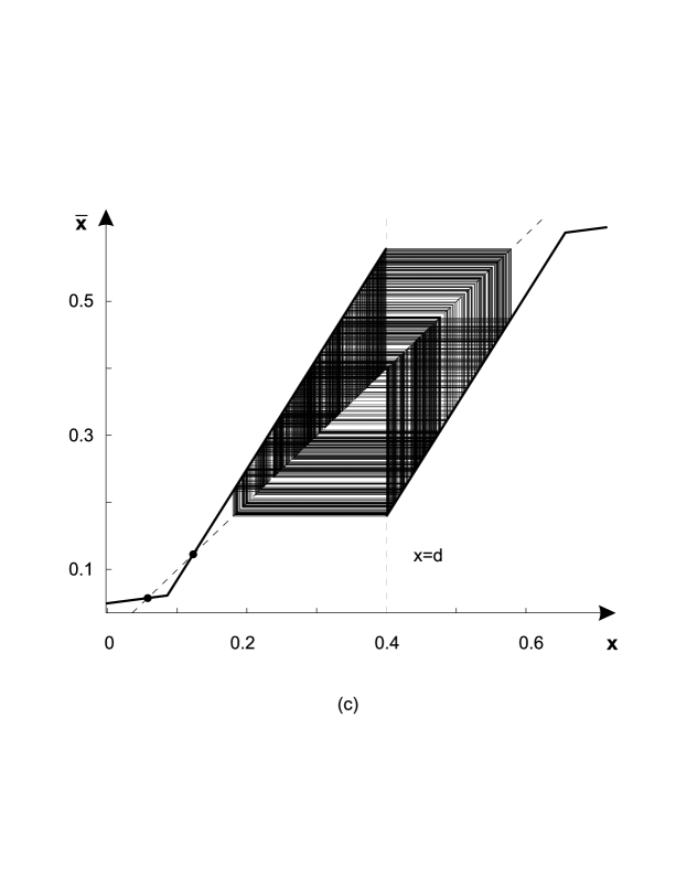
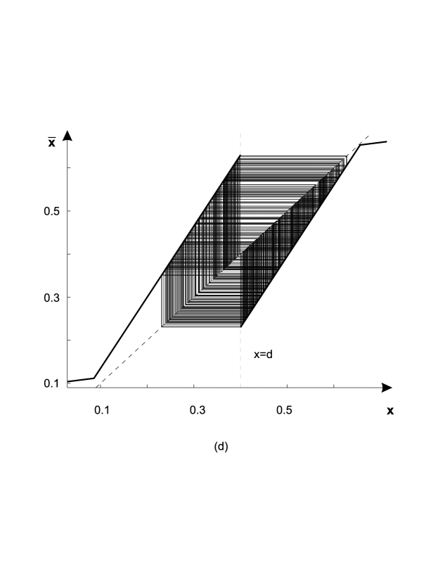
Figure 3: The dynamics of the map $g$ with $m_{0}=0.0864,m_{1}=0.65,a=0.2,d=0.4,\beta=0.4$ for regions: (a) - $Y_{1}$, $y_{0}=0.15$, (b) - $Y_{2}$, $y_{0}=0.05$, (c) - $Y_{4}$, $y_{0}=-0.05$, (d) - $Y_{3}$, $y_{0}=-0.1$.

where $\beta_{0}=F(J_{max})-F(J_{min})$. These conditions allow to obtain interesting properties of the map (3). Let us find the conditions on the parameter values for which the map $f$ acts like a Lorenz-type map b:Afraimovich . For that we require that (see Fig. 3)

$$\lim_{x\nearrow d}g_{2}(x)<g_{3}(J_{max}),\qquad\lim_{x\searrow d}g_{3}(x)>g_{2}(J_{min}).$$ (11)

It follows from (11) the following condition on the parameter $\beta$:

$$\beta<\beta_{1},$$ (12)

where

$$\beta_{1}=min\left\{q(J_{max}-d),q(d-J_{min})\right\}.$$

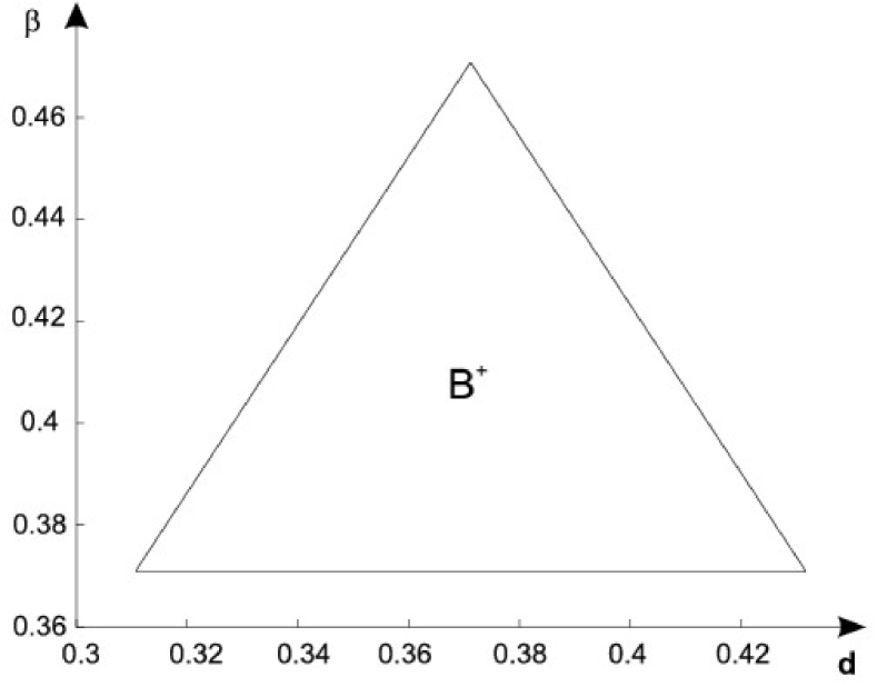
Figure 1: The parameter region $B^{+}$ defined by inequalities (9) and (12) ($m_{0}=0.0864,m_{1}=0.65,a=0.2$)

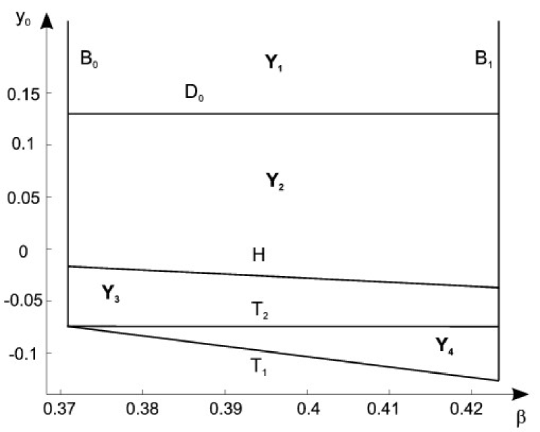
Figure 2: The $Y$ region on the $(\beta,y_{0})$ plane with (9) and (10) ($m_{0}=0.0864,m_{1}=0.65,a=0.2,d=0.4$)

The inequalities (9) and (12) define on the $(d,\beta)$ plane the region $B^{+}$ (see Fig.1). Let us take the parameters $d$ and $\beta$ inside the $B^{+}$ region, and let us consider the $(\beta,y_{0})$ plane. In this plane the inequalities (9), (10) and (12) are satisfied simultaneously in region $Y$. In this plane the boundary of $Y$ consists of the three lines (Fig. 2)

$$B_{0} = \left\{(y_{0},\beta):\beta=\beta_{0},\quad y_{0}\geq F(J_{min})\right\}$$

$$B_{1} = \left\{(y_{0},\beta):\beta=\beta_{1},\quad y_{0}\geq F(J_{max})-\beta_{1}\right\}$$

$$T_{1} = \left\{(y_{0},\beta):y_{0}=F(J_{max})-\beta,\quad\beta_{0}\leq\beta\leq\beta_{1}\right\}.$$

Consider the dynamics of the map $g$ for $(y_{0},\beta)\in Y$. This region is separated on four subregions by the bifurcation lines

$$D_{0} = \left\{(y_{0},\beta):y_{0}=F(d),\quad\beta_{0}\leq\beta\leq\beta_{1}\right\}$$

$$H = \left\{(y_{0},\beta):y_{0}=F(d)-\frac{q-1}{q}\beta,\quad\beta_{0}\leq\beta\leq\beta_{1}\right\}$$

$$T_{2} = \left\{(y_{0},\beta):y_{0}=F(J_{min}),\quad\beta_{0}\leq\beta\leq\beta_{1}\right\},$$

corresponding to different dynamics of the map $g$. The line $D_{0}$ coincides with appearance of an unstable fixed point $x=a+y_{0}/m_{1}$ through crossing of the discontinuity point $x=d$. Line $T_{2}$ corresponds to the fold (tangent) bifurcation of the fixed point $x=J_{min}$ (see Fig. 3(a,d)). Line $H$ corresponds to the condition

$$\lim_{x\searrow d}g_{3}(x)=a+y_{0}/m_{1}.$$

Note that for $(y_{0},\beta)\in H$ there exists a bifurcation corresponding to appearance of homoclinic orbit b:AfraimovichShilnikov to the unstable fixed point. The dynamics of the map $g$ corresponding to subregions $Y_{i}(i=1,..4)$ is shown in Fig.3. If $(\beta,y_{0})\in Y_{1}\bigcup Y_{2}$ the trajectories of the map $g$ tend to stable fixed point $x=-y_{0}/m_{0}$ for any initial conditions different from an unstable fixed point (Fig.3 (a), (b)). If $(\beta,y_{0})\in Y_{3}\bigcup Y_{4}$ the map $f$ has invariant interval $I=\{x:\quad b<x<c\}$, where

$$b = qd-y_{0}-am_{1}-\beta$$ (13)

$$c = qd-y_{0}-am_{1}.$$

For parameters $(\beta,y_{0})\in Y_{3}$ the map $g$ exhibits bistable property, that is there exists two attractors, one is a stable fixed point and the second is an invariant set of the interval $I$ whose basins of attraction are separated by an unstable fixed point (Fig.3(c)). For $(\beta,y_{0})\in Y_{4}$ there exists the interval $I$ (Fig.3 (d)) which attract all trajectories of the map $g$.

Check that the map $g$ on the $I$ acts like a Lorenz-type map. The map $g$ will be a Lorenz-type if b:Afraimovich

1. the derivative $g^{\prime}(x)>0$ for any $x\in I\setminus\{d\}$;

2. the set of preimages of the point of discontinuity, $D=\bigcup\limits_{n\geq 0}g^{-n}(d)$ is dense in $I$;

3. $\lim\limits_{x\searrow d}g(x)=b,\quad\lim\limits_{x\nearrow d}g(x)=c$.

One can see that (i) and (iii) are satisfied. According to b:Afraimovich the condition (ii) is satisfied if

$$g^{\prime}(x)\geq q>1,\quad x\in I\setminus\{d\}.$$ (14)

For the map $g$ on the interval $I$ we have $q=1+m_{1}$ and inequality (14) is obviously satisfied. Therefore the map $g$ on the interval $I$ acts like a Lorenz-type map. The possible structure of the invariant set of interval $I$ is controlled by value $q$.

Let us find conditions under which the map $g$ is strongly transitive. Recall b:Afraimovich that a Lorenz-type map $g$ is strongly transitive if for any subinterval $I_{0}\subset I\setminus\{d\}$ there is $k\geq 0$ such that

$$\bigcup_{i=0}^{k}f^{i}I_{0}\supset IntI.$$

Under the condition (14) the sufficient condition for strong transitivity on the interval $I$ are ( b:Afraimovich )

$$\min\left\{q^{n_{1}+1},q^{n_{2}+1}\right\}>2$$ (15)

where $n_{1},n_{2}\in\mathbb{Z}_{+}$ are such that they satisfy the following conditions

$$g_{2}(b),\ldots,g_{2}^{n_{1}}(b)\in[b,d),g_{2}^{n_{1}+1}(b)\in(d,c]$$ (16)

$$g_{3}(c),\ldots,g_{3}^{n_{2}}(c)\in(d,c],g_{3}^{n_{2}+1}(c)\in[b,d).$$ (17)

Now let us find condition for the parameter values of the map $g$ under which $n_{1}=n_{2}=1$. Consider the condition (16). Let us take $n_{1}=k$, where $k=1,2,\ldots$. It is clear that (16) holds if the parameter $y_{0}$ satisfies the following conditions

$$\begin{cases}y_{0}\geq F(d)-\beta q^{k}(q-1)/(q^{k+1}-1)\\ y_{0}<F(d)-\beta q^{k+1}(q-1)/(q^{k+2}-1).\end{cases}$$ (18)

Let us require that (18) for $k=1$ is satisfied for

$$(\beta,d)\in B^{+},\quad y_{0}\in Y_{3}\bigcup Y_{4}.$$ (19)

From inequalities (9), (12) and the definitions of the boundaries $T_{1}$ and $H$, it follows that this requirement holds if

$$q\geq\frac{1+\sqrt{5}}{2}.$$ (20)

Similarly, for $n_{2}=k$ we get

$$\begin{cases}y_{0}>F(d)-\beta(q^{k+1}-1)/(q^{k+2}-1)\\ y_{0}\leq F(d)-\beta(q^{k}-1)/(q^{k+1}-1).\end{cases}$$ (21)

By the same argument as indicated above we obtain that for $n_{2}=1$ inequalities (21) hold if the conditions (17) are satisfied. For example, let us fix $q=1,65$, that is $m_{1}=0.65$. In this case the map $g|_{I}$ is strongly transitive and therefore it follows from the theorem 3.1.1. of b:Afraimovich that the periodic points are dense in $I$. We note that all of these periodic points are unstable $(q>1)$ and $I$ is a chaotic attractor. Fig.3 (c),(d) illustrates the dynamics of the map $g$ on the interval $I$ for regions $Y_{3}$ and $Y_{4}$ respectively.

IV Relaxation two-dimensional dynamics of the model and spiking-bursting oscillations

In this section consider the case $\varepsilon<<1$ and $J>J_{min}$. This case corresponds to instability of the unique fixed point $O(x=J,y=F(J)$. Since parameter $\varepsilon$ is sufficiently small, the dynamic of the map $f$ is a relaxation b:Arnold similarly by to the case of ODE (1) . The distinctive characteristic of these systems is two time and velocity scales, so-called ”fast” and ”slow” motions. Basically fast motions are provided by ”frozen” system in which slow variables are regarded as a parameters, and it is assumed that small parameter of the system equals to zero. Slow motions with size of order of the small parameter are given by evolution of ”frozen” variable. In case of the map $f$, $x$ is the fast variable and $y$ is the slow one. Let us study the fast and slow motions in our system.

IV.1 Fast and slow motions

The fast motions of the model (3) is approximately described by the map (7). As indicated above, the dynamics of the map (7) can be both, regular and chaotic according to the parameter value (Fig.3). Consider now under conditions (9), (12) slow motions of the map $f$ on the phase plane $(x,y)$ in the region separated by the following inequalities

$$x<J_{min},\quad y>F(J_{max})-\beta$$ (22)

In the case $\varepsilon<<1$ the motions of the map $f$ have slow features within thin layer $M_{1}^{s}(\varepsilon)$ (thickness is of the order $\varepsilon^{\alpha}$, $0<\alpha<1$) b:Arnold near invariant line

$$W_{1}^{S}(\varepsilon)=\left\{(x,y):y=-k_{0}x-b_{0},\quad x<J_{min}\right\},$$

where

$$k_{0}=\frac{m_{0}}{2}+\sqrt{\frac{m^{2}_{0}}{4}-\varepsilon},\quad b_{0}=\frac{\varepsilon J(1-m_{0}+k_{0})}{k_{0}-\varepsilon}.$$ (23)

Directly from the map $f$ it can be obtained that $W_{1}^{S}(\varepsilon)$ is invariant line not only for $\varepsilon\rightarrow 0$ but for $\varepsilon\leq m_{0}^{2}/4$ also. One can see that the dynamics on the line $W_{1}^{S}(\varepsilon)$ is defined by one-dimensional linear map

$$\overline{x}=(1-m_{0}+k_{0})x+b_{0}.$$ (24)

It is clear that the map (24) has stable fixed point $x=J$. Therefore for $J>J_{min}$ the trajectories on $W_{1}^{S}(\varepsilon)$ with initial conditions $x<J_{min}$ moves to the line $x=J_{min}$. All trajectories from layer $M_{1}^{s}(\varepsilon)$ behave in the same way.

Let us now consider the stability of the slow motions from $M_{1}^{s}(\varepsilon)$ relatively to the fast ones. Since in the case $\varepsilon=0$ each point of the $W^{S}(0)$ is stable fixed point of the fast map (7) then invariant curve $W_{1}^{S}(\varepsilon)$ is stable with respect to the fast motions.

IV.2 Relaxation chaotic dynamics

It is follows from the previous description that when $\varepsilon$ is small enough, the structure of the partition of the phase $(x,y)$-plane into trajectories doesn’t significantly change with respect to case of equations (7), (24). The trajectories of the map $f$ are close to the trajectories of (24) within the layer of the slow motions near $W_{1}^{S}(\varepsilon)$ and to the trajectories of (7) outside these layer. Therefore, the motions of the map $f$ are also formed by the slow-fast trajectories.

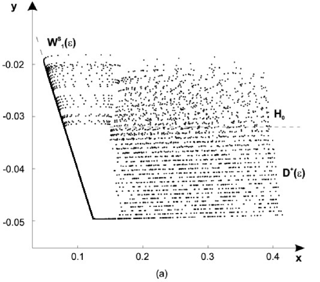
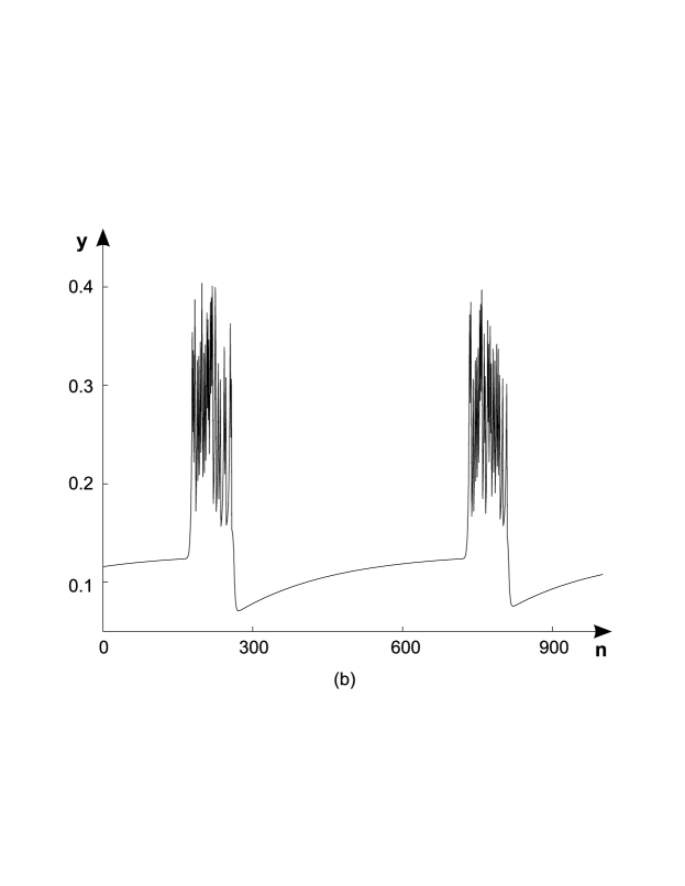
Figure 4: (a) The chaotic attractor $A$ on the phase plane $(x,y)$; (b) Waveform of relaxation spike-bursting oscillations generated by the map $f$. Parameter values: $J=0.13,m_{0}=0.4,m_{1}=0.65,a=0.2,d=0.3,\beta=0.25,\varepsilon=0.002$.

Let the initial conditions of $f$ belong to neighborhood $M_{1}^{S}(\varepsilon)$ of the invariant curve $W_{1}^{S}(\varepsilon)$. Any of these trajectories moves within the layer of the slow motions down to the neighborhood of the critical point $C$ : $x\approx J_{min},y\approx F(J_{min})$, and continue their motions according to the fast motions (see Fig. 3(a)), along $y\approx y_{0}=F(J_{min})$. Since $y_{0}\in Y_{4}$ the trajectory of the map $g$ with initial condition $x\approx J_{min}$ tends to invariant interval $I$ (See Fig. 3 (d)). Therefore the fast motions of the map $f$ with initial conditions $C$ falls into some region $D^{+}(\varepsilon)$ (see Fig 4), $D^{+}(\varepsilon)\rightarrow D^{+}(0)$ if $\varepsilon\rightarrow 0$, where $D(0)$ is the parallelogram:

$$D^{+}(0)=\{(x,y) :$$

$$qd-y-am_{1}-\beta\leq x \leq qd-y-am_{1},$$ (25)

$$F(J_{max})-\beta\leq y \leq F(d)-\beta(q-1)/q\}$$

In other words the region $D^{+}(0)$ is one parametrical family $y_{0}$ - indexed of invariant intervals. As $I$ is attractor, then $D^{+}(\varepsilon)$ is also two-dimensional attracting region. Since the map $g$ has interval $I$ for $y_{0}\in Y_{3}\bigcup Y_{4}$, then a trajectory involving the map $f$ belongs to the region $D^{+}(\varepsilon)$ as long as its variable $y$ do not culminate approximately to the value corresponding to the line $H_{0}$ (Fig. 2). At the same time variable $y$ is slowly increasing for $(x,y)\in D^{+}(\varepsilon)$ as $D^{+}(\varepsilon)\in\{x>J\}$. Thus, within the region $D^{+}(\varepsilon)$ the variable $y$ continues to increase and variable $x$ evolution is close to chaotic trajectory of the map $g$.

Over line $H(y_{0}\in Y_{2})$ the map $g$ has stable fixed point which attracts all trajectories (see Fig.3 (b)). Hence if the magnitude of the variable $y$ becomes about $H$ then trajectory of the map $f$ returns into neighborhood of $M_{1}^{s}(\varepsilon)$. Then the process is repeated. As a result of these slow-fast motions the attractor $A$ of the system $f$ $(x,y)$ phase plane appears as in (Fig.4(a)).

To characterize the complexity of the attractor A we calculated numerically its fractal dimension $d_{f}(A)$. At appears that $d_{f}(A)$ takes non-integer values between 1.35 and 1.9 (Fig.4(b)). Therefore $A$ is chaotic attractor. For the parameter values from Fig. 4 (b) maximum of the fractal dimension $d_{f}(A)=1.8287$ is accomplished then $J=0.2661$.

V Invariant region, chaotic attractor and spiking-bursting oscillations

Let us prove that the system (3) has an attractor $A$ for different values $\varepsilon$ and let us find conditions under which the map $f$ has an invariant region. To do that, we construct some ring-like region $S$. Denote by $\Gamma$ the outer boundary and by $\gamma$ the inner boundary of the $S$. The $S$ is an invariant region if from the conditions $(x,y)\in S$ and $(x,y)\not\in D$ follows that $(\overline{x},\overline{y})\in S$. Its should be fulfilled if

1. the vector field of the map $f$ at the boundary $\Gamma$ and $\gamma$ is oriented inwards to $S$;

2. the images $f_{i}(\Gamma),f_{i}(\gamma),f_{i}(d),i=1,2$ of the boundaries $\Gamma$, $\gamma$ and the discontinuity line $d$ belong to $S$.

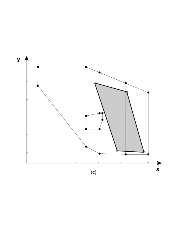
Figure 6: (a) The ring-like invariant region $S$. (b) The image of the region $S\bigcap\{x\leq d\}$ under action of the map $f_{1}$; (c) The image of the region $S\bigcap\{x\geq d\}$ under action of the the map $f_{2}$.

We construct boundaries $\Gamma$ and $\gamma$ in the form of some polygons. Taking into account the condition (i) and analyzing the vector field of the map $f$ at the lines with uncertain slope we have found the shape of $\Gamma$ and $\gamma$ (see Fig. 6 (a)). The equations of the boundaries of $\Gamma$ and $\gamma$ are presented in the Appendix. Analysis of the position of the images $f_{i}(\Gamma),f_{1}(\gamma),f_{i}(d),(i=1,2)$ on the phase plane $(x,y)$ show that the condition (ii) holds if $(\beta,d)\in B^{+}$ (see section III) and inequalities

$$-\frac{\sqrt{\varepsilon}}{m_{0}}(J-J_{min})-m_{0}J-k_{1}(d-J)>F(J_{max})-\beta$$

$$\sqrt{\varepsilon}<\min\left\{\frac{B}{2(d-J)},\frac{m_{0}\left[B-m_{1}(J_{max}-d)\right]}{J-J_{min}}\right\}$$

$$\frac{\sqrt{\varepsilon}}{m_{0}}(J-J_{min})+m_{1}(J_{max}-d)+m_{1}(J_{max}-d)<\frac{B}{2}+\sqrt{\frac{B^{2}}{4}-\varepsilon(d-J)^{2}},\text{ if }\sqrt{\varepsilon}<\frac{B}{2(d-J)}$$

$$\sqrt{\varepsilon}<\frac{\beta-m_{1}(J_{max}-d)}{2(J_{max}-d)},\quad J_{min}<J<\frac{d(1+m_{1})-am_{1}-\beta}{1-m_{0}}$$ (26)

$$\varepsilon(d-J)-\frac{(1+m_{1})(J-J_{min})}{m_{1}}\sqrt{\varepsilon}+(1+m_{1})(d-J)-\beta>0,$$

$$d+F(d)+m_{0}J-J_{max}+\frac{\sqrt{\varepsilon}}{m_{0}}(d-J_{min})+k_{1}(d-J)<0$$

$$\sqrt{\varepsilon}<\min\left\{\frac{m_{0}}{2},\quad\frac{m_{1}}{2},\quad\frac{m_{1}(d-J)}{J-J_{min}}\right\}$$

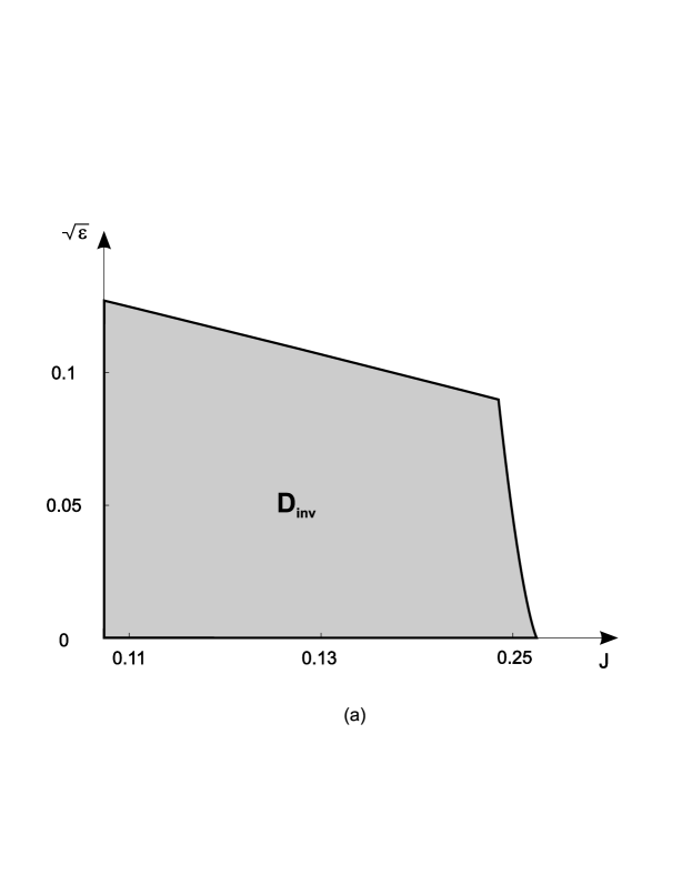
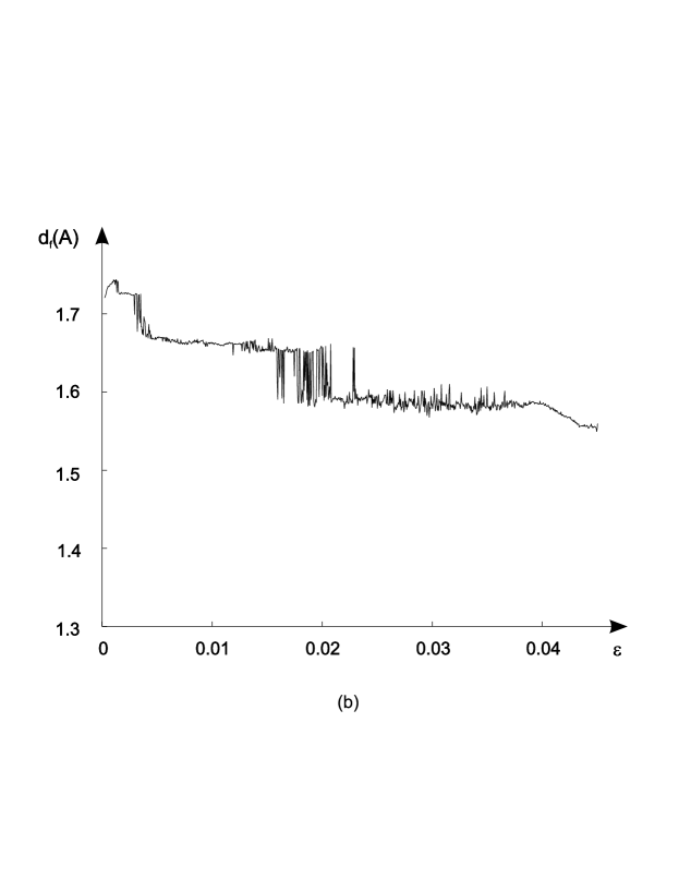
Figure 7: (a) Parameter region $D_{inv}$ on the parameter plane $(J,\varepsilon)$, parameter values: $m_{0}=0.5,m_{1}=0.65,a=0.2,d=0.34,\beta=0.31$. (b) Fractal dimension $d_{f}(A)$ of the attractor $A$ versus parameter $\varepsilon$, $J=0.15$

are satisfied (the parameters $k_{1}$, $B$ and $J_{0}$ have been introduced in Appendix). Fig.6(b),(c) illustrates the transformation of $S$ by the action of the map $f$ under conditions (26). The inequality (26) determine the parameter region $D_{inv}$ in the parameter plane $(J,\varepsilon)$ (Fig. 7 (a)). Since

$$\overline{y}<y,\text{ for }(x,y)\in S\bigcap\{x<J\}$$ (27)

$$\overline{y}>y,\text{ for }(x,y)\in S\bigcap\{x>J\}$$ (28)

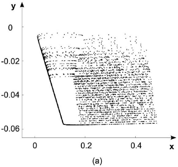
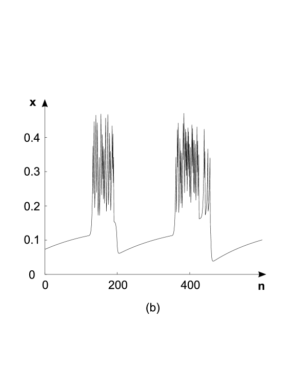
Figure 8: (a) Chaotic attractor $A$ on the phase plane $(x,y)$. (b) Spike-bursting oscillations generated by the map $f$. Parameters value $m_{0}=0.5,m_{1}=0.65,a=0.2,d=0.34,\beta=0.31,J=0.15,\varepsilon=0.004$

then the trajectories with initial conditions $(x,y)\in S$ execute rotation motion around the fixed point $O$ forming some attractors $A$. We calculated numerically fractal dimensional $d_{f}(A)$ (Fig.7(b)) in terms of $\varepsilon$. Its shows that $A$ is chaotic attractor. The possible structure of the attractor $A$ in the phase plane is shown in Fig.8(a). Fig. 8(b) illustrates time evolution of the variable $x$ corresponding to chaotic attractor $A$. It shows chaotic spiking-bursting neural activity. Fig. 7 (b) shows that fractal dimension $d_{f}(A)$, on average, tends to decrease with increasing $\varepsilon$. There is a critical value, $\varepsilon=0.0461$, for which fractal dimension has a minimal value $d_{f}(A)=1.5114$. The mechanism of this decreasing can be accounted for by the different types of the dynamics of the variable $y$ for different $\varepsilon$. As the parameter $\varepsilon$ increases, the velocity of the variable $y$ is expected to climb. Therefore ”life time” of the trajectories in the strip corresponding to Lorenz-map dynamics is reduced. As a result, the chaotical motions are reduced.

VI The gallery of the other attractors and the regimes of neural activity

At previous sections it was shown that system (3) allows to simulate spiking-bursting behavior of the neuron. Here we show that other regimes of the neural activity (phasic spiking and burstings threshold excitation, subthreshold oscillation, tonic spiking and chaotic spike generation) can be obtained by using the map $f$ also. To do that we neglect the first inequality in (6), inequality (9) and condition $y>F(J_{max})-\beta$.

VI.1 The generation of phasic spikes and bursting

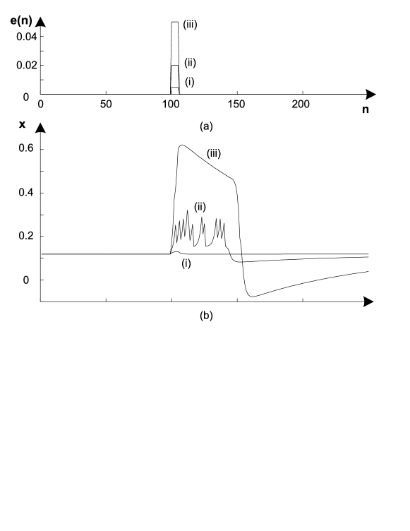
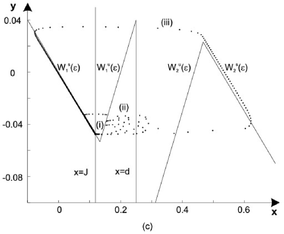
Figure 9: Response of the model (3) to positive pulse $e(n)$: (a) - three different amplitude of the stimulus; (b) - the behavior of variable $x$ (membrane potential of neuron); (c) - the phase plane. Parameter values: $J=0.119,\varepsilon=0.004,d=0.25,\beta=0.19,m_{0}=0.4,m_{1}=0.8,a=0.2$

Studying response of the neurons to the influence of external stimulus is one of important task of neuroscience b:Kandel associated with the problem of information transmission in neural system. Usually external stimulus is represented as the injection of electrical current into the neuron. Let us suppose that the neuron is not excited initially, that is, it is in steady state (rest). In the model (3) such state of neuron corresponds to stable fixed point $O$. Consider the response of the system (3) to pulse type stimulus. We assume that the duration of each pulse is small enough (see Fig. 9(a)) and its action is equal to the instantaneous changing of the variable $x$ on the pulse amplitude. Besides, we suppose here that $\varepsilon<<1$ and therefore the dynamics of the system (3) is a relaxation. For this parameter region the system (3) has two thresholds. The first threshold is determined (see Fig. 9(c)) by the thin layer of the slow motions near the following invariant line

$$W_{1}^{u}(\varepsilon)=\left\{(x,y):y=k_{1}x-b_{1},\quad J_{min}<x<d\right\}$$

where

$$b_{1}=m_{1}a-\frac{\varepsilon J}{k_{1}},\quad k_{1}=\frac{m_{1}}{2}+\sqrt{\frac{m_{1}^{2}}{4}-\varepsilon}.$$

Analogously, the second threshold is defined (see Fig. 9(c)) as the thin layer of the slow motions near invariant line

$$W_{2}^{u}(\varepsilon)=\left\{(x,y):y=k_{1}x-b_{2},\quad d<x<J_{max}\right\},$$

where

$$b_{2}=m_{1}a-\frac{\varepsilon J}{k_{1}}+\beta.$$

Denote by the $x^{e}$ and $y^{e}$ ($y^{e}\approx F(J)$) the values of the variables $x$ and $y$ after stimulation respectively. Let $E$ be the trajectory of the system (3) with this initial conditions. In other words $E$ is response of the system (3) to pulse input.

(i) If the amplitude of stimulus is not enough (Fig. 9(a),(i)) for overcoming the first threshold, then the maximum of the response will be about amplitude of the stimulus. Therefore, in this case the generation of the actions potential does not take place.

(ii) Let us increase the amplitude of the stimulus as it breaks the first threshold but at the same time it is not enough for overcoming of the second threshold (Fig. 9(c),(ii)). In this case the fast motions of the map $f$ will be close to the fast motions of the nap $g$ on interval $I$ for $y_{0}\in Y_{3}\bigcup Y_{4}$. And so, the trajectory of the map $f$ perform some number of irregular oscillations around discontinuity line $x=d$ (Fig. 9(c)(ii)). After that, the trajectory $E$ within layer near $W_{1}^{s}(\varepsilon)$ tends to fixed point $O$ (Fig. 9(c)(ii)). Such trajectory $E$ forms the region of phasic bursting activity b:Izhikevich with irregular number of spikes (Fig. 9(b),(ii)).

(iii) If the amplitude of the stimulus (Fig. 9(a),(iii)) is enough for overcoming the second threshold, then the point $x=x^{e},y=y^{e}$ belongs to the region of attractor of the invariant line $W_{2}^{s}(\varepsilon)$, where

$$W_{2}^{s}(\varepsilon)=\left\{(x,y):y=-k_{0}x-b_{3},\quad x>J_{max}\right\}$$

with

$$b_{3}=-m_{0}a-\frac{\varepsilon J}{k_{0}}+\beta.$$

Therefore trajectory $E$ tends to thin layer of slow motions near invariant line $W_{2}^{s}(\varepsilon)$. It moves within thin layer to the neighborhood of the point $(x\approx J_{max},y=F(J_{max})-\beta)$ (Fig. 9(c),(iii)) and its motions continue along fast motions. These motions are close to the trajectories of the map $g$ for $y_{0}\in Y_{1}$ (see Fig. 3(a)). Therefore the trajectory $E$ tends to the layer near stable invariant line $W_{1}^{s}(\varepsilon)$. After that the trajectory $E$ moves within thin layer near $W_{2}^{S}(\varepsilon)$ and it tends to the fixed point $O$ (Fig. 9(c),(iii)). In this case trajectory $E$ corresponds to phasic spike b:Izhikevich (Fig. 9(b),(iii)).

VI.2 Oscillatory modes of the neural activity

VI.2.1 Close invariant curve and subthreshold oscillations

Let us consider dynamics of the map $f$ under following conditions on the parameters.

$$\varepsilon<m_{0},\quad m_{0}>m_{1}^{2}/4$$

$$\varepsilon>\max\left\{\frac{m_{0}^{2}}{4},\frac{m_{1}^{2}}{4}\right\}.$$

One can see from the Jacobian matrix that in this case the fixed point $O$ has a complex-conjugate multipliers. This point is stable for $J<J_{min}$ and unstable for $J>J_{min}$. Therefore the piece-wise map $f$ produces Neimark-Sacker like bifurcation (in classical case of Neimark-Sacker bifurcation the map is smooth). The fixed point $O$ is surrounded for $J>J_{min}$ by an isolated stable attracting close curve $C_{th}$ (Fig. 10(a)). The oscillations corresponding to the $C_{th}$ occur under the threshold of excitability of the neuron and therefore it is called in neuroscience b:Llinas ; b:LlinasVortex , subthreshold oscillations (Fig. 10(b)).

VI.2.2 ”Two-channel” chaotic attractor and chaotic spiking oscillations

Let us consider again the relaxation ($\varepsilon<<1$) dynamics of the map $f$ in the case $J>J_{min}$, that is when fixed point $O$ is unstable. Additionally we assume that the parameters of the map $f$ has satisfied the following conditions

$$F(J_{min})>F(d)-\beta,$$ (29)

$$F(J_{max})>F(d).$$ (30)

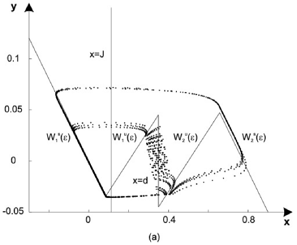
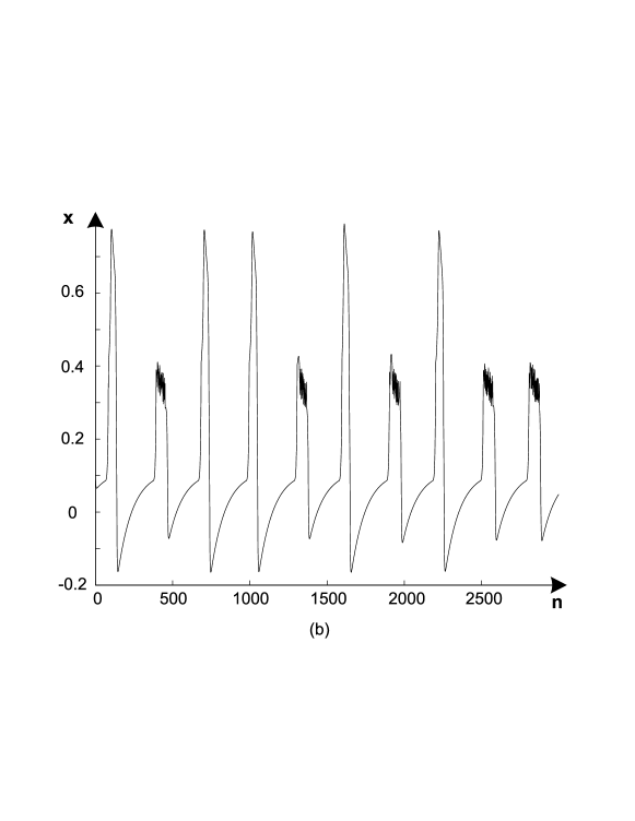
Figure 11: (a) ”Two-channels” chaotic attractor $A_{th}$. (b) Chaotic spiking against the background subthreshold oscillations. Parameter values: $J=0.1123,\varepsilon=0.004,d=0.3,m_{0}=0.4,m_{1}=0.3,a=0.2,\beta=0.09$

In this case the invariant line $W_{2}^{u}(\varepsilon)$ separate the fast motions on two flows (Fig. 11(a)) in the neighborhood of the discontinuity line $x=d$. The first flow forms the trajectory performing the chaotic oscillations near the line $x=d$ (Fig. 11(a)). Their dynamics are close to the dynamics of the map $g$ on interval $I$ for $y_{0}\in Y_{3}\bigcup Y_{4}$. The second flow consists of the trajectories overcoming the second threshold (Fig. 11(a)). It moves to neighborhood of the stable invariant line $W_{2}^{s}(\varepsilon)$. After that these trajectory tends to the stable invariant line $W_{1}^{s}(\varepsilon)$ and the described process is repeated. These trajectories form chaotically switching flow from one to other. As a result is the appearance of a chaotic attractor $A_{th}$ on phase plane (Fig. 11(a)). The fractal dimension $d_{f}(A_{th})=1.30335$. The attractor $A_{th}$ determines chaotic regime of spiking activity over the background of the subthreshold oscillations (Fig. 11(b)).

VI.2.3 Close invariant curve and tonic spiking

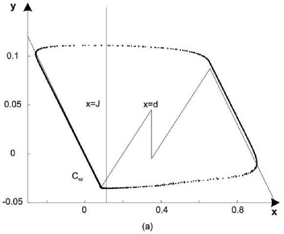
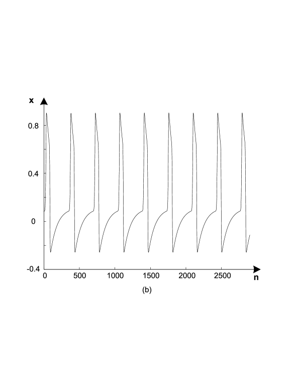
Figure 12: (a) Close invariant curve. (b) Tonic spiking. Parameter values: $J=0.1123,\varepsilon=0.004d=0.3,m_{0}=0.4,m_{1}=0.3,a=0.2,\beta=0.05$

Let the parameters of the map $f$ satisfy the same conditions as in the case of previous subsection VI.2.1 with exception of inequality (29). In this case the parameter $\beta$ is small enough. Therefore the trajectories with initial conditions from neighborhood of $W_{1,2}^{s}(\varepsilon)$ do not change direction of motion when they intersect the discontinuity line $x=d$. This leads to the appearance on the phase plane of the motions between layer near $W_{1}^{s}(\varepsilon)$ and $W_{2}^{s}(\varepsilon)$. Such dynamics leads to forming close invariant curve $C_{sp}$ (Fig. 12(a)). So there exists only one attractor on the phase plane formed by this invariant closed curve. This determines tonic spiking regimes of neural activity (Fig. 12(b)).

VII Conclusion

A new phenomenological model of neural activity is proposed. The model can reproduce basic activity modes such as spiking, chaotic spiking-bursting, subthreshold oscillations etc. of real biological neurons. The model is a discontinous two-dimensional map based on the discrete version of the FitzHugh - Nagumo system and dynamical properties the Lorenz-like map. We have shown that the dynamics of our model display both regular and chaotic behavior. We have studied the underlying mechanism of the generation of chaotic spiking-bursting oscillations. Sufficient condition for existence chaotic attractors in the phase plane are obtained. In spite of idealization, the dynamical modes which are demonstrated in our model are in agreement with the neural activity regimes experimentally found in real biological systems. For example, subthreshold oscillations (see Fig. 10(b)) is a basic regime of inferior olive (I.O.) neurons b:Llinas . Inferior olive neurons belong to the olivo-cerebellar network which plays a key role b:LlinasVortex in organization of vertebrate motor control. It is also typical for I.O. neuron b:Bernardo a spiking regime over the chaotic subthreshold oscillations (see Fig. 11). The spiking-bursting activity is significant for many types of neurons, in particular in hippocampal pyramidal cell b:Wang and thalamic cells b:Deschenes .

The table summarizes results on gallery of behavior of neural activity showed by our model. We hope that our model will be useful to understand the mechanism of neural pattern formation in large networks.

TABLE
Parameters	The regimes of neuronal activity
$J<J_{min}$, $\varepsilon<<1$ $F(J)<F(J_{max})-\beta$, $F(J_{max})-\beta>F(d)$ (spike) $F(J)>F(d)-\beta$ (bursts)	Phasic spikes and bursts
$J>J_{min}$, $\varepsilon<m_{0}$ $m_{0}>m_{1}^{2}/4$ $\varepsilon>\max\left\{\frac{m_{0}^{2}}{4},\frac{m_{1}^{2}}{4}\right\}$	Subthreshold oscillations
Inequalities (26).	Chaotic bursting oscillations
$J>J_{min}$, $\varepsilon<<1$ $F(J_{min})>F(d)-\beta$ $F(J_{max})>F(d)$	Chaotic spiking
$J>J_{min}$, $\varepsilon<<1$ $F(J_{min})<F(d)-\beta$.	Tonic spiking

Appendix. The equations of the boundaries of the invariant region

The boundary $\Gamma$ is given by

$$\Gamma_{1}= \left\{(x,y):d\leq x\leq J_{max},\quad y=-\frac{\sqrt{\varepsilon}}{m_{0}}(J-J_{min})-m_{0}J-k_{1}(d-J)\right\}$$

$$\Gamma_{2}= \left\{(x,y):J\leq x\leq d,\quad y=-p(x-J)-\frac{\sqrt{\varepsilon}}{m_{0}}(J-J_{min})-m_{0}J\right\}$$

$$\Gamma_{3}= \left\{(x,y):J_{min}\leq x\leq J,\quad y=-\frac{\sqrt{\varepsilon}}{m_{0}}(x-J_{min})-m_{0}J\right\}$$

$$\Gamma_{4}= \left\{(x,y):-J_{1}\leq x\leq J_{min},\quad y=-k_{0}(x-J_{min})-m_{0}J\right\}$$

$$\Gamma_{5}= \left\{(x,y):-J_{1}\leq x\leq-J_{0},\quad\sqrt{\varepsilon}y=(x+J_{0})+\sqrt{\varepsilon}m_{0}J_{0}\right\}$$

$$\Gamma_{6}= \left\{(x,y):-J_{0}\leq x\leq J_{min},\quad y=m_{0}J_{0}\right\}$$

$$\Gamma_{7}= \left\{(x,y):J_{min}\leq x\leq J,\quad y=-2\sqrt{\varepsilon}(x-d)+F(d)+\sqrt{\varepsilon}(d-J)\right\}$$

$$\Gamma_{8}= \left\{(x,y):x=J_{max},y_{1}\leq y\leq y_{2}\right\}$$

with

$$y_{1} = -\frac{\sqrt{\varepsilon}}{m_{0}}(J-J_{min})-m_{0}J-k_{1}(d-J)$$

$$y_{2} = -2\sqrt{\varepsilon}(J_{max}-d)+F(d)+\sqrt{\varepsilon}(d-J)$$

$$p=\begin{cases}\frac{B}{2(d-J)}-\sqrt{\frac{B^{2}}{4(d-J)^{2}}-\varepsilon},\quad&\text{if}\quad\sqrt{\varepsilon}\leq\frac{B}{2(d-J)}\\ \frac{B-m_{1}(J_{max}-d)}{d-J},\quad&\text{if}\quad\sqrt{\varepsilon}>\frac{B}{2(d-J)}\end{cases},$$

$$B=\beta-F(d)-m_{0}J,$$

$$J_{0}=\frac{\sqrt{\varepsilon}\left[(d-J)+2(d-J_{min})\right]+F(d)}{m_{0}},$$

$$J_{1}=\frac{(1+\sqrt{\varepsilon}m_{0})J_{0}-\sqrt{\varepsilon}(k_{0}J_{min}-m_{0}J)}{1+k_{0}\sqrt{\varepsilon}}$$

The boundary $\gamma$ is given by

$$\gamma_{1}= \left\{(x,y):J_{min}\leq x\leq J,\quad y=-m_{0}J_{min}\right\}$$

$$\gamma_{2}= \left\{(x,y):x=J_{min},\quad-m_{0}J_{min}\leq y\leq m_{1}(J-a)\right\}$$

$$\gamma_{3}= \left\{(x,y):J_{min}\leq x\leq J,\quad y=m_{1}(J-a)+\sqrt{\varepsilon}(x-J_{min})\right\}$$

$$\gamma_{4}= \left\{(x,y):J\leq x\leq J+\frac{\sqrt{\varepsilon}(J-J_{min})}{m_{1}},\quad y=m_{1}(J-a)+\sqrt{\varepsilon}(J-J_{min})\right\}$$

$$\gamma_{5}= \left\{(x,y):x=J+\frac{\sqrt{\varepsilon}(J-J_{min})}{m_{1}},\quad y_{3}\leq y\leq y_{4}\right\}$$

$$\gamma_{6}= \left\{(x,y):J\leq x\leq J+\frac{\sqrt{\varepsilon}(J-J_{min})}{m_{1}},\quad y=\sqrt{\varepsilon}(x-J)-m_{0}J_{min}\right\}$$

with

$$y_{3} = \frac{\varepsilon(J-J_{min})}{m_{1}}-m_{0}J_{min}$$

$$y_{4} = m_{1}(J-a)+\sqrt{\varepsilon}(J-J_{min})$$

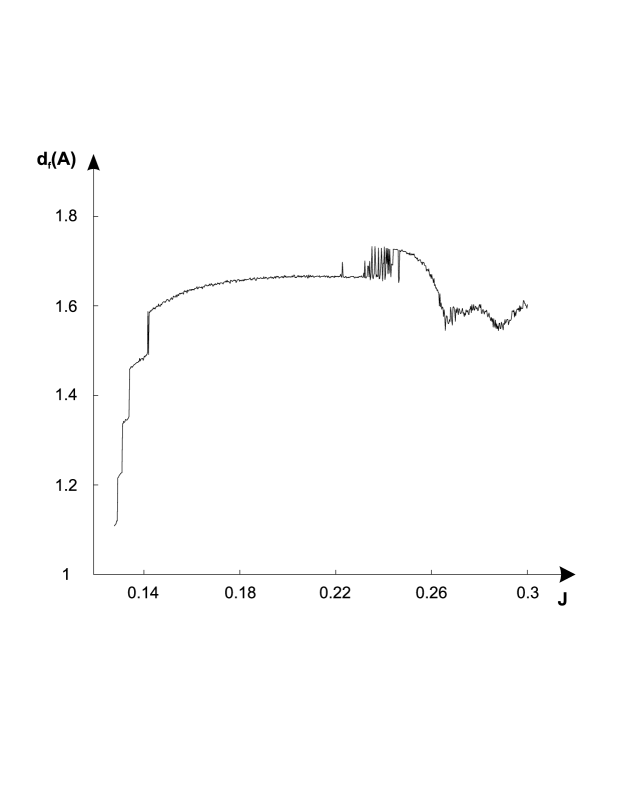
Figure 5: Fractal dimension $d_{f}(A)$ of the attractor $A$ versus parameter $J$. Parameter values: $m_{0}=0.4,m_{1}=0.65,a=0.2,d=0.3,\beta=0.25,\varepsilon=0.002$

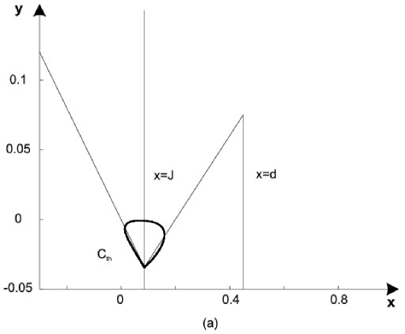
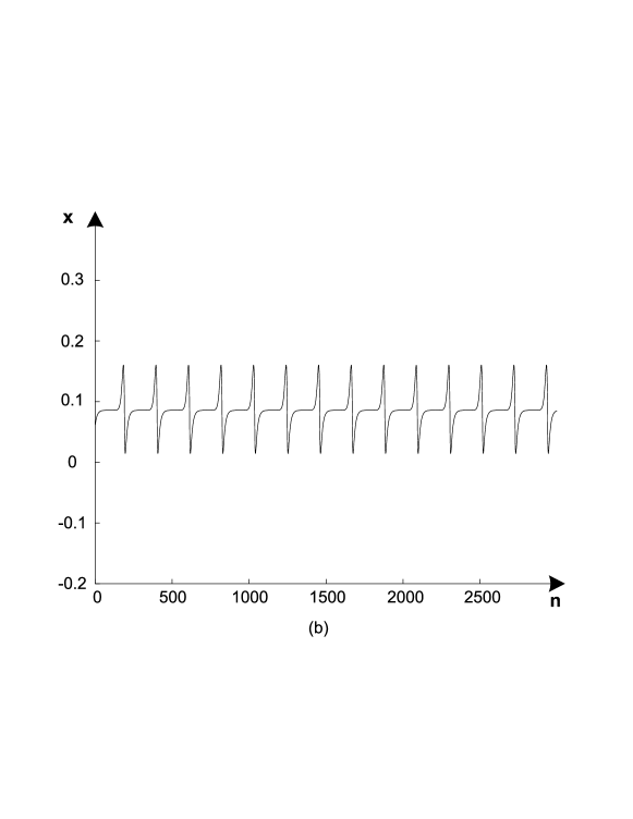
Figure 10: (a) Close invariant curves on the phase plane $(x,y)$. (b) Subthreshold oscillations generated by map $f$. Parameter values: $d=0.3,m_{0}=0.4,m_{1}=0.3,a=0.2,J=0.08572,\varepsilon=0.025,\beta=0.3$

References

- (1) E.R. Kandel, J.H. Schwartz, T.M Jessell, Principles of neural science, Prentice-Hall Int. Inc., 1991.
- (2) M.I. Rabinovich, P. Varona, A.I. Selverston, H.D.I. Abarbanel, Dynamical principles in neuroscience, Reviews of Modern Physics, 78(4) (2006), 1213.
- (3) H.R. Wilson, J.D.Cowan Excitatory and inhibitory interaction in localized population of model neurons. Biophys. J., 12 (1972), pp 1-24.
- (4) R. FitzHugh Mathematical models of the threshold phenomena in the nerve membrane. Bull Math. Biohys. v.17, pp. 257-287 (1955)
- (5) J.L. Hindmarsh , R.M. Rose , A model of neuronal bursting using three coupled first order differential equations: Philos. Trans R. Soc. London, Ser. B221, 87-102 (1984).
- (6) C. Morris, H. Lecar, Voltage oscillations in the barnacle giant muscle fiber. Biophys. J. v25, 1981, p. 87
- (7) D.R. Chialvo, Generic excitable dynamics on the two-dimensional map, Chaos Solitons Fract. 5 (1995) 461-480.
- (8) O. Kinouchi, M. Tragtenberg, Modeling neurons by simple maps, Int. J. Bifurcaton Chaos 6, N 12 a (1996), 2343-2360.
- (9) S.Kuva, G.Lima, O.Kinouchi, M.Tragtenberg, A. Roque, A mimimal model for excitable and bursting element. Neurocomputing 38-40, pp. 255-261 (2001).
- (10) G. de Vries, Bursting as an emergent phenomenon in coupled chaotic maps, Phys. Rev. E 64 (2001) 051914.
- (11) N.F. Rulkov, I.Timofeev, M. Bazhenov, Oscillations in large-scale cortical networks: map-based model. J. of Computational Neuroscince 17 (2004), 203-223.
- (12) R.D. Traub, J.G.R. Jefferys, M.A. Whittington, Fast Oscillations in Cortical Circuits. The MIT Press, Massachusettes, 1999.
- (13) Llinas R. and Yarom, Y., Oscillatory properties of guinea-pig inferioir olivary neurines and their pharmacological modulation: An in vitro study. J. Physol., Lond., 315, 569-84, 1986.
- (14) Llinas R., I of vortex. From Neurones to Self.The MIT Press, Massachusettes, 2002.
- (15) B. Cazelles, M. Courbage, M. Rabinovich, Anti-phase regularization of coupled chaotic maps modelling bursting neurons. Europhysics Letters, 56 (4), pp. 504-509 (2001).
- (16) N.F. Rulkov, Regularization of synchronized chaotic bursts, Phys. Rev. Lett. 86, 183-186 (2001)
- (17) N.F. Rulkov. Modeling of spiking-bursting neural behavior using two-dimensional map. Phys. Rev.E, v.65, p. 0.41922 (2002).
- (18) A.L. Shilnikov, N.F. Rulkov. Origin of chaos in a two dimensional map modeling spiking-bursting neural activity. Int. J. Bifurc. Chaos, v.13, N11, pp. 3325-3340 (2003).
- (19) A.L. Shilnikov, N.F. Rulkov. Subthreshold oscillations in a map-based neron model. Physics Letters A 328, pp. 177-184 (2004).
- (20) H. Tanaka Design of bursting in two-dimensional discrete-time neron model.Physics Letters A 350, pp. 228-231 (2006).
- (21) M.Courbage, V.B. Kazantsev, V.I. Nekorkin, V. Senneret. Emergence of chaotic attractor and anti-synchronization for two coupled monostable neurons. Chaos 12, pp. 1148-1156 (2004).
- (22) E.M. Izhikevich, F. Hoppensteadt, Classification of bursting mappings. Int. J. Bifurcation and Chaos, v.14, N11, pp 3847-3854, (2004).
- (23) V.S. Afraimovich, Sze-Bi Hsu. Lectures on Chaotic Dynamical Systems, American Mathematical Society. Int. Press, 354 p. (2003)
- (24) V.S. Afraimovich, L.P. Shilnikov. Strange attractors and quasiattractors. In book ”Nonlinear Dynamics and Turbulence” (eds. G.I. Barenblatt, G. Iooss, D.D. Joseph, Pitam, Boston, 1983, pp. 1-34
- (25) V.I. Arnold, V.S. Afraimovich, Yu. S. Ilyashenko,L.P. Shilnikov. Bifurcation Theory,Dyn. Sys. V. Encyclopaedia Mathematics Sciences, Springer, Berlin, 1994
- (26) Bernardo L.S., Foster R.P. Oscillatory behaviour in the inferior olive neurons : mechanism, modulation, cell agregates. Brain Res. Bull. 1986, v.17, p.773
- (27) R.S.K. Wang and D.A. Prince Afterpotential generation in hippocampal pyramidal cells. J. Neurophysiol. v45, 1981, p.86
- (28) M. Deschenes, J.P. Roy and M. Steriade Thalamic bursting mechanism: an inward slow current revealed by membrane hyperpolarization. Brain Res. 239, 1982, p.289.