Hinged Dissections Exist

Abstract

We prove that any finite collection of polygons of equal area has a common hinged dissection. That is, for any such collection of polygons there exists a chain of polygons hinged at vertices that can be folded in the plane continuously without self-intersection to form any polygon in the collection. This result settles the open problem about the existence of hinged dissections between pairs of polygons that goes back implicitly to 1864 and has been studied extensively in the past ten years. Our result generalizes and indeed builds upon the result from 1814 that polygons have common dissections (without hinges). We also extend our common dissection result to edge-hinged dissections of solid 3D polyhedra that have a common (unhinged) dissection, as determined by Dehn’s 1900 solution to Hilbert’s Third Problem. Our proofs are constructive, giving explicit algorithms in all cases. For a constant number of planar polygons, both the number of pieces and running time required by our construction are pseudopolynomial. This bound is the best possible, even for unhinged dissections. Hinged dissections have possible applications to reconfigurable robotics, programmable matter, and nanomanufacturing.

1 Introduction

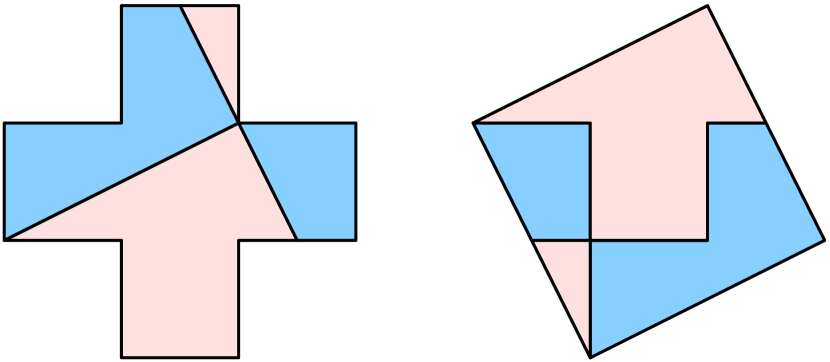
Figure 1: 4-piece dissection of Greek cross to square from 1890 [Lem90].

Around 1808, Wallace asked whether every two polygons of the same area have a common dissection, that is, whether any two equal-area polygons can be cut into a finite set of congruent polygonal pieces [Fre97, p. 222]. Figure 1 shows a simple example. Lowry [Low14] published the first solution to Wallace’s problem in 1814, although Wallace may have also had a solution at the time; he published one in 1831 [Wal31]. Shortly thereafter, Bolyai [Bol33] and Gerwien [Ger33] rediscovered the result, whence this result is sometimes known as the Bolyai-Gerwien Theorem.

By contrast, Dehn [Deh00] proved in 1900 that not all polyhedra of the same volume have a common dissection, solving Hilbert’s Third Problem posed in the same year [Deh00]. Sydler [Syd65] showed that Dehn’s invariant in fact characterizes 3D dissectability.

Lowry’s 2D dissection construction, as described by Frederickson [Fre97], is particularly elegant and uses a pseudopolynomial number of pieces. A pseudopolynomial bound is the best possible in the worst case: dissecting a polygon of diameter $x>1$ into a polygon of diameter $1$ (for example, a long skinny triangle into an equilateral triangle) requires at least $x$ pieces. With this worst-case result in hand, attention has turned to optimal dissections using the fewest pieces possible for the two given polygons. This problem has been studied extensively for centuries in the mathematics literature [Oza78, Coh75, Fre97] and the puzzle literature [Pan49, Lem90, Mad79, Lin72], and more recently in the computational geometry literature [CKU99, KKU00, ANN⁺03].

Hinged dissections are dissections with an additional constraint: the polygonal pieces must be hinged together at vertices into a connected assembly. The first published hinged dissection appeared in 1864, illustrating Euclid’s Proposition I.47 [Kel64]; see [Fre02, pp. 4–5]. The most famous hinged dissection is Dudeney’s 1902 hinged dissection [Dud02]; see Figure 2. This surprising construction inspired many to investigate hinged dissections; see, for example, Frederickson’s book on the topic [Fre02].

However, the fundamental problem of general hinged dissection has remained open [DMO03, O’R02]: do every two polygons of the same area have a common hinged dissection? This problem has been attacked in the computational geometry literature [AN98, DDE⁺05, Epp01, DDLS05], but has only been solved in special cases. For example, all polygons made from edge-to-edge gluings of $n$ identical subpolygons (such as polyominoes) have been shown to have a common hinged dissection [DDE⁺05]. Perhaps most intriguingly, Eppstein [Epp01] showed that the problem of finding a hinged dissection of any two triangles of equal area is just as hard as the general problem.

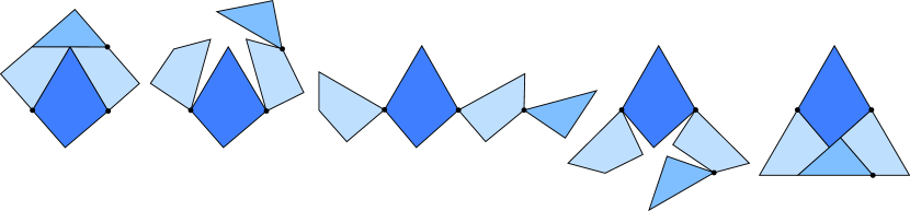
Figure 2: Dudeney’s 1902 hinged dissection of a square into a triangle [Dud02].

Hinged dissections are particularly exciting from the perspectives of reconfigurable robotics, programmable matter, and nanomanufacturing. Recent progress has enabled chemists to build millimeter-scale “self-working” 2D hinged dissections such as Dudeney’s [MTW⁺02]. An analog for 3D hinged dissections may enable the building of a complex 3D structure out of a chain of units; see [Gri04] for one such approach. We could even envision an object that can re-assemble itself into different 3D structures on demand [DDLS05]. This approach contrasts existing approaches to reconfigurable robotics (see, for example, [RBKV02]), where units must reconfigure by attaching and detaching from each other through a complicated mechanism.

Our results.

We settle the hinged dissection open problem, first formally posed in a CCCG 1999 paper [DDE⁺05] but implicit back to 1864 [Kel64] and 1902 [Dud02]. Specifically, Section 3 proves a universality result: any two polygons of the same area have a common hinged dissection. In fact, our result is stronger, building a single hinged dissection that can fold into any finite set of desired polygons of the same area. The analogous multipolygon result for (unhinged) dissections is obvious—simply overlay the pairwise dissections—but no such general combination technique is known for hinged dissections. Indeed, the lack of such a transitivity construction has been the main challenge in constructing general hinged dissections.

Our construction starts from an arbitrary (unhinged) dissection, such as Lowry’s [Low14]. We show that any dissection of a finite set of polygons can be subdivided and hinged so that the resulting hinged dissection folds into all of the original polygons. We give a method of subdividing pieces of a hinged figure which effectively allows us to “unhinge” a portion of the figure and “re-attach” it at an alternate location. This construction allows us to “move” pieces and hinges around arbitrarily, at the cost of extra pieces. Therefore, we are able to hinge any dissection.

This naïve construction easily leads to an exponential number of pieces, but we show in Section 5 that a more careful execution of Lowry’s dissection [Low14] attains a pseudopolynomial number of pieces for a constant number of target polygons. As mentioned above, such a bound is essentially best possible, even for unhinged dissections. This more efficient construction requires significantly more complex gadgets for simultaneously moving several groups of pieces at roughly the same cost as moving a single piece, and relies on specific properties of Lowry’s dissection.

We also solve another open problem concerning the precise model of hinged dissections. In perhaps the most natural model of hinged dissections, pieces cannot properly overlap during the folding motion from one configuration to another. However, all theoretical work concerning hinged dissections [AN98, DDE⁺05, Epp01, DDLS05] has only been able to analyze the “wobbly hinged” model [Fre02], where pieces may intersect during the motion. Is there a difference between these two models? Again this problem was first formally posed at CCCG 1999 [DDE⁺05]. We prove in Section 4 that any wobbly hinged dissection can be subdivided to enable continuous motions without piece intersection, at the cost of increasing the combinatorial complexity of the hinged dissection by only a constant factor. This result builds on expansive motions from the Carpenter’s Rule Theorem [CDR03, Str05] combined with the theory of slender adornments from SoCG 2006 [CDD⁺06].

The following theorem summarizes our results for 2D figures:

Theorem 1.

Any finite set of polygons of equal area have a common hinged dissection which can fold continuously without intersection between the polygons. For a constant number of target polygons with vertices drawn on a rational grid, the number of pieces is pseudopolynomial, as is the algorithm to compute the common hinged dissection.

Finally, we generalize our results to 3D in Section 6. As mentioned above, not all 3D polyhedra have a common dissection even without hinges. Our techniques generalize to show that hinged dissections exist whenever dissections do:

Theorem 2.

If two 3D polyhedra have the same volume and Dehn invariant, then they have a common hinged dissection.

2 Terminology

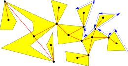
Figure 3: A hinged figure, its incidence graph (red), and part of is boundary path.

A hinged figure $F$ is a finite collection of simple, oriented polygons (the links) hinged together at rotatable joints at the links’ vertices so that the resulting figure is connected, together with a fixed cyclic order of links around each hinge. (Note that a hinge might exist at a $180^{\circ}$ angle of a link, but this hinge is still considered a vertex of the link.) A configuration of a hinged figure $F$ is an embedding of $F$’s links into the plane so that the links’ interiors are disjoint and so that each hinge’s cyclic link order is maintained.

The incidence graph of a hinged figure is the graph that has a vertex corresponding to every link and every hinge, such that two nodes are connected by an edge if one represents a link and the other represents a hinge on that link. See Figure 3. A hinged figure is tree-like if the incidence graph is a tree, and it is chain-like if the incidence graph is an open chain.

The boundary $\partial A$ of a hinged figure $A$ is the oriented path (or collection of paths) along the edges of the links traversed in depth-first order, as illustrated in Figure 3. For a tree- or chain-like figure, the boundary consists of a single path incorporating all edges of the links. Note that the boundary path will trace each hinge point multiple times, but we distinguish these as different boundary points.

For two hinged figures $A$ and $B$, we say that $B$ is a refinement of $A$, and write $B\prec A$, if $A$ can be obtained from $B$ by gluing together portions of $B$’s boundary, i.e., by adding hinges between pieces of $B$ which may effectively glue together shared edges of pieces in $B$. Intuitively, one could obtain $B$ from $A$ by cutting the pieces in $A$ and breaking some of the hinges. The gluing in the definition gives rise to an imposed configuration of $B$ for every configuration of $A$. The property of refinement is transitive; that is, if $C\prec B$ and $B\prec A$, then $C\prec A$. This transitivity of refinement plays a central role in the arguments below.

3 Universal Hinged Dissection

In this section, we show that any finite collection of equal-area polygons has a common hinged dissection. More precisely, we construct a hinged figure with a configuration in the shape of every desired polygon; continuous motions without intersection will be addressed in Section 4. The proof is in three parts: effectively moving rooted subtrees, effectively moving rooted pseudosubtrees, and arbitrarily rearranging pseudotrees.

3.1 Moving Rooted Subtrees

Consider a tree-like hinged figure $F$. If there are two hinged figures $A$ and $B$ with two distinguished boundary points $a\in\partial A$ and $b\in\partial B$ so that $F$ is equivalent to the hinged figure obtained by identifying points $a$ and $b$ to a single hinge (denoted $F={A}_{(a)}\wedge{}_{(b)}{B}$), then we say $A$ and $B$ are each rooted subtrees of $F$. If another boundary point $b^{\prime}\in\partial B$ is chosen, then the new hinged figure $F^{\prime}={A}_{(a)}\wedge{}_{(b^{\prime})}{B}$ is related to $F$ by a rooted subtree movement: $(A,a)$ is the subtree that has been moved.

Our goal is to accomplish this movement with hinged dissection. We will achieve this goal by connecting pieces with chains of isosceles triangles hinged at their base vertices. We begin with a lemma concerning cutting isosceles triangles from polygons, and then proceed to construct the required dissection by cutting out chains from both $A$ (at the point $a$) and $B$ (along the boundary from $b$ to $b^{\prime}$).

For an angle $\alpha<90^{\circ}$ and a length $\ell$, denote by $\mathcal{T}_{\alpha}(\ell)$ the isosceles triangle with base of length $\ell$ and base-angles $\alpha$. For a segment $PQ$, use the notation $\mathcal{T}_{\alpha}(PQ)$ for the triangle $\mathcal{T}_{\alpha}(|PQ|)$ drawn with base along segment $PQ$. Finally, for an angle $\beta$, point $P$, and radius $r$, let $\mathcal{S}_{\beta}(P,r)$ be a circular sector centered at $P$ with angle $\beta$ and radius $r$.

Lemma 3.

For any simple polygon $V=V_{1}\ldots V_{n}$, there exist an angle $\beta$ and a radius $r$ small enough so that the triangles $\mathcal{T}_{\beta}(V_{i}V_{i+1})$ constructed inward along the edges, as well as circular sectors $\mathcal{S}_{\beta}(V_{i},r)$ drawn inside $V$, are pairwise disjoint except at the vertices of $V$. These triangles and sectors will be called the free-regions for their respective edges or vertices of $V$.

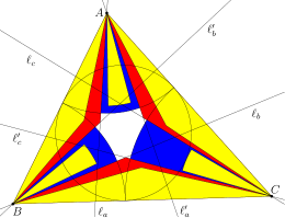
Figure 4: The free regions (lightly colored) in triangle $ABC$ are separated by the dark circles and the angle trisectors $\ell_{a}$, $\ell_{a}^{\prime}$, etc.

Proof.

We first prove the result for triangles. For triangle $T=ABC$ with side lengths $a,b,c$, semiperimeter $s=\frac{1}{2}(a+b+c)$, and angles $\delta,\epsilon,\zeta$, choose $\beta_{T}<\frac{1}{3}\min\{\delta,\epsilon,\zeta\}$ and $r_{T}<\min\{s-a,s-b,s-c\}$. Then the triangles $\mathcal{T}_{\beta_{T}}(AB)$, etc., and the sectors $\mathcal{S}_{\beta_{T}}(A,r_{T})$, etc., can be drawn in the triangle without overlap, as in Figure 4: Indeed, $\mathcal{T}_{\beta_{T}}(AB)$ is contained between $AB$ and the two trisectors $\ell_{a}$ and $\ell_{b}^{\prime}$ (the region shown in red), sector $\mathcal{S}_{\beta_{T}}(A,r_{T})$ is contained in the sector $\mathcal{S}_{\frac{\delta}{3}}(A,s-a)$ between trisectors $\ell_{a}$ and $\ell_{a}^{\prime}$ (shown in green), etc., and these six regions are interior-disjoint.

For the general case, first triangulate polygon $V=V_{1}\cdots V_{n}$ by $n-2$ diagonals. For each triangle $T=V_{i}V_{j}V_{k}$ in the triangulation, calculate $\beta_{T}$ and $r_{T}$ as above, and draw the free regions in $T$. Finally, as all resulting triangles and sectors are disjoint (except at vertices), choosing $\beta=\min_{T}\{\beta_{T}\}$ and $r=\min_{T}\{r_{T}\}$ suffices. ∎

For a sequence of positive lengths $\ell_{1},\ldots,\ell_{n}$, we define the chain $\mathcal{C}_{\alpha}(\ell_{1},\ldots,\ell_{n})=C$ to be the hinged figure formed by hinging the $2n$ upward-pointing triangles

$$\mathcal{T}_{\alpha}(\ell_{1}),\mathcal{T}_{\alpha}(\ell_{1}),\mathcal{T}_{\alpha}(\ell_{2}),\mathcal{T}_{\alpha}(\ell_{2}),\ldots,\mathcal{T}_{\alpha}(\ell_{n}),\mathcal{T}_{\alpha}(\ell_{n})$$

in order at their base vertices. The initial point $C_{0}$ and final point $C_{1}$ of this chain are the unhinged vertices of the first $\mathcal{T}_{\alpha}(s_{1})$ and the last $\mathcal{T}_{\alpha}(s_{n})$ respectively.

We may now state and prove the desired result of this section.

Theorem 4.

For any two tree-like figures $F$ and $F^{\prime}$ related by the rooted subtree movement of $(A,a)$ from $(B,b)$ to $(B,b^{\prime})$, there exists a common refinement $G\prec F$ and $G\prec F^{\prime}$. Further, if $a$ lies on link $L_{a}\in A$, and a simple path $\gamma$ along $\partial B$ is chosen from $b$ to $b^{\prime}$, this refinement $G\prec F$ may be chosen so that only $L_{a}$ and links incident with $\gamma$ are refined.

Note first that both $A$ and $B$ are tree-like, as they are subtrees of tree-like figure $F$. Note also that there are exactly two boundary paths $\gamma$ from $b$ to $b^{\prime}$ since $B$ is tree-like.

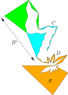
(a)

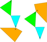
(b)

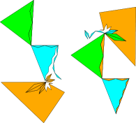
(c)

Figure 5: Effectively moving a rooted subtree

Proof.

Without loss of generality, the diagram is oriented so that $\gamma$ traces the boundary of $B$ counterclockwise from $b$. The construction is in two steps.

In the first step, we cut a chain from the boundary of $\gamma$, as follows. Let $r$ be the smallest free-region radius for all links touched by $\gamma$, and likewise let $\alpha$ be the smallest free-region angle. Path $\gamma$ is a polygonal path $P_{0}P_{1}\ldots P_{t}$ along the boundary of $B$, where $P_{i}$ are vertices of links with $P_{0}=b$ and $P_{t}=b^{\prime}$. By refining this path into shorter segments as necessary, we may assume that each segment $P_{i-1}P_{i}$ has length $2\ell_{i}$ with $\ell_{i}\leq r$.

Choose an angle $\beta<\alpha/2t$. Next, cut out $2t$ isosceles triangles along $\gamma$: for each segment $P_{i}P_{i+1}\in\gamma$, cut two $\mathcal{T}_{\beta}(\ell_{i})$ triangles. These triangles fit in the appropriate free-triangle for their link in $B$ by choice of $\beta$, so all of these triangles may indeed be removed without overlapping or disconnecting any of $B$’s links. Let $B^{*}$ be the hinged figure after these triangles have been removed, and let $C=\mathcal{C}_{\beta}(\ell_{1},\ldots,\ell_{t})$ be the chain formed by hinging these $2t$ cut-out triangles in order. Finally, rehinge the pieces to form the figure $G_{b}={B^{*}}_{(b^{\prime})}\wedge{}_{(C_{1})}{C}$. See Figure 5 for an illustration.

The other step is to cut a chain away from $A$ at $a$. Draw $t$ abutting rhombi $r_{1},\ldots,r_{t}$ in link $L_{a}$ at point $a$ so that $r_{i}$ has a diagonal of length $\ell_{i}$ and an angle of $2\beta$; they are drawn in the order $r_{1},\ldots,r_{k}$ clockwise around $a$ so that $r_{i}$ shares (part of) an edge with $r_{i+1}$ for $1\leq i\leq k-1$. Call this configuration of kites a kite-sweep $\mathcal{KS}_{\beta}(\ell_{1},\ldots,\ell_{n})$. Recall that $\beta$ was chosen so that $2t\beta<\alpha$ and that $\ell_{i}$ were chosen so that $\ell_{i}<r$ for each $1\leq i\leq r$, so this kite-sweep can fit within the free-sector of $L_{a}$ at $a$. Finally, cut out these $t$ rhombi in the form of $2t$ $\beta$-triangles, rehinging them into $D=\mathcal{C}_{\beta}(\ell_{1},\ldots,\ell_{t})$. Link $L_{a}$ is no longer a simple polygon, so simply cut away a small corner near $a$ and rehinge it as shown in Figure 5. Let $A^{*}$ be the remaining hinged figure after $A$ has been thus mutilated. Finally, hinge all of $A$ back together in the form $G_{a}={A^{*}}_{(a)}\wedge{}_{(d_{1})}{D}$.

The final result of our construction is the single hinged figure $G={G_{a}}_{(D_{0})}\wedge{}_{(b)}{G_{b}}$; I claim $G\prec F$ and $G\prec F^{\prime}$. To see $G\prec F$, simply configure chains $C$ and $D$ so that each link assumes the spot from which it was cut from $F$; i.e., chain $C$ fills the triangular holes left along path $\gamma$, and chain $D$ fills the kite-sweep in $L_{a}$. See Figure 5(c), left. For the refinement $G\prec F^{\prime}$, the chains simply switch roles: chain $D$ now fills in the gaps left along $\gamma$, and chain $C$ fills the kite holes in $L_{a}$. See Figure 5(c), right. ∎

3.2 Moving Rooted Pseudosubtrees

Now we increase the level of abstraction by allowing movement of rooted subtrees in a hinged figure $F$ that already has a refinement $G\prec F$. We call $F$ the pseudofigure of $G$, and subtrees of $F$ pseudosubtrees of $G$.

Theorem 5.

Take tree-like figures $F$ and $F^{\prime}$ related by the rooted-subtree movement of $(A,a)$ from $(B,b)$ to $(B,b^{\prime})$ as in Theorem 4, and suppose $G\prec F$. Then there exists a common refinement $H\prec G\prec F$ and $H\prec F^{\prime}$. Further, if a path $\gamma$ from $b$ to $b^{\prime}$ on $\partial B$ is chosen, then only links of $G$ incident with $\gamma$ are refined.

In other words, this theorem allows the movement of a pseudo-subtree of $G$. The construction below directly generalizes the method used in Theorem 4.

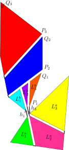
(a)

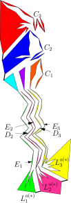
(b)

(c)

Figure 6: Moving a rooted pseudosubtree.

Proof.

We will write from $G$’s point of view, so features of $F$ will have the pseudo prefix. Without loss of generality, suppose $\gamma$ winds counterclockwise around the pseudoboundary of $B$.

Consider the behavior near the pseudohinge $h$ of $F$ corresponding to points $a$ and $b$; let $\{h_{i}\mid 1\leq i\leq n\}$ be the set of all the hinges of $G$ with the property that $h_{i}$ has two incident links $L_{i}^{a}$ and $L_{i}^{b}$ lying in $A$ and $B$ respectively. As links are defined to be simple polygons, these $2n$ links are distinct. We may suppose that these $2n$ links are the only links of $G$ incident with pseudo-hinge $h$: the construction below is unchanged by the presence of more, extraneous links. Without loss of generality, we may assume that these links have been numbered so that they fall in the cyclic order $L_{1}^{a},\ldots,L_{n-1}^{a},L_{n}^{a},L_{n}^{b},L_{n-1}^{b},\ldots,L_{1}^{b}$ counterclockwise around $h$.

Our goal is to mimic the two steps in the proof of Theorem 4, by effectively cutting a chain from $A$ at $a$ and cutting a chain from $B$ along $\gamma$.

We begin by choosing the dimensions of the chain. First, the refinement $G\prec F$ induces an identification of some boundary points of $G$, and any point $p\in\partial G$ collocated with a vertex of any link in $G$ will itself be declared a (possibly flat) vertex of its link. We also declare $b^{\prime}$ to be a vertex of its link, if it isn’t already. Let $r$ and $\alpha$ be the smallest free-region radius and angle for any link in $G$ incident with $\gamma$. Polygonal path $\gamma$ consists of $t$ segments $P_{i}Q_{i}$, ($1\leq i\leq t$) from the boundary of $G$, where $P_{1}$ corresponds to $b$ and $Q_{t}$ corresponds to $b^{\prime}$; as before, we may subdivide $\gamma$ as necessary so that $|P_{i}Q_{i}|=2\ell_{i}\leq 2r$ for each $1\leq i\leq n$. We choose $\beta=\alpha/2t$.

Note that boundary point $Q_{i}$ of $G$ does not necessarily equal $P_{i+1}$, but if they are unequal then both $Q_{i}$ and $P_{i+1}$ are vertices of their respective links; let $i_{0},\ldots,i_{s}$ be the indices where $Q_{i_{j}-1}\neq P_{i_{j}}$, with $i_{0}=1$ and $i_{s}=t+1$.

We begin by refining the links along $\gamma$ to imitate the first step in the construction of Theorem 4, i.e. to simulate cutting a $\mathcal{C}_{\beta}(\ell_{1},\ldots,\ell_{t})$ from $\gamma$ and linking it onto $b^{\prime}$. We treat each portion $P_{i_{j}+1}Q_{i_{j+1}}$ of $\gamma$, corresponding to a contiguous path along $\partial G$, separately. For each $i_{j}\leq k\leq i_{j+1}-1$, cut two $\mathcal{T}_{\beta}(\ell_{k})$ triangles inward along $P_{k}Q_{k}$. Also, cut a kite-sweep $\mathcal{KS}_{\beta}(\ell_{1},\ldots,\ell_{i_{j}-1})$ from the free-sector at $P_{i_{j}}$, and then make the link simple by removing and rehinging a small corner as shown in Figure 6(b). Notice that, since $\beta$ is less than the free-region angle along each edge incident with $\gamma$, all of the removed isosceles triangles fit within this region. Likewise, the kite-sweep has total angle $2\beta\cdot(i_{j}-1)\leq 2t\beta=\alpha$ and the largest kite has diagonal $\max\{\ell_{1},\ldots,\ell_{i_{j}-1}\}\leq r$, so the kite-sweep fits in the free-sector at $P_{i_{j}}$. We have now removed $2(i_{j+1}-1)$ triangles, namely two of each length $\ell_{1},\ldots,\ell_{i_{j+1}-1}$, which we now rehinge into a chain $C_{j}=\mathcal{C}_{\beta}(\ell_{1},\ldots,\ell_{i_{j+1}-1})$ and attach to $G$ by hinging $C_{j}$’s final point to $Q_{i_{j+1}-1}$.

To see that this construction refines $G$, note that each of the $s$ chains may simply fill in the places from which they were cut. To see that this hinged figure can also serve the purpose that ${B^{*}}_{(b^{\prime})}\wedge{}_{(c_{0})}{C}$ serves in Theorem 4, note that each chain $C_{j}$ may fill in the kite-sweep cut at $P_{i_{j+1}}$ for $1\leq j\leq s-1$, while $C_{j}$ is the desired chain attached at $b^{\prime}$ (Figure 6(c)).

Now we show how to refine $G$ around pseudohinge $h$. For each $1\leq i\leq n$, cut a $\mathcal{KS}_{i\beta/n}(\ell_{1},\ldots,\ell_{k})$ kite-sweep in $L_{i}^{a}$ at $h_{i}$; the resulting non-simple link has two corners at $h_{i}$, so we cut off and rehinge the more counterclockwise of the two, calling the resulting link (without this small corner) $L_{i}^{a(*)}$. As before, by choice of $r$ and $\beta$, the $i$th kite-sweep can fit within the free-sector of $L_{i}^{a}$ at $h_{i}$. For $2\leq i\leq n$, cut each of the $2t$ triangles $\mathcal{T}_{i\beta/n}(\ell_{j})$ removed from $L_{i}^{a}$ into two pieces: a triangle $\mathcal{T}_{(i-1)\beta/n}(\ell_{j})$ with the same base, and a kite whose four angle measures are $\beta/n$, $180^{\circ}+2(i-1)\beta/n$, $\beta/n$, and $180-2i\beta/n$. The $(i-1)\beta/n$ triangles are hinged into a chain $D_{i}^{a}=\mathcal{C}_{(i-1)\beta/n}(\ell_{1},\ldots,\ell_{2k})$, and the kites are hinged into a kite-chain $E_{i}^{a}=\mathcal{C}_{(i-1)\beta/n,i\beta/n}(\ell_{1},\ldots,\ell_{2k})$ as in Figure 6; for $i=1$, the $\beta/n$ triangles are hinged into the kite-chain $E_{1}^{a}=\mathcal{C}_{0,i\beta/n}(\ell_{1},\ldots,\ell_{2k})$). We then hinge $(D_{i}^{a})_{0}$ and $(E_{i}^{a})_{0}$ to point $h_{i}$ of $L_{i}^{a(*)}$, and hinge point $h_{b}$ of $L_{i}^{b}$ to $E_{i}^{a}(1)$. See Figure 6.

As before, this is a refinement of $G$ since each piece may take its original position. We now describe the alternate configuration: For $2\leq i\leq n$, chain $D_{i}^{a}$ fills in the kite-sweep of $L_{i-1}^{a}$, while $L_{n}^{a}$’s kite-sweep remains unfilled. The kite-chains $E_{1},\ldots,E_{n}$ fit together to form a refinement of a chain $\mathcal{C}_{\beta}(\ell_{1},\ldots,\ell_{k})$ connecting the two halves. This is exactly the desired form, so we’re done. ∎

3.3 Putting the Pieces Together

Now we can finally write down the proof of the desired claim for this section:

Theorem 6.

For any finite collection of polygons $P_{1},\ldots,P_{n}$ of equal area, there exists a common refinement $C\prec P_{i}$ for $1\leq i\leq n$.

Proof.

By the Lowry-Wallace-Bolyai-Gerwien Theorem stated in the introduction, there exists a common decomposition of $P_{1},\ldots,P_{n}$ into finitely many polygons $\{L_{i}\mid 1\leq i\leq k\}$; hinge these links together to form a tree-like hinged figure $A$. Now suppose we have a tree-like refinement $B_{t-1}$ that simultaneously refines $A$ and $P_{1},\ldots,P_{t-1}$; we’ll find a refinement $B_{t}\prec B_{t-1}$ that is also a refinement of $P_{t}$ (the base case $t=1$ is realized by $A$ itself).

Let $A_{t}$ be a tree-like hinging of links $\{L_{i}\}$ that refines $P_{t}$. Since $B_{t-1}$ refines $A$, it suffices by repeated application of Theorem 5 to show that $A_{t}$ may be obtained from $A$ by finitely many rooted subtree movements: $B_{t}$ is formed from $B_{t-1}$ by performing the corresponding refinements of $B_{t-1}$ sequentially according to Theorem 5.

First, re-index the links $L_{i}$ so that for each $1\leq m\leq k$, the subfigure of $A_{t}$ formed by links $L_{1},\ldots,L_{m}$—denoted $A_{t}|_{L_{1},\ldots,L_{m}}$—is connected. We rearrange $A$ inductively. Suppose that $A$ has been rearranged by rooted subtree movements into a tree-like figure $A_{t}^{m}$ so that the subfigure $A_{t}^{m}|_{L_{1},\ldots,L_{m}}$ of $A_{t}^{m}$ formed by links $L_{1},\ldots,L_{m}$ is equivalent to $A_{t}|_{L_{1},\ldots,L_{m}}$. (We start with the base case $A_{t}^{1}=A$.) We now move $L_{m+1}$ into place.

Let $p$ and $q$ be the boundary points of $L_{m+1}$ and $A_{t}|_{L_{1},\ldots,L_{m}}$, respectively, which are identified in $A_{t}$. Also let $r$ be the hinge of $L_{m+1}$ closest to $A_{t}^{m}|_{L_{1},\ldots,L_{m}}$ in $A_{t}^{m}$; i.e., in the incidence graph, $r$ is the hinge whose removal would separate $L_{m+1}$ from all links $L_{1},\ldots,L_{k}$ (this vertex exists since $A_{t}|_{L_{1},\ldots,L_{m}}$ is connected).

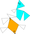
(a)

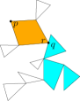
(b)

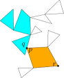
(c)

Figure 7: Rearranging a pseudo-figure by means of rooted subtree movements.

We now perform two rooted subtree movements, as illustrated in Figure 7. First, break $A_{t}^{m}$ into two rooted trees $(S,r)$ and $(T,r)$ at $r$, so that $L_{m+1}\in S$ and $L_{1},\ldots,L_{m}\in T$; move $S$ and rejoin in the form ${S}_{(r)}\wedge{}_{(q)}{T}$. Next, break this into the same two rooted subtrees $(S,r)=(S,q)$ and $(T,q)$, and move $T$ to rejoin in the form ${T}_{(q)}\wedge{}_{(p)}{S}$. In this way, the links $L_{1},\ldots,L_{m}$ are not disturbed, and $L_{m+1}$ is rooted properly, i.e. this new hinged pseudofigure is $A_{t}^{m+1}$. Repeat this procedure to finally obtain $A_{t}^{k}=A_{t}$ by rooted subtree moves, as desired. ∎

4 Continuous Motion

Theorem 6 constructs a hinged dissection that has a configuration in the form of each of the $n$ polygons. This section shows how to further refine that hinged dissection to enable it to fold continuously into each polygon while avoiding intersection among the pieces:

Theorem 7.

Any hinged figure $A$ has a refinement $B\prec A$ so that any two configurations of $B$ are reachable by a continuous non-self-intersecting motion.

Indeed, given polygons $P_{1},\ldots,P_{n}$ of equal area, Theorem 6 guarantees that there exists a hinged figure $F$ that refines each of $P_{1},\ldots,P_{n}$. By Theorem 7, there is a refinement $F^{\prime}\prec F$ that is universally reconfigurable without self-intersection. In particular, $F^{\prime}$ can continuously deform between any of the configurations induced by the $P_{i}$s. This figure $F^{\prime}$ solves the problem, proving the first sentence of Theorem 1.

To prove Theorem 7, we require two preliminary results; the first dealing with polygonal chains and slender adornments, and the other involving chainifying a given hinged figure.

4.1 Slender Adornments

Slender adornments are defined by Demaine, et al. in [CDD⁺06]. An adornment is a connected, compact region together with a line segment $ab$ (the base) lying inside the region. Furthermore, the two boundary arcs from $a$ to $b$ must be piecewise differentiable, with one-sided derivatives existing everywhere. An adornment is a slender adornment if for every point $p$ on the boundary other than $a$ and $b$, the primary inward normal(s) at $p$, namely the rays from $p$ perpendicular to the one-sided derivatives at $p$, intersect the base segment $ab$ (possibly at the endpoints). In [CDD⁺06], it is shown that chains of slender adornments cannot lock. Specifically, they show the following:

Theorem 8.

[CDD⁺06, Theorem 8] A strictly simple polygonal chain adorned with slender adornments can always be straightened or convexified.

(In a strictly simple polygonal chain, edges intersect each other only at common endpoints.) This implies that any strictly simple polygonal open chain is universally reconfigurable, because to find a continuous motion between two configurations $c_{1}$ and $c_{2}$, one may simply follow a motion from $c_{1}$ to the straightened configuration $c$, and then reverse a motion from $c_{2}$ to $c$.

4.2 Chainification

Next, we prove that any hinge figure has a refinement that is chain-like and simply adorned:

Theorem 9.

Any hinge figure $F$ has a chain-like refinement $G\prec F$ so that $G$ consists of a chain of equally-oriented obtuse triangles hinged at their acute-angled vertices.

Proof.

First we refine $F$ to consist of a tree of triangles hinged at vertices, as follows. For each $n$-sided link $L$ with $n\geq 4$, draw a collection of triangulating diagonals. Sequentially, for each such diagonal $V_{1}V_{i}$ currently in link $V=V_{1}V_{2}\ldots V_{k}$ (which may be a refinement of an original link), replace $V$ with two links $V_{1}V_{2}\ldots V_{i}$ and $V_{i}V_{i+1}\ldots V_{1}$ hinged at $V_{1}$, attaching the hinge originally at $V_{i}$ to its corresponding position on either refined piece. The resulting figure indeed consists of triangles hinged at vertices.

Next, if the resulting triangulated figure is not tree-like, we may repeatedly remove an edge from a cycle in the incidence graph (i.e. remove the corresponding link from its hinge) until the graph becomes tree-like. Call this refinement $H$.

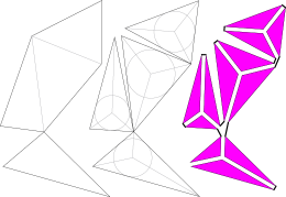
Figure 8: Chainifying a hinged figure

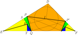
Figure 9: Refinement to hide bars from each other.

For each triangular link $ABC$ in $H$, divide $ABC$ into three triangles $AIB$, $BIC$, $CIA$, where $I$ is the incenter of $\triangle ABC$. Note that $\angle BIC=\pi-\frac{1}{2}\angle B-\frac{1}{2}\angle C>\pi-\frac{1}{2}(\angle A+\angle B+\angle C)=\frac{\pi}{2},$ i.e. $\angle BIC$ is obtuse, and likewise for the others. Finally, by hinging these obtuse triangles at the base vertices by walking around $H$’s boundary (Figure 9), we obtain the desired chain-like refinement $G$. ∎

4.3 The Final Piece of the Puzzle

We now prove Theorem 7, i.e., that any hinged figure $A$ has a universally reconfigurable refinement $B$.

Proof of Theorem 7.

As shown in Theorem 9, $A$ has a refinement $C$ consisting of obtuse triangles hinged along their bases. For each such obtuse triangle $\triangle DEF$, we create the following $7$-piece refinement (Figure 9).

Let $I$ be the incenter of triangle $DEF$, and suppose the line through $I$ perpendicular to $DI$ intersects sides $DE$ and $DF$ at $P$ and $P^{\prime}$ respectively; by obtuseness of $DIE$, $P$ lies on the interior of side $DE$, and likewise for $P^{\prime}$. Reflect $P$ over angle bisector $EI$ to $Q$; it is not hard to check that $\angle PQP^{\prime}$ = $90$. Define $R$, $S$, and $T$ as illustrated; since $PEQ$ is isosceles and acute, $R$ is inside $PEQ$. Repeat on the other side to form the $7$-piece refinement as illustrated. As the angles in all of the adornments are $90^{\circ}$ or larger, each can be easily checked to be slender. Furthermore, no bar can touch any other except at the vertices, since the bars in $DEF$ only touch the boundary of $DEF$ at single vertices, and no two bars within $DEF$ are touching. Thus, the resulting hinged figure $B$ is a strictly simple polygonal chain with slender adornments that refines $C$ (and hence refines $A$), so we are done. ∎

5 Pseudopolynomial

We now describe how to combine the preceding steps with ideas of Eppstein [Epp01] and the classical rectangle-to-rectangle dissection of Montucla [Oza78] to perform our hinged dissection using only a pseudopolynomial number of pieces, proving the second sentence of Theorem 1. In contrast to Theorem 6, we will only describe the transformation between two given polygons rather than arbitrarily many. A simple induction shows that the construction remains pseudopolynomial for a constant number of target polygons.

The idea is as follows: the inefficiency in the preceding construction is because movements may traverse the same hinges many times, leading to a recursive application of pseudosubtree movement and giving exponentially many interconnections. By performing some simplifying steps prior to subtree movement, we can instead ensure that movements are along mostly-disjoint paths so that all recursion is constant-depth.

(a)

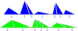
(b)

Figure 10: Equalizing the areas of two triangular chains.

To do this, given two figures, chainify them so we have two chains of triangles. We then further subdivide them so that both chains have the same number of links, and such that corresponding triangles have the same area. We do this using an idea from [Epp01]: cut the triangles from base to apex along the lines that yield the desired area, hinging at the base to maintain connectivity (see Figure 10).

Given these compatible chains, our task reduces to producing hinged dissections between each pair of equal-area triangles in such a way that the base vertices of one map to the base vertices of the other. If each individual pair of triangles requires only pseudopolynomially many pieces, we will be done.

5.1 Pseudocuts

Let $G\prec F$ be hinged figures. If we make a cut in $F$, producing $F^{\prime}$, we may not be able to directly make the same cut in $G$: attempting to do so may disconnect the figure. We give here a construction allowing us to produce an $H$ refining both $G$ and $F^{\prime}$. In keeping with earlier terminology, we call the cut in $F$ a pseudocut with respect to $G$. This operation will be useful in keeping everything pseudopolynomial.

Theorem 10.

Let $f_{1}$ and $f_{2}$ be boundary points along some link of a tree-like figure $F$. Let $F^{\prime}$ be the tree-like figure obtained by adding a straight-line cut between $f_{1}$ and $f_{2}$ and hinging at $f_{1}$, and suppose $G\prec F$. Then there exists a common refinement $H\prec G$ and $H\prec F^{\prime}$. Further, $H$ differs from $G$ only within the free region of the boundaries defined by adding the straight-line cut of $F^{\prime}$ to $G$.

Proof.

Consider the behavior of $G$ along the edge from $f_{1}$ to $f_{2}$. In $G$ the pseudocut may traverse several hinged pieces. Suppose first that the pseudocut hits no existing hinges. Let $\{h_{i}\mid 1\leq i\leq n\}$ be the points of intersection between the pseudocut and the existing edges of $G$ (so that in particular $h_{1}=f_{1}$ and $h_{n}=f_{2}$). After the cut has been made, distinguish identified vertices on each side as $h_{i}^{a}$ and $h_{i}^{b}$. We proceed inductively along the segments in $H$, beginning with $h_{1}$ to $h_{2}$ which we can easily cut and hinge exactly as in $F$.

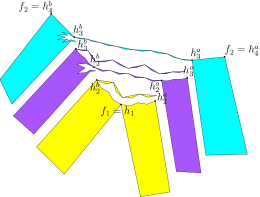
(a)

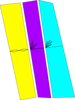
(b)

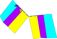
(c)

Figure 11: Making a pseudocut across existing edges

Now suppose we have already modified all segments up to $h_{i}$ to refine $F$ appropriately. Cut the segment from $h_{i}^{a}$ to $h_{i+1}$, hinging at $h_{i}^{a}$, and perform a rooted subtree movement from $h_{i}^{a}$ to $h_{i}^{b}$. We modify this movement in two ways: first, instead of tracing the entire exterior path between the two points, we use only the direct path along the cut line, with the intermediate vertices as base points of our triangle chain. Second, since this path will cross the paths used by previous segments, we reuse all base points from earlier cut-out triangles, decreasing the angle slightly to separate them; see Figure 11 for an example of this construction. Repeating this for all segments, then, we obtain the full pseudocut as desired.

Now consider the case where one or more hinges of $G$ lie on the cut edge. We only need that our inductive step can cut hinges as well as simple links. Where before our inductive transformation was based on subtree movement, for this case we will use pseudosubtree movement. Since we have already covered cutting links, we may here consider only links entirely on one side of the cut line. Treat all such links as a rooted pseudosubtree and again perform pseudosubtree movement traversing only the cut path instead of the entire figure boundary, and again reusing previous boundary triangle base points. The rest of the argument is identical.

Combining these two inductive steps allows us to produce the desired refinement across any existing configuration of the cut line in $G$, so we are done. ∎

5.2 Rectangle to Rectangle

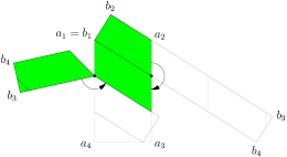
(a)

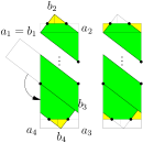
(b)

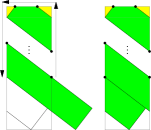
(c)

Figure 12: The stages of the rectangle-to-rectangle transformation.

The next step is to describe a pseudopolynomial hinged dissection between any two equal-area rectangles. We will compose this with our pseudocut operation in the next section to dissect between any two triangles as well. This step is heavily based on the classical (non-hinged) dissection, modified using our subtree operations to allow all operations to be hinged.

Take two rectangles of equal area, $A$ and $B$, and suppose $B$ has the smallest minimum side length. We begin by aligning both rectangles with their shorter edge on the horizontal axis and longer edge on the vertical axis, and identifying the two top left vertices. We then rotate $B$ counterclockwise until its lowest vertex is horizontally aligned with the base of $A$. Label the vertices $a_{i}$ and $b_{i}$ for $1\leq i\leq 4$, starting at the top left and moving clockwise.

At this point the horizontal cross-section of both rectangles is equal. Now, cut $B$ along edge $a_{2}a_{3}$ (the right side), hinging at the bottom of the cut, and rotate the extended portion of $B$ clockwise by $\pi$ to cover a strip of $A$. Again, cut $B$, now along the left side $a_{1}a_{4}$, hinging at the bottom, and rotate it back in, covering another horizontal strip of $A$. Continue in this way until the remaining segment of $B$ extending past $A$’s boundary is no longer enough to cover an entire horizontal strip (see Figure 12a).

Now consider the subtriangle $a_{1}b_{2}a_{2}$ of $B$. We cut it horizontally at half its height, and vertically from $b_{2}$, and rotate the resulting components out to form a rectangular cap with the same width as $A$ (see Figure 12b).

There are now two cases: either the remaining segment of $B$ extends up and left, or down and right. In the fortunate former case, we can perform the entire transformation using only classical-style manipulations: swing the extended portion back into $A$. This will give a “triangular” base, similar to the triangle that was on top of $A$, but offset horizontally and wrapping through the edge of $A$. We can make this rectangular as well by a nearly identical transformation: cut horizontally at its vertical midpoint, and vertically as shown in Figure 12b so that the pieces line up with the border of $A$ when we swing them out. A quick case analysis shows that this always works.

Now consider the remaining case where the end of $B$ extends down and to the right. We can directly reduce this to the previous case: cut $B$ along edge $a_{2}a_{3}$, hinging at the top, and use rooted subtree movement to move this subtree counterclockwise around the figure to line up with the left side of $A$ (Figure 12c). The configuration of the base is now as though $B$ had extended up and left and we rotated the extended piece down into $A$ as before, the only change being the kite sweep at the top vertex. Since this kite sweep can easily be kept above the vertical midpoint of the triangle, it doesn’t interfere with our new cuts, and the same capping strategy works without alteration.

With these steps, $B$ is transformed into a rectangle having the same area and width (and therefore same height) as $A$.

5.3 Unaltered Subtree Movement

It will be useful in the analysis to be able to perform subtree movements without modifying the subtree. This is in contrast to earlier constructions, which cut the kite tree out of the subtree being moved.

(a)

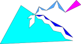
(b)

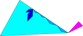
(c)

Figure 13: Moving a subtree by modifying only the parent tree

Accomplishing this is a simple modification of the earlier operation: we cut both the kite sweep and the triangle chain out of the free region of the parent subtree, and only need to alter the hinge connection points. The kite sweep will form a chain connecting at one end to the source vertex and at the other end to the subtree being moved, and the triangle chain will be a loose chain hanging from the source vertex (geometrically; it is not connected directly to the kite sweep); see Figure 13. To move the subtree, we then extend the kite sweep out, fill it in with the hanging triangle chain, and place the moving tree at the destination point.

5.4 Polygon to Polygon

With the pieces described, the transformation is simple: first, perform the equal-area chainification on both input polygons. Then convert each triangle to a rectangle using the same cutting procedure described in Figure 12b for capping the top of the rectangle. We would then like to map between the two rectangles using the rectangle-to-rectangle transformation. However, to ease analysis, we actually view the rectangle-to-rectangle transformation as being done first, and then transform the rectangles back into the original triangles by making the necessary pseudocuts as though the figures were a solid rectangle.

After these steps, we will have pairwise dissections between the triangles in the chain. In the last step, we use Unaltered Subtree Movement to adjust the hinge joints between pairs of triangles to lie on the correct boundary points. This yields a common refinement of the two triangle chains, and we are done.

5.5 Analysis

Theorem 11.

The procedure described above gives a dissection with a pseudopolynomial number of pieces.

Proof.

Since our construction worked independently on each pair of equal-area triangles, and the equal-area chainification step itself was pseudopolynomial, it suffices to show that our transformation is pseudopolynomial when applied to a single pair of triangles.

We analyze the maximum number of pieces produced by our dissection by considering the related question of the smallest possible non-zero value that can be computed at any intermediate step of the dissection. This value gives a lower bound on, for instance, the smallest distance between any two distinct vertices. If this distance is at least inverse polynomial, then a simple area argument shows that the number of pieces in the dissection is also at most polynomial.

Our task, then, is to show that the smallest non-zero value produced during the computation is indeed inverse polynomial, a question that can be dealt with almost entirely algebraically. We will use the bounds from [BFM⁺01]. Under these bounds, it suffices to show that if we view all numerical computations as a DAG, then algebraic extensions, multiplications, and divisions (by previously computed expressions) are never nested to more than constant depth, and that addition and subtraction, and multiplication or division by fixed constants, are never nested to more than linear depth. Under these constraints, if we are still able to compute the coordinates of all vertices on our figure, we will be done. For this section, refer to addition and subtraction, and multiplication and division by fixed constants, as simple arithmetic operations.

It is important in maintaining constant depth of multiplications that we never rotate the same point or vector more than a constant number of (nested) times. For instance, while for simplicity we have described adjacent kites as touching along a common angle, to attain a pseudopolynomial bound we cannot do this since each consecutive kite would give another nested rotation. Instead, whenever we need to perform a rotation, we will use a rational approximation of the angle. We can approximate an angle within an arbitrary error bound $\delta$ by using the ratios of integers that are polynomial in $1/\delta$ (for instance by solving for an appropriate Pythagorean triple). We can further ensure that we always have plenty of room for such approximations by restricting ourselves to free regions that use only half of the true available angular space, so we know that there will also be polynomial error tolerance built into any desired angles, so any single rotation will still only involve polynomial values. Kite sweeps will thus be spread out near each other but with angles ensuring they do not intersect.

Now let us consider the arithmetic/algebraic depth of the expressions produced during each step of our transformation. As mentioned above, for the purposes of analysis we consider the procedure as beginning with two equal-area rectangles and then map back to the original triangles by adding the appropriate pseudocuts.

First: When we rotate the narrower rectangle to have the same horizontal cross-section as the first, this requires a quadratic extension, as well as a constant number of multiplications and divisions to rotate all the vertices of the second rectangle.

Second: snaking the second rectangle back and forth along the first (Figure 12a) requires only additions and subtractions, since all rotations are by $\pi$. Since each pass of the rectangle must cover a strip whose height is at least the width of the second rectangle (which is at least half the height of its originating triangle), we require a linear number of passes, so the depth of simple arithmetic operations here is at most linear.

Third: Capping the triangles at the top and bottom (Figure 12b). This also requires only rotations by $\pi$, except for the extra step of finding the midpoints of the triangles’ ascent, which is just a simple arithmetic operation (division by 2).

Fourth: Moving $B$’s subtree back to the left side of $A$ (Figure 12c), if necessary. The base vertices of the triangles cut out of the border of the figure can easily be placed on rational points with low relative denominator. We will choose the inner angle of the triangles, as described earlier, to remain within the free area along the border while requiring a constant number of multiplications and divisions with suitable rational numbers. After choosing the interior angle, finding the interior vertex of a triangle can be done by intersecting its two edges, which also takes a constant number of multiplications and divisions, and can be done independently for each internal vertex to prevent nesting. Note similarly that each edge traversed by the path can be handled independently.

This still leaves the kite sweep inside the moved subtree. We can produce this from the triangle chain: each triangle pair can be made into a kite by rotating by $\pi$. Once this is done for each triangle pair, we place the kites inside the appropriate vertex by choosing approximate rotation angles as described above so the kites are non-overlapping. Each rotation requires a constant number of multiplications per vertex, but again each kite can be handled independently (and uses only expressions from its originating triangles, which were themselves computed independently of other triangle pairs), so we still preserve constant depth in our computations.

After this movement is complete, the bottom is capped identically to the previous step.

Fifth: The pseudocuts. We consider these independently. Since there are only four of them, if we show that any single pseudocut increases the simple arithmetic depth of an existing figure at most linearly, and the depth of remaining operations by at most a constant, we will be done.

Consider a single pseudocut. We know that it intersects with at most a polynomial number of edges for the simple inductive reason that so far there are only polynomially many. Furthermore, it lies in our existing algebraic extension, since all cuts were simple rational cuts with respect to the original input triangles, and the transformation to rectangles involved only rotations by $\pi$ and the single aligning rotation we performed in the first step. Thus, the coordinates defining the cut are so far at only constant computational depth.

Now, the initial vertices we need to add to our figure are the intersections of the cut line and any incident edges in the figure. Each of these can be computed independently of the rest, and each requires a constant number of multiplications and divisions. After this we need to cut out the triangle chains along the boundary of the cut, as well as the kite sweep at each joint. Once more we exploit the fact that each kite can be dealt with mostly independently: the bases of the triangles are simple rational points along the cut edges. The interior angles can be approximated as before, although now we may need to compute a polynomial number of them because of the nested triangles. However, in that case each interior angle can also be dealt with independently, so even though there are many interior vertices corresponding to each base line, they are all independently still at constant computational depth. The kite sweeps are dealt with exactly as above, a rotation by $\pi$ followed by an approximate rotation into the appropriate vertex while avoiding intersections. As all of these are still independent (relying only on the constant-depth computation to produce the appropriate base vertices, plus the constant-depth computation to produce the matching interior vertex, plus the constant-depth computation to produce a suitable rotation angle for the kite), all of this is still done in only constant depth.

Sixth: Unaltered subtree movement. This follows from the same argument as the ordinary subtree movement from the fourth step. The changes in the specific vertex used for the kite sweep make no difference to the computational depth required. Since there are only two such subtree movements, the added simple arithmetic depth is again linear, and depth of remaining operations is again constant.

Thus, we see that the computations of all steps together remain within the required bounds, and thus all vertices are indeed at least an inverse polynomial distance apart. ∎

6 Three Dimensions

We now consider hinged figures in three dimensions. A 3D hinged figure is a collection of simple polyhedra called links hinged along common positive-length edges called hinges. As before, the cyclic order of links around a hinge must remain constant.

Not every two polyhedra of equal volume have a common dissection. Dehn [Deh00] proved an invariant that must necessarily match between the two polyhedra. For example, Dehn’s invariant forbids any two distinct Platonic solids from having a common dissection. Many years later, Sydler [Syd65] proved that polyhedra $A$ and $B$ have a common dissection if and only if $A$ and $B$ have the same volume and the same Dehn invariant. Jessen [Jes68] simplified this proof by an algebraic technique and generalized the result to 4D polyhedral solids. (The 5D and higher cases remain open.) Dupont and Sah [DS90] gave another proof which illustrates further connections to algebraic structures.

Clearly, if two polyhedra have no common dissection, then they also have no common hinged dissection. We show the converse: given a common dissection of polyhedra $A$ and $B$, we can construct a common hinged dissection of $A$ and $B$. More generally, we have the following 3D analog of Theorem 6:

Theorem 12.

Given $n$ polyhedra $P_{1},\ldots,P_{n}$ of equal volume and equal Dehn invariant, there exists a hinged figure $H$ such that $H\prec P_{i}$ for $1\leq i\leq n$.

Note that our algorithms assume that the (unhinged) dissection is given. None of the proofs that Dehn’s invariant is sufficient are explicitly algorithmic, so it remains open whether one can compute a dissection when it exists. (We suspect, however, that this may be possible by suitable adaptation of an existing proof.)

All of the following definitions are 3D analogs of the definitions given in Section 2. The boundary $\partial A$ of a hinged figure $A$ is the $2$-manifold (or collection of disjoint $2$-manifolds) formed by identifying faces of links as follows: (1) for each non-hinge edge $e$ of a link $\ell$, the two faces adjacent to $e$ are connected along their common edge, and (2) for each hinge edge $e$, each pair of adjacent faces of adjacent links around $e$ are joined along their common edge. The incidence graph of a hinged figure, the notions of tree-like and chain-like, and the concept of refinement are unchanged.

The proof will be as follows: First we will describe a revised notion of free-regions for tetrahedra. Next, we illustrate the technique for moving rooted subtrees and for moving rooted pseudosubtrees, under the assumption that each link is a tetrahedron. By tetrahedralizing the links before each pseudosubtree movement, these assumptions lose nothing. The rest of the proof remains unchanged.

6.1 Defining Free Regions

We begin by defining free regions for a tetrahedron $T$. Choose an angle $\alpha$ smaller than the smallest dihedral angle of $T$’s six edges. For each face $\phi$ of $T$, let $\operatorname{free}_{T}(\phi)$ be the tetrahedron inside $T$ whose base is $\phi$ and whose base dihedral angles are $\alpha/3$.

For each edge $e$ of $T$, construct a cylinder $C_{e}$ of length $\frac{2}{3}|e|$ centered at the midpoint of $e$ with axis along $e$. Each cylinder has radius $r$, chosen small enough so that these six cylinders do not intersect, and also so that for each edge $e$, $C_{e}$ does not intersect $\operatorname{free}_{T}(\phi_{3}(e))$ and $\operatorname{free}_{T}(\phi_{4}(e))$ where $\phi_{3}(e)$ and $\phi_{4}(e)$ are the faces not adjacent to $e$.

Let $\operatorname{free}_{T}(e)$ be the wedge of $C_{e}$ of angle $\alpha/3$ centered within the dihedral angle of $T$ at $e$. By choice of $\alpha$ and $r$, $\operatorname{free}_{T}(e)$ will not intersect $\operatorname{free}_{T}(\phi)$ for any face $\phi$. These ten regions $\operatorname{free}_{T}(\cdot)$ are the desired free regions for tetrahedron $T$.

6.2 Moving Rooted Subtrees

There are two ways to join a pair of rooted subtrees $(A,a)$ and $(B,b)$ (where $a$ and $b$ are hinges or edges of their respective figures), as each edge has two possible orientations. For each rooted subtree movement of $(A,a)$ from $(B,b)$ to $(B,b^{\prime})$, we will treat $a$, $b$, and $b^{\prime}$ as oriented edges, and we will join them so that the orientations of the joined edges match.

We may now illustrate the analog of Theorem 4:

Theorem 13.

For any two tree-like hinged figures $F$ and $F^{\prime}$ related by the rooted subtree movement of $(A,a)$ from $(B,b)$ to $(B,b^{\prime})$ for oriented edges $a$, $b$, and $b^{\prime}$, there is a common refinement $G$, i.e. $G\prec F$ and $G\prec F^{\prime}$.

Proof.

The proof is in three parts, which we outline below.

We first choose the boundary path. Let $p_{a}$ be the point $1/3$ across edge $a$, and let $\phi_{0}$ be the face of $F$ to the left of edge $a$, i.e. the face so that edge $a$ traces its boundary counterclockwise (as seen from the outside). Likewise, let $p_{b^{\prime}}$ be the point $1/3$ across $b^{\prime}$, and $\phi_{1}$ the face to $b^{\prime}$’s right. Triangulate the boundary $\partial F$, and let $\gamma$ be a piecewise linear path along $\partial F$ from $p_{a}$ to $p_{b^{\prime}}$ that passes through no vertices of the triangulation, crosses each edge of each triangle orthogonally (as $\partial F$ is locally flat around each edge), begins in face $\phi_{0}$, and ends in face $\phi_{1}$. Without loss of generality, $\gamma$ does not cross itself, as loops may be eliminated. We may also assume that all turn angles of $\gamma$ are at most $90^{\circ}$, by truncating sharp turns.

Next, we thicken the boundary path. We now choose a small $\omega$ and form two paths $\gamma_{\ell}$ and $\gamma_{r}$ by offsetting $\gamma$ by a constant width of $\omega$ to the left and right, respectively. The value $\omega$ is chosen small enough to satisfy the following conditions: (1) $2\omega$ is smaller than the free-radius of $a$; (2) $2\omega<\min\{|a|,|b|\}/3$; (3) paths $\gamma_{\ell}$ and $\gamma_{r}$ have the same number of segments as $\gamma$; (4) the region $\Gamma$ between $\gamma_{\ell}$ and $\gamma_{r}$ contains no vertices of the triangulation of $\partial F$ and does not intersect itself. In essence, we have just thickened the path $\gamma$ to have width $2\omega$.

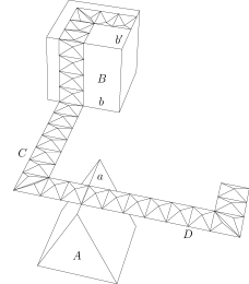
Figure 14: Moving rooted subtree $(A,a)$ from edge $b$ to edge $b^{\prime}$.

Finally, we build a pyramid chain whose base is the region $\Gamma$, as follows. We first divide $\Gamma$ into regions that will serve as the bases. Each time $\Gamma$ crosses an edge of the triangulation of $\partial F$, draw the intersection of $\Gamma$ with this edge; it intersects $\gamma$ at right angles. At each rightward turn of $\Gamma$, let $v_{r}$ be the vertex of $\gamma_{r}$ at this turn and $v_{\ell}$ that of $\gamma_{\ell}$; draw the perpendiculars from $v_{r}$ to the two edges incident with $v_{\ell}$, as well as segment $v_{r}v_{\ell}$. Perform this procedure in mirror image for all leftward turns of $\Gamma$. These drawn segments divide $\Gamma$ into rectangles and pairs of congruent right triangles. We subdivide each such rectangle of dimensions $2\omega\times s$ into $2k$ rectangles of dimensions $2\omega\times\frac{s}{2k}$, where $k$ is chosen large enough so that $\frac{s}{2k}\leq 2\omega$.

We now carve out pyramids based at each of these regions along $\Gamma$. Let $\beta$ be the free region angle at edge $a$ of $A$. For some sufficiently small $h$ (to be specified soon), form for each region $R$ along $\Gamma$ the pyramid whose base is $R$ and whose vertex is at height $h$ above the center or centroid of region $R$. These pairwise-congruent pyramids hinge along their common edges to form a chain $C$ of pyramids whose base is $\Gamma$. This chain $C$ may be folded into a “kite-sweep” of octahedra and triangular bipyramids at a common segment $t$ having length $2\omega$. If $h$ is small enough so that the total dihedral angle around $t$ is at most $\beta$, then this chain can be seen to fit within a cylindrical wedge of radius $2\omega$, angle $\beta$, height $2\omega$, and axis along $t$. Thus, carve out a chain $D$ duplicate to $C$ from $A$ based at the start of $\Gamma$ in this folded form. To ensure that $A$ is formed by simple polyhedra, we refine this link into a hinging of tetrahedra, which is possible by [Cha84].

Finally, hinge the mutilated $A$, the mutilated $B$, and chains $C$ and $D$ as illustrated in Figure 14; for the same reasons as in Theorem 4, this hinged figure forms a refinement of both $F$ and $F^{\prime}$. ∎

6.3 Moving Rooted Pseudosubtrees

A generalization of Theorem 5 follows quickly, along the lines of our generalization of Theorem 4 described in the previous subsection. It is straightforward to obtain the following result:

Theorem 14.

Take tree-like figures $F$ and $F^{\prime}$ related by the rooted-subtree movement of $(A,a)$ from $(B,b)$ to $(B,b^{\prime})$ as in Theorem 13, and suppose $G\prec F$. Then there exists a common refinement $H$ of $G$ and $F^{\prime}$.

The rest of the proof of Theorem 12 follows the proof of Theorem 6 unchanged. We obtain Theorem 2 as an immediate corollary.

6.4 Higher Dimensions

We believe, although we have not verified, that our techniques generalize further to refining dissections of polyhedral solids in arbitrary dimensions into equivalent hinged dissections. Again we obtain only configurations, not folding motions, for each desired polyhedral solid. Also, it is unknown when common (unhinged) dissections exist in 5D and higher [DS90], although the solution in 4D is again the Dehn invariant [Jes68].

References

- [AN98] Jin Akiyama and Gisaku Nakamura. Dudeney dissection of polygons. In Revised Papers from the Japan Conference on Discrete and Computational Geometry, volume 1763 of Lecture Notes in Computer Science, pages 14–29, Tokyo, Japan, December 1998.
- [ANN+03] Jin Akiyama, Gisaku Nakamura, Akihiro Nozaki, Ken’ichi Ozawa, and Toshinori Sakai. The optimality of a certain purely recursive dissection for a sequentially -divisible square. Computational Geometry: Theory and Applications, 24(1):27–39, 2003.
- [BFM+01] Christoph Burnikel, Stefan Funke, Kurt Mehlhorn, Stefan Schirra, and Susanne Schmitt. A separation bound for real algebraic expressions. In Proceedings of the 9th Annual European Symposium on Algorithms, volume 2161 of Lecture Notes in Computer Science, pages 254–265, Aarhus, Denmark, 2001.
- [Bol33] Farkas Bolyai. Tentamen juventutem studiosam in elementa matheseos purae, elementaris ac sublimioris, methodo intuitiva, evidentiaque huic propria, introducendi. Typis Collegii Refomatorum per Josephum et Simeonem Kali, Maros Vásárhely, 1832–1833.
- [CDD+06] Robert Connelly, Erik D. Demaine, Martin L. Demaine, Sándor Fekete, Stefan Langerman, Joseph S. B. Mitchell, Ares Ribó, and Günter Rote. Locked and unlocked chains of planar shapes. In Proceedings of the 22nd Annual ACM Symposium on Computational Geometry, pages 61–70, Sedona, Arizona, June 2006.
- [CDR03] Robert Connelly, Erik D. Demaine, and Günter Rote. Straightening polygonal arcs and convexifying polygonal cycles. Discrete & Computational Geometry, 30(2):205–239, September 2003.
- [Cha84] Bernard Chazelle. Convex partitions of polyhedra: a lower bound and worst-case optimal algorithm. SIAM Journal on Computing, 13(3):488–507, 1984.
- [CKU99] Jurek Czyzowicz, Evangelos Kranakis, and Jorge Urrutia. Dissections, cuts, and triangulations. In Proceedings of the 11th Canadian Conference on Computational Geometry, Vancouver, Canada, August 1999. http://www.cs.ubc.ca/conferences/CCCG/elec˙proc/c33.ps.gz.
- [Coh75] M. J. Cohn. Economical triangle-square dissection. Geometriae Dedicata, 3:447–467, 1975.
- [DDE+05] Erik D. Demaine, Martin L. Demaine, David Eppstein, Greg N. Frederickson, and Erich Friedman. Hinged dissection of polyominoes and polyforms. Computational Geometry: Theory and Applications, 31(3):237–262, June 2005.
- [DDLS05] Erik D. Demaine, Martin L. Demaine, Jeffrey F. Lindy, and Diane L. Souvaine. Hinged dissection of polypolyhedra. In Proceedings of the 9th Workshop on Algorithms and Data Structures, volume 3608 of Lecture Notes in Computer Science, pages 205–217, Waterloo, Canada, August 2005.
- [Deh00] M. Dehn. Über den Rauminhalt. Nachrichten von der Gesellschaft der Wissenschaften zu Göttingen, Mathematisch-Physikalische Klasse, pages 345–354, 1900. Later published in Mathematische Annalen 55:465–478, 1902.
- [DMO03] Erik D. Demaine, Joseph S.B. Mitchell, and Joseph O’Rourke. Problem 47: Hinged dissections. In The Open Problems Project. March 2003. http://www.cs.smith.edu/~orourke/TOPP/P47.html.
- [DS90] Johan L. Dupont and Chih-Han Sah. Homology of Euclidean groups of motions made discrete and Euclidean scissors congruences. Acta Mathematica, 164(1):1–27, 1990.
- [Dud02] Henry E. Dudeney. Puzzles and prizes. Weekly Dispatch, 1902. The puzzle appeared in the April 6 issue of this column. An unusual discussion followed on April 20, and the solution appeared on May 4.
- [Epp01] David Eppstein. Hinged kite mirror dissection. arXiv:cs.CG/0106032, June 2001. http://arXiv.org/abs/cs.CG/0106032.
- [Fre97] Greg N. Frederickson. Dissections: Plane and Fancy. Cambridge University Press, November 1997.
- [Fre02] Greg N. Frederickson. Hinged Dissections: Swinging & Twisting. Cambridge University Press, August 2002.
- [Ger33] P. Gerwien. Zerschneidung jeder beliebigen Anzahl von gleichen geradlinigen Figuren in dieselben Stücke. Journal für die reine und angewandte Mathematik (Crelle’s Journal), 10:228–234 and Taf. III, 1833.
- [Gri04] Saul Griffith. Growing Machines. PhD thesis, Media Laboratory, Massachusetts Institute of Technology, September 2004.
- [Jes68] Børge Jessen. The algebra of polyhedra and the Dehn-Sydler theorem. Mathematica Scandinavica, 22:241–256, 1968.
- [Kel64] Philip Kelland. On superposition. part II. Transactions of the Royal Society of Edinburgh, 33:471–473 and plate XX, 1864.
- [KKU00] Evangelos Kranakis, Danny Krizanc, and Jorge Urrutia. Efficient regular polygon dissections. Geometriae Dedicata, 80:247–262, 2000.
- [Lem90] Don Lemon. The Illustrated Book of Puzzles. Saxon, London, 1890.
- [Lin72] Harry Lindgren. Recreational Problems in Geometric Dissections and How to Solve Them. Dover Publications, Inc., 1972. Revised and enlarged by Greg Frederickson.
- [Low14] Mr. Lowry. Solution to question 269, [proposed] by Mr. W. Wallace. In T. Leybourn, editor, Mathematical Repository, volume 3, part 1, pages 44–46. W. Glendinning, London, 1814.
- [Mad79] Joseph S. Madachy. Geometric dissections. In Madachy’s Mathematical Recreations, chapter 1, pages 15–33. Dover Publications, 1979. Reprint of Mathematics on Vacation, Scribner, 1975.
- [MTW+02] Chengde Mao, Venkat R. Thallidi, Daniel B. Wolfe, Sue Whitesides, and George M. Whitesides. Dissections: Self-assembled aggregates that spontaneously reconfigure their structures when their environment changes. Journal of the American Chemical Society, 124:14508–14509, 2002.
- [O’R02] Joseph O’Rourke. Computational geometry column 44. International Journal of Computational Geometry and Applications, 13(3):273–275, 2002.
- [Oza78] Jacques Ozanam. Récréations Mathématiques et Physiques, pages 297–302. Claude Antoine Jombert, fils, Paris, 1778. According to [Fre97], this material was added by Jean Montucla under the pseudonym M. de Chanla.
- [Pan49] André-J. Panckoucke. Les Amusemens Mathématiques. Chez André-Joseph Panckoucke, Lille, 1749.
- [RBKV02] Daniela Rus, Zack Butler, Keith Kotay, and Marsette Vona. Self-reconfiguring robots. Communications of the ACM, 45(3):39–45, 2002.
- [Str05] Ileana Streinu. Pseudo-triangulations, rigidity and motion planning. Discrete & Computational Geometry, 34(4):587–635, November 2005.
- [Syd65] J.-P. Sydler. Conditions nécessaires et suffisantes pour l’équivalence des polyèdres de l’espace euclidien à trois dimensions. Commentarii Mathematici Helvetici, 40:43–80, 1965.
- [Wal31] William Wallace, editor. Elements of Geometry. Bell & Bradfute, Edinburgh, 8th edition, 1831.