On weak and strong magnetohydrodynamic turbulence

Abstract

Recent numerical and observational studies contain conflicting reports on the spectrum of magnetohydrodynamic turbulence. In an attempt to clarify the issue we investigate anisotropic incompressible magnetohydrodynamic turbulence with a strong guide field $B_{0}$. We perform numerical simulations of the reduced MHD equations in a special setting that allows us to elucidate the transition between weak and strong turbulent regimes. Denote $k_{\|}$, $k_{\perp}$ characteristic field-parallel and field-perpendicular wavenumbers of the fluctuations, and $b_{\lambda}$ the fluctuating field at the scale $\lambda\sim 1/k_{\perp}$. We find that when the critical balance condition, $k_{\|}B_{0}\sim k_{\perp}b_{\lambda}$, is satisfied, the turbulence is strong, and the energy spectrum is $E(k_{\perp})\propto k^{-3/2}_{\perp}$. As the $k_{\|}$ width of the spectrum increases, the turbulence rapidly becomes weaker, and in the limit $k_{\|}B_{0}\gg k_{\perp}b_{\lambda}$, the spectrum approaches $E(k_{\perp})\propto k_{\perp}^{-2}$. The observed sensitivity of the spectrum to the balance of linear and nonlinear interactions may explain the conflicting numerical and observational findings where this balance condition is not well controlled.

1. Introduction

In this Letter we investigate homogeneous and steadily driven incompressible magnetohydrodynamic (MHD) turbulence. In practical applications, such as fusion devices, solar wind, and interstellar medium, turbulence is driven by various large-scale instabilities, and turbulent energy is then spread over a broad range of spatial scales due to nonlinear interactions until small dissipative scales are reached where the energy is removed from the system. In the interval of scales between the injection and dissipation regions turbulence properties are thought to be universal (e.g., Frisch, 1995; Biskamp, 2003).

The MHD equations describing the evolution of magnetic and velocity fluctuations ${\bf b}(\bf x,t)$ and ${\bf v}(\bf x,t)$ in the presence of a guide field ${\bf B_{0}}$ can be represented in the so-called Elsässer variables ${\bf z}^{\pm}={\bf v}\pm{\bf b}$:

$$\partial_{t}{\bf z}^{\pm}\mp({\bf V}_{A}\cdot\nabla){\bf z}^{\pm}+({\bf z}^{\mp}\cdot\nabla){\bf z}^{\pm}=-\nabla P+{\bf f},$$ (1)

where ${\bf V}_{A}={\bf B}_{0}/\sqrt{4\pi\rho}$ is the Alfvén velocity, $\rho$ is the fluid density, $P$ is the pressure that is determined from the incompressibility condition, $\nabla\cdot{\bf z}^{\pm}=0$, ${\bf f}$ represents a large-scale forcing, and we omit the terms representing small viscosity and resistivity. The linear term on the left-hand side of equations (1), $({\bf V}_{A}\cdot\nabla){\bf z}^{\pm}$, is responsible for advection of the $z^{+}$ and $z^{-}$ wave packets, with the Alfvén velocity along the guide field. The nonlinear term, $({\bf z}^{\mp}\cdot\nabla){\bf z}^{\pm}$, describes the interaction of turbulent fluctuations, and it is responsible for the energy transfer among different spatial scales. The nonlinear term is considered small if

$$k_{\|}B_{0}\gg k_{\perp}b_{\lambda},$$ (2)

where $k_{\|}$ and $k_{\perp}$ are typical field-parallel and field-perpendicular wavenumbers of the fluctuations’ spectrum, and $b_{\lambda}$ ($\ll B_{0}$) is the typical magnitude of fluctuations at the scale $\lambda\sim 1/k_{\perp}$. This regime is referred to as “weak turbulence.”

The regime when the nonlinear term in not formally small will be called “strong turbulence.” One can argue that in strong turbulence the following critical balance condition should be maintained at all scales (Goldreich & Sridhar, 1995):

$$k_{\|}B_{0}\sim k_{\perp}b_{\lambda}.$$ (3)

Indeed, during the characteristic time of nonlinear interaction, $\tau_{N}\sim 1/(k_{\perp}b_{\lambda})$, the fluctuations become correlated along the guide field up to a distance $l_{\|}\sim V_{A}\tau_{N}$. This causality condition ensures the critical balance (3). Depending on the way turbulence is excited, it satisfies either condition (2) or (3) in a certain range of scales.

Recent numerical simulations and analytic modeling suggest that in the case of strong turbulence (3), the field-perpendicular energy spectrum is $E(k_{\perp})\propto k_{\perp}^{-3/2}$ (Maron & Goldreich, 2001; Müller & Grappin, 2005; Boldyrev, 2005, 2006; Mason et al., 2006, 2007). However, geophysical and astrophysical observations often exhibit somewhat steeper spectra (e.g., Goldstein et al., 1995; Bale, et al, 2005). This raises the question of to what extent such systems can be described in the framework of MHD turbulence.

In the present work we conduct direct numerical simulations of reduced MHD equations, driven by a force with varying $k_{\|}$ spectral width. This provides a unifying numerical setting allowing one to address the regimes of weak and strong turbulence in the same framework. We observe that when the critical balance (3) is satisfied, the spectrum of strong MHD turbulence is close to $-3/2$. When the critical balance condition (3) is even slightly broken, the spectrum steepens. As the weak turbulence condition (2) becomes better satisfied, the spectral exponent approaches $-2$ in accord with the theory of weak turbulence (Ng & Bhattacharjee, 1996; Galtier et al., 2000). The observed sensitivity of the spectrum to the forcing details may explain conflicting results of numerical and astrophysical observations, where the spectral properties of forcing are either not well controlled or not well known.

According to the standard derivation (e.g., Biskamp, 2003), the reduced MHD equations are valid in the region $k_{\perp}\gg k_{\|}$; therefore, their applicability in the strong turbulence regime (3) is justified. Their applicability in the weak turbulence regime (2), however, requires an explanation, which we provide in the following sections.

2. Weak MHD Turbulence.

When the condition (2) is satisfied, one may assume that turbulence consists of shear-Alfvén and pseudo-Alfvén waves, weakly interacting with each other. In the absence of nonlinear interaction, the waves would have random phases, and the Gaussian rule could be applied to express their higher order correlation functions through the second-order ones. Galtier et al. (2000) developed a perturbative theory of weak MHD turbulence based on such random phase approximation. By expanding the MHD eq. (1) up to the second order in the nonlinear interaction and using the Gaussian rule to split the fourth-order correlators, they derived a closed system of kinetic equations governing the wave energy spectra.

These equations demonstrate that wave energy cascades in the Fourier space in the direction of large $k_{\perp}$, and the universal spectrum of wave turbulence is established in the region $k_{\perp}\gg k_{\|}$. In this limit the dynamics of the shear-Alfvén waves decouple from the dynamics of the pseudo-Alfvén waves, and the pseudo-Alfvén waves are passively scattered by the shear-Alfvén ones. The kinetic equation for the energy spectrum of shear-Alfvén waves, $e({\bf k},t)$, derived by Galtier et al. (2000), then reads:

$$\partial_{t}e({\bf k})=\int M_{{\bf k},{\bf p}{\bf q}}e({\bf q})[e({\bf p})-e({\bf k})]\delta(q_{\|})d_{\bf k,pq}$$ (4)

In this expression, the interaction kernel is $M_{{\bf k},{\bf p}{\bf q}}=({\pi}/{V_{A}}){({\bf k}_{\perp}\times{\bf q}_{\perp})^{2}({\bf k}_{\perp}\cdot{\bf p}_{\perp})^{2}}/({k_{\perp}^{2}q_{\perp}^{2}p_{\perp}^{2}})$, and we adopt the shorthand notation $d_{\bf k,pq}\equiv\delta({\bf k}-{\bf p}-{\bf q})\,d^{3}p\,d^{3}q$. The phase-volume compensated energy spectrum is then calculated as $E({\bf k},t)dk_{\|}\,dk_{\perp}=e({\bf k},t)k_{\perp}dk_{\|}\,dk_{\perp}$. The stationary solution of equation (4) was found analytically and verified numerically in (Galtier et al., 2000). It has the general form $E({\bf k})=f(k_{\|})k_{\perp}^{-2}$, where $f(k_{\|})$ is an arbitrary function that is smooth at $k_{\|}=0$.

It should be noted, however, that the derivation of (4) based on the weak interaction approximation is not rigorous. As follows from Eq. (4), only the $q_{\|}=0$ components of the energy spectrum $e({\bf q})$ are responsible for the energy transfer. However, if we apply Eq. (4) to these dynamically important components themselves, that is, if we set $k_{\|}=0$ in (4), we observe an inconsistency. Indeed, the perturbative approach implies that the linear frequencies of the waves are much larger than the frequency of their nonlinear interaction. The nonlinear interaction in (4) remains nonzero as $k_{\|}\to 0$ while the linear frequency of the corresponding Alfvén modes, $\omega_{k}=k_{\|}V_{A}$, vanishes. Therefore, as shown by Galtier et al. (2000), the additional assumption of smoothness of the function $f(k_{\|})$ at $k_{\|}=0$ is crucial for deriving the spectrum $E({\bf k})\propto k_{\perp}^{-2}$.

A definitive numerical verification of such a spectrum seems therefore desirable. While numerical integration of a scattering model based on MHD equations expanded up to the second order in nonlinear interaction does reproduce the $-2$ exponent (Bhattacharjee & Ng, 2001; Ng et al., 2003), this spectrum has not yet been confirmed in direct numerical simulations of systems (1). The major problem faced by such simulations is to simultaneously satisfy the two conditions, $k_{\perp}\gg k_{\|}$ and $k_{\|}B_{0}\gg k_{\perp}b_{\lambda}$, which is hard to achieve with present-day computing power. In the next section we discuss a numerical setting in which the spectrum of weak turbulence can be verified.

3. Model equations.

An important fact concerning Eq. (4) was emphasized by Galtier & Chandran (2006). They noted that there exists a dynamical system that leads to exactly the same kinetic equation (4) in the weak turbulence regime (2), without any additional restrictions on $k_{\perp}$ and $k_{\|}$. To derive this system, we note that in the universal regime where Eq. (4) is applicable, the polarization vectors of the pseudo-Alfvén modes are almost parallel to the guide field. One can therefore consider a system where such modes are eliminated for arbitrary ${\bf k}$ by restricting the initial MHD system to field-perpendicular fluctuations, ${\tilde{\bf z}}^{\pm}$:

$$\displaystyle\partial_{t}{\tilde{\bf z}}^{\pm}\mp({\bf V}_{A}\cdot\nabla){\tilde{\bf z}}^{\pm}+({\tilde{\bf z}}^{\mp}\cdot\nabla){\tilde{\bf z}}^{\pm} = -\nabla_{\perp}P+\frac{1}{Re}\nabla^{2}{\tilde{\bf z}}^{\pm}+{\tilde{\bf f}},$$

$$\nabla\cdot{\tilde{\bf z}}^{\pm} = 0.$$ (5)

The fluctuating fields here have only two vector components, ${\tilde{\bf z}}^{\pm}=\{{\tilde{z}}^{\pm}_{1},{\tilde{z}}^{\pm}_{2},0\}$, but depend on all three spatial coordinates. Although system (3) is not presented in (Galtier & Chandran, 2006), their analysis of (1) is equivalent to solving such a system. Formally, system (3) is equivalent to the reduced MHD equations (e.g., Biskamp, 2003; Shebalin et al., 1983). The principal difference is in the limits of validity: the reduced MHD model is applicable only for $k_{\perp}\gg k_{\|}$, while we consider system (3) without any restrictions.

Within the formalism of the weak turbulence theory both systems (1) and (3) lead to the same kinetic equation (4) for the shear-Alfvén turbulence. We thus conclude that the wave energy spectrum obtained from the full MHD system (1) under the assumption $k_{\perp}\gg k_{\|}$ should coincide with the spectrum obtained from the restricted system (3), where the condition $k_{\perp}\gg k_{\|}$ is not required. On the other hand, strong turbulence is expected to develop when $k_{\|}B_{0}\sim k_{\perp}b_{\lambda}$, which is precisely the domain in which reduced MHD provides a good approximation of the full MHD model. This opens an effective way for numerical investigation of both strong and weak MHD turbulence in the same framework, which is the goal of the present Letter.

4. Numerical method and results.

We solve numerically the restricted MHD model (3) using a fully dealiased pseudo-spectral technique in a periodic box that is elongated along the guide field ${\bf B}_{0}$ with aspect ratio $2\pi:2\pi:L_{z}$. The random force ${\tilde{\bf f}}$ has no component along $z$, it is solenoidal in the $x-y$ plane and its Fourier coefficients outside the range $1\leq k_{\perp}\leq 2$, $(2\pi/L_{z})\leq k_{\|}\leq(2\pi/L_{z})n_{z}$ are zero, where integer $n_{z}$ determines the width of the force spectrum in $k_{\|}$. The Fourier coefficients inside that range are Gaussian random numbers with amplitude chosen so that the resulting rms velocity fluctuations are of order unity. The individual random values are refreshed independently at time intervals $\tau=0.1~{}L_{\perp}/(2\pi U_{rms})$. The parameters $n_{z}$ and $L_{z}$ control the degree to which condition (2) or (3) is satisfied at the forcing scale. Note that we do not drive the $k_{\|}=0$ modes but allow them to be generated by nonlinear interactions. The Reynolds number is defined as $Re=U_{rms}(L_{\perp}/2\pi)/\nu$, where $L_{\perp}$ $(=2\pi)$ is the field-perpendicular box size, $\nu$ is fluid viscosity, and $U_{rms}$ $(\sim 1)$ is the rms value of velocity fluctuations. In our case magnetic resistivity and fluid viscosity are the same, $\nu=\eta$. The system is evolved until a stationary state is reached, as determined by the time evolution of the total energy of the fluctuations. A typical run produces from 30 to 60 snapshots. The field-perpendicular energy spectrum is obtained by averaging the angle-integrated Fourier spectrum, $E(k_{\perp})=0.5\langle|{\bf v}({\bf k_{\perp}})|^{2}\rangle k_{\perp}+0.5\langle|{\bf b}({\bf k_{\perp}})|^{2}\rangle k_{\perp}$, over field-perpendicular planes in all snapshots.

Figure 1.— The field-perpendicular energy spectrum $E(k_{\perp})$ of MHD turbulence, calculated by direct numerical integration of (3). The presented cases correspond, from bottom to top, to $\kappa=1/6,\,1/5,\,2/5,\,4/5,\,8/5,\,16/5$. For clarity, the curves in the top panel are arbitrarily offset in the vertical direction.

We performed a series of simulations for $B_{0}=5$, $L_{z}=5L_{\perp}$ and $n_{z}=1,\,2,\,4,\,8,\,16$. We used the resolution $256^{3}$ mesh points in these simulations (and $Re=800$), except for the case $n_{z}=16$, where the resolution was $512\times 512\times 256$ (and $Re_{\perp}=2000$). We also performed a simulation with $B_{0}=5$, $L_{z}=6L_{\perp}$, and $n_{z}=1$ and the resolution $512\times 512\times 256$ (and $Re_{\perp}=2000$). Fig. 1 shows the field-perpendicular energy spectra for each run. All the runs have different values of parameter $\kappa\equiv(2\pi/L_{z})n_{z}$ that measures deviation from the critical balance (3) condition.

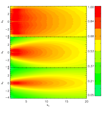
Figure 2.— Contour plots of the anisotropic energy spectra for the cases $\kappa=1/6$ (bottom), $\kappa=4/5$ (center), and $\kappa=16/5$ (top). The colors represent energy in a log scale, normalized to the energy of the most dominant large-scale mode.

We found that as the spectral width of the forcing along $k_{\|}$ increases, higher and higher frequency modes of the velocity and magnetic fields are excited. For run $\kappa=1/6$, all the forced modes have linear frequency $\omega=k_{\|}B_{0}\approx 1$, which corresponds to a critically balanced forcing. In this case, the spectrum is $E(k_{\perp})\propto k_{\perp}^{-3/2}$. This result is consistent with recent numerical simulation of full MHD by Mason et al. (2007), since the reduced MHD system approximates the full MHD system when the critical balance condition is satisfied. As we increase the parameter $\kappa$, we break the critical balance condition at the forcing scales. As a result, the spectrum monotonically steepens from $-3/2$ in the strong turbulence case to $-2$ in the weak turbulence case, as shown in Fig. 1.

Fig. 2 shows isocontours of the full energy spectrum $E(k_{\|},k_{\perp})$ as a function of $k_{\perp}$ and $k_{\|}$ for the three typical cases $\kappa=1/6,\,4/5,\,16/5$. The bottom frame presents the energy distribution for the case $\kappa=1/6$, where the random force preserves the critical balance. As the cascade continues deeper into the inertial range, higher frequency modes $\omega=k_{\|}B_{0}$ are generated by virtue of nonlinear interactions, just enough to maintain the critical balance condition at all scales, and establish a strong turbulence spectrum. As the frequency of the forced Alfvén modes increases in the cases $\kappa=(2,\dots,16)/5$, the parallel cascade is slightly inhibited as the weaker interaction among the large scale Alfvén modes dominates the energy transfer to smaller scales, resulting in a steepening of the field-perpendicular energy spectrum. This can be seen in the middle and top frames in Fig. 2, where the distribution of energy becomes more and more elongated along $k_{\perp}$ rather than $k_{\|}$.

5. Discussion.

Our numerical results demonstrate that if the energy spectrum has a limited extent, increasing the $k_{\|}$ width of the forcing spectrum leads to the energy spectrum of weak turbulence $\propto k_{\perp}^{-2}$. If however the $k_{\|}$ width of the forcing is limited, but we can achieve arbitrarily high resolution in the $k_{\perp}$ direction, the interaction between Alfvén modes will eventually become strong enough to satisfy critical balance and establish a strong turbulence spectrum.

This is partly supported by the following derivation. It can be proved that turbulent fluctuations described by system (3) satisfy the exact relation:

$$\langle\delta{\tilde{z}}^{\pm}_{l}(\delta{\tilde{\bf z}}^{\mp})^{2}\rangle=-2\epsilon^{\mp}r_{\perp},$$ (6)

where $\delta{\tilde{\bf z}}^{\pm}={\tilde{\bf z}}^{\pm}({\bf x}+{\bf r}_{\perp})-{\tilde{\bf z}}^{\pm}({\bf x})$, and $\delta{\tilde{z}}^{\pm}_{l}=\delta{\tilde{\bf z}}^{\pm}\cdot{\bf r}_{\perp}/r_{\perp}$ is the longitudinal component of $\delta{\tilde{\bf z}}^{\pm}$. Averaging is taken over the statistical ensemble, or over time and spatial position x. In this formula, $\epsilon^{\pm}$ are the constant rates of ${\tilde{z}}^{+}$ and ${\tilde{z}}^{-}$ energy dissipation. In the isotropic case, that is, without the guide field, the relation analogous to (6) was derived by Politano & Pouquet (1998). We now prove the following general inequality:

$$\langle\delta{\tilde{z}}^{\pm}_{l}(\delta{\tilde{\bf z}}^{\mp})^{2}\rangle^{2}\leq\langle(\delta{\tilde{\bf z}}^{\pm})^{2}\rangle\langle(\delta{\tilde{\bf z}}^{\mp})^{4}\rangle.$$ (7)

The first step is to use the Schwartz inequality, $\langle\delta{\tilde{z}}^{\pm}_{l}(\delta{\tilde{\bf z}}^{\mp})^{2}\rangle^{2}\leq\langle(\delta{\tilde{z}}_{l}^{\pm})^{2}\rangle\langle(\delta{\tilde{\bf z}}^{\mp})^{4}\rangle$; the second step is to note that $(\delta{\tilde{z}}^{\pm}_{l})^{2}\leq(\delta{\tilde{\bf z}}^{\pm})^{2}$, which completes the proof.

Both sides in the expression (7) have finite limits as viscosity and resistivity go to zero. In the inertial interval, the correlation functions on the right-hand side of this expression have a power-law behavior, that is, $\langle(\delta{\tilde{\bf z}}^{\pm})^{2}\rangle\propto r_{\perp}^{{\zeta}_{2}}$ and $\langle(\delta{\tilde{\bf z}}^{\pm})^{4}\rangle\propto r_{\perp}^{{\zeta}_{4}}$ (we assume statistical symmetry between ${\tilde{\bf z}}^{+}$ and ${\tilde{\bf z}}^{-}$). Since the left hand side of (7) scales as $\propto r_{\perp}^{2}$, and the inequality should hold for arbitrarily small $r_{\perp}$, we obtain the exact result

$$\zeta_{2}+\zeta_{4}\leq 2.$$ (8)

This inequality is useful for evaluation of these exponents from numerical simulations or experiments since the ratio of these exponents is well measured by the method of extended self-similarity (Benzi et al., 1993). The inequality (8) then provides a boundary on the turbulence energy spectrum that is related to the second-order scaling exponent as $E(k_{\perp})\propto k_{\perp}^{-1-\zeta_{2}}.$ In our case, the scaling exponent ${\zeta}_{4}$ is usually close to $2{\zeta}_{2}$ within small intermittency corrections, which can be checked numerically (e.g., Müller et al., 2003). Inequality (8) then implies that $3{\zeta}_{2}\leq 2$, and, therefore, the field-perpendicular energy spectrum cannot be essentially steeper than $E(k_{\perp})\propto k^{-5/3}_{\perp}$ in the limit $k_{\perp}\to\infty$.

Note, however, that in our numerical findings the spectral exponent $-5/3$ is not distinguished in any way; rather, the field-perpendicular energy spectrum of strong MHD turbulence is flatter and closer to $-3/2$. This is consistent with recent results of Müller & Grappin (2005); Mason et al. (2007) and also with high-resolution simulations of isotropic MHD turbulence by Haugen et al. (2003); Mininni & Pouquet (2007). Astrophysical observations of the solar wind and of the interstellar medium reveal the presence of MHD turbulence, and find support for both $-5/3$ and $-3/2$ spectral exponents (e.g., Goldstein et al., 1995; Goldstein & Roberts, 1999; Bale, et al, 2005; Borovsky, 2006; Podesta et al., 2006; Smirnova et al., 2006). However, statistics of such data are often not good enough to distinguish between “$-5/3$” and “$-3/2$” with confidence. On the numerical side, simulations of MHD turbulence in the framework of reduced MHD were performed in many works (e.g., Dmitruk et al., 2003; Gomez et al., 2005; Rapazzo et al., 2007); however, either the simulation domain was not anisotropic to ensure the critical balance condition (3), or the driving force was not spatially homogeneous, for example, applied at the boundary of the domain.

Our results suggest that the interpretation of observational and numerical results may be obscured if the $k_{\|}$ and $k_{\perp}$ structure of the spectrum is either not well measured or not well controlled, in which case it is hard to deduce whether the field-parallel dynamics have been captured and whether the universal regime of MHD turbulence has been established.

References

- Bale, et al (2005) Bale, S. D., Kellog, P. J., Mozer, F. S., Hornbury, T. S., & Reme, H., Phys. Rev. Lett., 94 (2005) 215002.
- Benzi et al. (1993) Benzi, R., Ciliberto, S., Tripiccione, R., Baudet, C., Massaioli, F., and Succi, S. (1993) Phys. Rev. E 48 R29.
- Bhattacharjee & Ng (2001) Bhattacharjee, A. & Ng, C. S., ApJ 548 (2001) 318.
- Biskamp (2003) Biskamp, D., 2003, Magnetohydrodynamic Turbulence. (Cambridge University Press, Cambridge).
- Boldyrev (2005) Boldyrev, S., ApJ 626 (2005) L37.
- Boldyrev (2006) Boldyrev, S., Phys. Rev. Lett. 96 (2006) 115002.
- Borovsky (2006) Borovsky, J., J. Geophys. Res. (2006) submitted.
- Dmitruk et al. (2003) Dmitruk, P., Gomez, D., Matthaeus, W., Phys. Plasmas, 10 (2003) 3584.
- Frisch (1995) Frisch, U., 1995, Turbulence. (Cambridge University Press, Cambridge).
- Galtier et al. (2000) Galtier, S., Nazarenko, S. V., Newell, A. C., & Pouquet, A., J. Plasma Physics 63 (2000) 447.
- Galtier & Chandran (2006) Galtier, S. & Chandran, B.D.G., Phys. Plasmas, 13 114505 (2006).
- Goldreich & Sridhar (1995) Goldreich, P. & Sridhar, S., ApJ 438 (1995) 763.
- Goldstein & Roberts (1999) Goldstein, M. L.; Roberts, D. A., Phys. Plasmas, 6 (1999) 4154.
- Goldstein et al. (1995) Goldstein, D. A. Roberts, D. A., & Matthaeus, W. H., Annu. Rev. Astron. Astrophys. 33 (1995) 283.
- Gomez et al. (2005) Gomez, D. O., Mininni, P.D. & Dmitruk, P., Physica Scripta T 116 (2005) 123.
- Haugen et al. (2003) Haugen, N.E.L., Brandenburg, A. & Dobler, W., ApJ 597 (2003) L141.
- Maron & Goldreich (2001) Maron, J., & Goldreich, P., ApJ 554 (2001) 1175.
- Mason et al. (2006) Mason, J., Cattaneo, F., & Boldyrev, S., Phys. Rev. Lett, 97 (2006) 255002.
- Mason et al. (2007) Mason, J., Cattaneo, F., & Boldyrev, S., arXiv:0706.2003 (2007).
- Mininni & Pouquet (2007) Mininni P.D. & Pouquet, A., arXiv:0707.3620 (2007).
- Müller et al. (2003) Müller, W.-C., Biskamp, D., & Grappin, R., Phys. Rev. E 67 (2003) 066302.
- Müller & Grappin (2005) Müller, W.-C. & Grappin, R., Phys. Rev. Lett., 95 (2005) 114502.
- Newell et al. (2001) Newell, A. C., Nazarenko, S., & Biven, L., Physica D 152-153 (2001) 520.
- Ng & Bhattacharjee (1996) Ng, C. S. & Bhattacharjee, A., ApJ 465 (1996) 845.
- Ng et al. (2003) Ng, C. S., Bhattacharjee, A., Germashewski, K. & Galtier, S., Phys. Plasmas 10 (2003) 1954.
- Podesta et al. (2006) Podesta, J. J., Roberts, D. A., & Goldstein, M. L., J.Geophys. Res. 111 (2006) A10109.
- Politano & Pouquet (1998) Politano, H. & Pouquet, A., Geophys. Res. Lett. 25 (1998) 273.
- Rapazzo et al. (2007) Rappazo, A. F., Velli, M., Einaudi, G., & Dalburgh, R. B., ApJ 657 (2007) L47.
- Shebalin et al. (1983) Shebalin, J. V., Matthaeus, W. H. & Montgomery, D., J. Plasma Physics, 29 (1983) 525.
- Smirnova et al. (2006) Smirnova, T. V., Gwinn, C. R., & Shishov, V. I., Astron. Astrophys. 453 (2006) 601.
- Zakharov et al. (1992) Zakharov, V. E., L’vov, V. S. & Falkovich, G., Kolmogorov Spectra of Turbulence (Springer, Berlin, 1992).