Theoretical analysis of a single and double reflection atom interferometer in a weakly-confining magnetic trap

Abstract

The operation of a BEC based atom interferometer, where the atoms are held in a weakly-confining magnetic trap and manipulated with counter-propagating laser beams, is analyzed. A simple analytic model is developed to describe the dynamics of the interferometer. It is used to find the regions of parameter space with high and low contrast of the interference fringes for both single and double reflection interferometers. We demonstrate that for a double reflection interferometer the coherence time can be increased by shifting the recombination time. The theory is compared with recent experimental realizations of these interferometers.

I Introduction

A promising method for building an atom interferometer has been demonstrated by several groups Wang et al. (2005); Garcia et al. (2006); Wu et al. (2005). This method uses a standing light wave to manipulate a Bose-Einstein condensate (BEC) that is confined in a waveguide with a weak trapping potential along the guide.

The trajectories of the BEC clouds during the interferometric cycle are shown in Fig. 1 (a). The cycle of duration $T$ starts at $t=0$ by illuminating the motionless BEC with the wave function $\psi_{0}$ with a splitting pulse from the two counterpropagating laser beams. This pulse acts like a diffraction grating splitting the initial BEC cloud into two harmonics $\psi_{+}$ and $\psi_{-}$. The atoms diffracted into the $+1$ order absorb a photon from a laser beam with the momentum $\hbar k_{l}$ and re-emit it into the beam with the momentum $-\hbar k_{l}$ acquiring the net momentum of $2\hbar k_{l}$. The harmonic $\psi_{+}$ starts moving with the velocity $v_{0}=2\hbar k_{l}/M$, where $k_{l}$ is the wavenumber of the laser beams and $M$ is the atomic mass. Similarly, the harmonic $\psi_{-}$ starts moving with the velocity $-v_{0}$. The two harmonics are allowed to propagate until the time $t=T/2$. At this time the harmonics are illuminated by a reflection optical pulse. The atoms in the harmonic $\psi_{+}$ change their velocity by $-2v_{0}$ and those in the harmonic $\psi_{-}$ by $2v_{0}$. The harmonics propagate until the time $t=T$ and are subject to the action of the recombination optical pulse. After the recombination, the atoms in general populate all three harmonics $\psi_{0}$ and $\psi_{\pm}$. The relative population of the harmonics depend on the phase difference between the harmonics $\psi_{\pm}$ acquired during the interferometric cycle. By counting the number of atoms in each harmonic the phase difference can be determined. This type of an interferometer will be referred to as a single reflection interferometer.

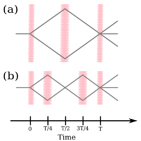
Figure 1: (color online) Trajectories of the BEC clouds as functions of time for (a) a single reflection interferometer and (b) a double reflection interferometer. Vertical wavy bands show timing of the optical pulses.

The first experiments using this type of interferometer were done by Wang et al. Wang et al. (2005). Good contrast of the interference fringes was observed for cycle times not exceeding about 10 ms. This fact was theoretically explained by Olshanii et al. Olshanii and Dunjko (2005). The authors of Ref.  Olshanii and Dunjko (2005) attributed the loss of contrast to a distortion of the phase across each harmonic that was caused by both the atom-atom interactions and the residual potential along the waveguide.

A simple way to understand the reason for the loss of contrast is to consider the effect of the two forces acting on the harmonics $\psi_{\pm}$ during the interferometric cycle. The first force is due to a repulsive nonlinearity between the two BEC clouds, as shown in Fig. 2 (a). This force exists only when the two harmonics overlap. The second force is exerted by the trapping potential along the waveguide and pushes the harmonics toward the center of the trap as shown in Fig. 2 (b). As a result, the velocities of the harmonics are not equal to their initial values $\pm v_{0}$ during the interferometric cycle.

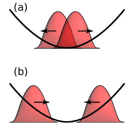
Figure 2: (color online) The two different forces acting on the two harmonics during the interferometric cycle. (a) When the two harmonics overlap, the atom-atom interactions cause a repulsive force between the harmonics and (b) the external potential exerts a force pushing the two harmonics towards the center of the trap.

Consider, for example, the $\psi_{+}$ harmonic. Just before the reflection pulse its velocity is $v_{0}+\delta v$. Since the reflection pulse changes the speed of each harmonic by $2v_{0}$, just after the reflection pulse the velocity of the $\psi_{+}$ harmonic becomes $-v_{0}+\delta v$. Because of this fact, when the harmonic moves back to the center of the trap, its velocity before the recombination is not equal to $-v_{0}$. The change in the speeds of the harmonics during the first and the second halves of the interferometric cycle has two consequences. First, harmonics do not completely overlap at the nominal recombination time. Second, the recombination optical pulse is unable to exactly cancel the harmonics’ velocities causing the recombined wave functions to have coordinate-dependent phases across the clouds. Both mechanisms result in a washout of interference fringes and loss of contrast.

A modification of the single-pass interferometer interferometer shown in Fig. 1 (b), was built by Garcia et al. Garcia et al. (2006). The interferometric cycle begins by illuminating the BEC with a splitting pulse. The two harmonics freely propagate until the time $t=T/4$ when they are illuminated by a reflection pulse. They continue to freely propagate until the time $t=3T/4$ when a second reflection pulse is applied. The harmonics freely propagate until the time $t=T$ when they overlap and are subject to the action of the recombination pulse. This type of an interferometer will be referred to as a double reflection interferometer. The coherence time demonstrated in Ref. Garcia et al. (2006) exceeded 44 ms. More recently, the coherence time of this interferometer has been extended to over 80 ms Burke et al. (2007). The advantage of a double reflection interferometer over a the single reflection one is in that the shift in the velocity of the harmonics is considerably reduced allowing for larger cycle times. Recently this type of interferometer was used to measure the ac Stark shift Deissler et al. (2007).

Along with the experimental realization of the single and double reflection interferometer, the authors of Ref. Burke et al. (2007) developed a theoretical model to describe its operation. The model presented in this paper differs from that of Ref. Burke et al. (2007) by accounting for the effects of atom-atom interactions, the change in the BEC size during the cycle time, and the incomplete overlap of the two harmonics at the recombination time. These effects do not significantly change the results of analysis of Ref. Burke et al. (2007) for the single reflection interferometer. However, our results for the double reflection interferometer are of a different functional form than those found in Ref. Burke et al. (2007).

In the rest of the paper, we use a simple analytic model to calculate the momentum and the degree of overlap of the two harmonics at the end of the cycle for both the single and double reflection interferometers. Both of these depend on the time that the two harmonics spend overlapping, the total cycle time and the frequency of the trap. Next, we find the regions of a large and a small interference fringe contrast for both the single and double reflection interferometers. We demonstrate that, with a double reflection interferometer, the coherence time can be increased by shifting the recombination time. Finally, we compare the model with recent experimental realizations of these interferometers.

II Analytical model

The dynamics of a BEC in a waveguide will be analyzed in the framework of the Gross-Pitaevskii equation (GPE)

$$i\frac{\partial}{\partial\tau}\psi(x,\tau)=\left[-\frac{1}{2}\frac{\partial^{2}}{\partial x^{2}}+v(x)+\Omega(\tau)\cos x+p|\psi|^{2}\right]\psi(x,\tau),$$ (1)

which has been obtained by projecting the three-dimensional GPE onto the strongly confining transverse mode of the waveguide (for more details see Stickney et al. (2007)). In Eq. (1), $\psi$ is the wave function of the BEC normalized to one, the dimensionless coordinate $x$ is measured in units of $x_{0}=1/2k_{l}$ and the dimensionless time $\tau$ is measured in units of $t_{0}=M/4\hbar k_{l}^{2}$, where $k_{l}$ is the wave vector of the lasers and $M$ is the atomic mass.

The weakly confining potential along the guide is harmonic

$$v(x)=\frac{1}{2}\omega^{2}x^{2},$$ (2)

and $\Omega(\tau)\cos x$ is the potential associated with the laser beams. The strength of interatomic interaction is given by the parameter

$$p=a_{s}N/a_{\perp}^{2}k_{l},$$ (3)

where $a_{s}$ is the s-wave scattering length, $N$ is the total number of atoms in the BEC, $a_{\perp}=\sqrt{\hbar/M\omega_{\perp}}$ is the transverse harmonic oscillator length, and $\omega_{\perp}$ is the transverse frequency of the guide.

The optical potential $\Omega(\tau)\cos x$ acts as a diffraction grating for the BEC wave function $\psi$. This grating diffracts the BEC into several harmonics separated by multiples of the grating wave vector:

$$\psi=\sum_{n}\psi_{n}e^{inx},$$ (4)

where $\psi_{n}$ are the slowly-varying amplitudes of the harmonics’ wave functions.

The dynamics of the BEC due to the optical potential has been discussed in Refs. Wu et al. (2005); Garcia et al. (2006); Stickney et al. (2007). Since the optical pulses used to manipulate the BEC are intense and short their action can be described by simple mixing matrices operating on the harmonics $\psi_{n}$ in Eq. (4). The splitting pulse transforms the initial zero-momentum harmonic $\psi_{0}$ into the two harmonics with $n=\pm 1$: $\psi_{0}\rightarrow(\psi_{+1}+\psi_{-1})/\sqrt{2}$. The reflection pulse transforms the $n=\pm 1$ harmonic into the $n=\mp 1$ harmonic: $\psi_{\pm 1}\rightarrow\psi_{\mp 1}$. Finally, after the recombination pulse, the BEC consists of three harmonics with $n=-1,0,+1$. The population in the zero momentum harmonic $\psi_{0}$ depends on the relative phase shift of the $\pm 1$ harmonics immediately before the recombination.

Between the splitting and the recombination optical pulses, the BEC consists of two harmonics with $n=\pm 1$. In the Thomas-Fermi approximation, the evolution of these harmonics is governed by the set of equations

$$\left(\frac{\partial}{\partial\tau}\pm\frac{\partial}{\partial x}\right)n_{\pm}=-\frac{\partial}{\partial x}\left(n_{\pm}\frac{\partial\phi_{\pm}}{\partial x}\right),$$

$$\left(\frac{\partial}{\partial\tau}\pm\frac{\partial}{\partial x}\right)\phi_{\pm}=-\frac{1}{2}\left(\frac{\partial\phi_{\pm}}{\partial x}\right)^{2}-v-p(n_{\pm}+2n_{\mp}),$$ (5)

where $n_{\pm}$ and $\phi_{\pm}$ are densities and phases of the harmonics introduced by the relations

$$\psi_{\pm 1}=\sqrt{n_{\pm}}\exp(i\phi_{\pm}).$$ (6)

Equations (II) are valid when $pR\gg 1$, where $p$ is the dimensionless nonlinearity parameter and $R$ is the characteristic size of the harmonics.

The set of partial differential equations Eqs. (II) can be transformed into a set of ordinary differential equations by parametrizing the density and phase of the harmonics as

$$n_{\pm} = \frac{3}{8R}\left[1-\frac{(x-x_{\pm})^{2}}{R^{2}}\right],$$

$$\phi_{\pm} = \varphi_{\pm}+\kappa_{\pm}(x-x_{\pm})+\frac{g}{2}(x-x_{\pm})^{2}+\frac{1}{6}s_{\pm}(x-x_{\pm})^{3}.$$ (7)

Functions $R$, $x_{\pm}$, $\varphi_{\pm}$, $\kappa_{\pm}$, $g$, and $s_{\pm}$ depend only on time. The radius of each of the harmonics is $R$. The position of each harmonics’s center of mass is given by the coordinate $x_{\pm}$. The coordinate-independent part of the phase of each harmonic is $\varphi_{\pm}$. The correction to the wave vector of each harmonic is $\kappa_{\pm}$ and the curvature of the phase is given by the parameter $g$. Finally, the parameter $s_{\pm}$ determines the size of the cubic contribution to the phase.

Using Eqs. (II) in Eqs. (II) results in a set of ordinary differential equations for the parameters $R$, $x_{\pm}$, $\varphi_{\pm}$, $\kappa_{\pm}$, $g$. These equations are

$$R^{\prime}=gR,$$

$$x_{\pm}^{\prime}=\pm 1+\kappa_{\pm},$$

$$\kappa_{\pm}^{\prime}=-\omega^{2}x_{\pm}\pm\frac{\omega^{2}R_{0}^{3}}{4R^{2}}d_{1}(q),$$

$$g^{\prime}=-g^{2}-\omega^{2}+\frac{\omega^{2}R_{0}^{3}}{2R^{3}}[1+d_{2}(q)],$$

$$s^{\prime}_{\pm}=\frac{6}{2}\frac{\omega^{2}R_{0}^{3}}{2R^{4}}d_{3}(q),$$

$$\varphi_{\pm}^{\prime}=\frac{1}{2}\kappa_{\pm}^{2}-\frac{1}{2}\omega^{2}x_{\pm}^{2}+\frac{\omega^{2}R_{0}^{3}}{4R}[1+d_{0}(q)].$$ (8)

Here

$$d_{0}=\left(2-\frac{7}{2}|q|^{2}+2|q|^{3}-\frac{1}{8}|q|^{5}\right)\theta(|q|<2),$$

$$d_{1}=q\left(4+\frac{15}{2}|q|-\frac{35}{2}|q|^{2}+\frac{65}{8}|q|^{3}-\frac{7}{16}|q|^{5}\right)\theta(|q|<2),$$

$$d_{2}=\left(2-\frac{15}{2}|q|^{2}+5|q|^{3}-\frac{3}{8}|q|^{5}\right)\theta(|q|<2),$$

$$d_{3}=q\left(-\frac{35}{2}|q|+\frac{175}{6}|q|^{2}-\frac{105}{8}|q|^{3}+\frac{35}{48}|q|^{5}\right)\theta(|q|<2),$$ (9)

and $q=(x_{+}-x_{-})/R$ is the relative displacement of the two harmonics. The $\theta$ function in Eq. (II) is equal to one if its argument is a logical true and zero if it is a logical false. The nonlinearity parameter $p$ was eliminated from Eqs. (II) with the help of the relation

$$p=\frac{2}{3}\omega^{2}R_{0}^{3},$$ (10)

where $R_{0}$ is the initial size of the BEC cloud (equal to the size of the both harmonics immediately after the splitting pulse). Equation (10) assumes that the BEC is created in the confining potential Eq. (2).

The procedure of deriving Eqs. (II) parallels that given in Stickney et al. (2007). Equations (II) and (II) differ from those found in Ref. Stickney et al. (2007) by accounting for an additional cubic term.

Since the BEC is in the lowest stationary state of the trap before the splitting pulse, the initial conditions for Eqs. (II) are $R(\tau=0)=R_{0}$, and $x_{\pm}(\tau=0)=\kappa_{\pm}(\tau=0)=g(\tau=0)=\varphi_{\pm}(\tau=0)=0$. The reflection pulses are accounted for by the boundary conditions at the time of the reflections: $x_{\pm}\rightarrow x_{\mp}$ and $\kappa_{\pm}\rightarrow\kappa_{\mp}$.

After the recombination pulse the BEC consists of three harmonics $\psi_{0}$ and $\psi_{\pm}$. The population of the zero-momentum harmonic is given by the expression

$${N_{0}}=\frac{1}{2}\left[1+V\cos\Delta\varphi\right],$$ (11)

where $\Delta\varphi=\varphi_{+}-\varphi_{-}$ is the relative phase difference between the harmonics.

The fringe contrast $V$ is given by the relation

$$V=\frac{3}{2}\int_{0}^{1-|\Delta x|/2R}dy\left[\left(1-y^{2}+\frac{(\Delta x)^{2}}{4R^{2}}\right)^{2}-\frac{(\Delta x)^{2}}{R^{2}}\right]^{1/2}\cos(\Delta kRy+\frac{1}{6}\Delta sR^{3}y^{3}).$$ (12)

Here

$$\Delta k=\Delta\kappa-g\Delta x+\frac{1}{8}\Delta s(\Delta x)^{2},$$ (13)

$\Delta x=x_{+}-x_{-}$, $\Delta\kappa=\kappa_{+}-\kappa_{-}$ and $\Delta s=s_{+}-s_{-}$.

When the fringe contrast is high ($1-V\ll 1$ ), Eq. (12) can be simplified to

$$V \approx 1-\frac{3}{2}\left(\frac{\Delta x}{2R}\right)^{2}\left[\ln\left|\frac{2R}{\Delta x}\right|+2\ln 2-\frac{1}{2}\right]$$ (14)

$$- \frac{1}{10}\left(\Delta kR+\frac{1}{14}\Delta sR^{3}\right)^{2}-\frac{1}{6615}(\Delta sR^{3})^{2}$$

$$= 1-A-B-C,$$

where $0\leq A,B,C\ll 1$.

The expression for the fringe contrast $V$ given by Eq. (14) contains three terms $A$, $B$, and $C$. All these terms are positive and decrease the fringe contrast additively. In the following analysis their influence will be considered separately. The boundary between the regions of high and low fringe contrast will be defined by the conditions $A\sim 1/2$, or $B\sim 1/2$, or $C\sim 1/2$. Despite the fact that Eq. (14) was obtained in the limit $A,B,C\ll 1$, these conditions turn out to be good qualitative and quantitative approximations.

The term

$$A=\frac{3}{2}\left(\frac{\Delta x}{2R}\right)^{2}\left[\ln\left|\frac{2R}{\Delta x}\right|+2\ln 2-\frac{1}{2}\right]$$ (15)

describes the decrease in the fringe contrast due to the incomplete overlap of the two harmonics at the recombination time. The region of low contrast due to the incomplete overlap is given by the condition

$$|\Delta x|/R\gtrsim 1$$ (16)

(the harmonics overlap by less than half of their their full widths).

The term

$$B=\frac{1}{10}\left(\Delta kR+\frac{1}{14}\Delta sR^{3}\right)^{2}$$ (17)

describes the loss of fringe contrast due to the phase difference between the center and the periphery of the cloud $\psi_{0}$. The region of low fringe contrast is given by the relation

$$\left|\Delta kR+\frac{1}{14}\Delta sR^{3}\right|\gtrsim\sqrt{5}\sim 2.$$ (18)

The phase difference in Eq. (17) is due to a combination of both the quadratic and the cubic terms in the expression for the phase (II). These terms have been grouped together in Eq. (17) because it is sometimes possible to set $B=0$ by shifting the recombination time, as will be shown in Sec. IV. However, even when $B=0$, there are higher order phase distortions that can cause a loss of fringe contrast due to the presence of the cubic term in the phase Eq. (II). The effect of this cubic term on the fringe contrast is given by the parameter

$$C=\frac{1}{6615}(\Delta sR^{3})^{2}.$$ (19)

This term results in a small fringe contrast when

$$\left|\Delta s\right|R^{3}\gtrsim\sqrt{6615/2}\sim 60.$$ (20)

Each of the three above-discussed contributions to the Eq. (14) can be expressed in terms of three dimensionless parameters having a simple physical meaning. The first parameter is the dimensionless trapping frequency

$$\omega=\omega_{\parallel}t_{0},$$ (21)

The second parameter is the product of the interferometric cycle time and the trapping frequency

$$\omega T=\omega_{\parallel}T_{D}$$ (22)

where $\omega_{\\ }$ and $T_{D}$ are the dimensional trap frequency and the cycle time, respectively.

The third parameter is the product of the dimensionless initial size of the BEC $R$ and the trapping frequency $\omega$. This parameter can be written in terms of dimensional quantities as

$$\omega R=\frac{\omega_{\parallel}R_{D}}{v_{0}},$$ (23)

where $R_{D}$ is the dimensional radius of the BEC and $v_{0}=2\hbar k_{l}/M$ is the speed of the harmonics just after the splitting pulses. This parameter is the time it takes the two harmonics to separate measured in units of the inverse trapping frequency.

III Single reflection interferometer

Solutions of Eqs. (II) for the case of a single reflection interferometer shown in Fig. 1 (a) have been previously discussed in Stickney et al. (2007) without the cubic phase term. Inclusion of this term ($\Delta s$) is somewhat cumbersome but straightforward and results in the following expressions for $R$, $\Delta x$, $\Delta\kappa$, $g$ and $\Delta s$ at the end of the interferometric cycle of duration $T$:

$$R = R_{0}[1-\frac{1}{4}(\omega T)^{2}],$$

$$\Delta x = \frac{1}{4\omega}(\omega T)^{3},$$

$$\Delta\kappa = \frac{1}{2}(\omega T)^{2}-2(\omega R_{0})^{2}D_{1}(\omega T/\omega R_{0}),$$

$$g = -\omega[\omega T-2\omega R_{0}D_{2}(\omega T/\omega R_{0})],$$

$$\Delta s = 2\omega^{2}D_{3}(\omega T/\omega R_{0}).$$ (24)

Here

$$D_{1}(x)=\left\{\begin{array}[]{ccc}\frac{1}{4}x^{2}(2+\frac{5}{2}x-\frac{35}{8}x^{2}+\frac{13}{8}x^{3}-\frac{1}{16}x^{5})&,&x<2\\ 1/2&,&x>2\end{array}\right.,$$ (25)

$$D_{2}(x)=\left\{\begin{array}[]{ccc}\frac{1}{4}x\left(2-\frac{5}{2}x^{2}+\frac{5}{4}x^{3}-\frac{1}{16}x^{5}\right)&,&x<2,\\ 0&,&x>2.\end{array}\right.,$$ (26)

and

$$D_{3}(x)=\left\{\begin{array}[]{ccc}\frac{3}{2}x^{3}\left(\frac{35}{6}-\frac{175}{24}x+\frac{21}{8}x^{2}-\frac{5}{48}x^{4}\right)&,&x<2,\\ 1&,&x>2.\end{array}\right.$$ (27)

In deriving the above expressions, only the lowest order contributions in terms of $\omega T$ and $\omega R$ were retained. The loss of the fringe contrast takes place when both these parameters are still small. The first of Eq. (24) then shows that the relative change in the size of the BEC during the cycle is small and will be neglected in the subsequent analysis.

The loss of the contrast due to the term $A$ Eq. (15) happens for $A>1/2$. Using Eqs. (16) and (24), we can translate this inequality into the relation

$$\frac{1}{4}\frac{(\omega T)^{3}}{\omega R}>1.$$ (28)

Similarly, the loss of the contrast due to the term $B$ Eq. (17) with the help of Eqs. (18) and (24) can be expressed as

$$\left\{\frac{1}{2}(\omega T)^{2}-2(\omega R)^{2}\left[D_{1}(\omega T/\omega R)-\frac{1}{14}D_{3}(\omega T/\omega R)\right]\right\}\frac{\omega R}{\omega}>5,$$ (29)

where $D_{1}$ and $D_{3}$ are given by Eqs. (25) and (27) respectively.

Finally, the loss of the fringe contrast due to the term $C$ corresponds to the region of parameters where

$$\frac{(\omega R)^{3}}{\omega}D_{3}(\omega T/\omega R)>30.$$ (30)

Figure 3 is a two-dimensional plot showing the regions of operation of the interferometer. The dimensionless trap frequency is $\omega=3.5\times 10^{-5}$, which roughly corresponds to the value used in recent experiments Burke et al. (2007). The white region corresponds to large fringe contrast. In the grey region (lower right corner) $A>1/2$ and the fringe contrast is small because of the lack of overlap of the harmonics $\psi_{\pm}$. The region with the vertical stripes corresponds to $B>1/2$ and the contrast is small because of the phase difference across the cloud. The region filled with the horizontal stripes corresponds to $C>1/2$ and the contrast is lost because of large value of the cubic phase across the harmonic. These regions were found by numerically inverting Eqs. (28), (29), and (30). Note that when two shaded regions overlap, the contrast is lost due to two different mechanisms.

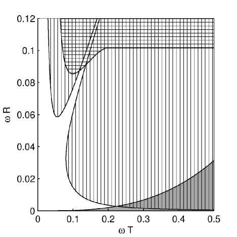
Figure 3: The regions of large and small fringe contrast for the single reflection interferometer. The white region corresponds to high contrast. In the grey region $A>1/2$, the region filled with vertical stripes is where $B>1/2$. The region filled with horizontal stripes is where $C>1/2$.

Figure 3 shows that when $\omega R<5\times 10^{-3}$, the contrast is lost because the two harmonics $\psi_{\pm}$ do not overlap at the recombination time. In the region $5\times 10^{-3}<\omega R<6\times 10^{-2}$, the contrast is lost because the trap causes a difference in the phase across the atomic cloud. When $\omega R>6\times 10^{-3}$ and $\omega T<\sqrt{2}\omega R$, the force that the two harmonics exert on each other is the cause of the difference in phase across the harmonics. For the cycle time $\omega T=\sqrt{2}\omega R$, there is no phase difference across the harmonics, but for $\omega T>0.12$ the cubic phase across the recombined harmonic causes a loss of fringe contrast. For $\omega R>0.06$ and $\omega T>\sqrt{2}\omega R$ the trap causes the loss of fringe contrast.

The boundary between the regions where $A<1/2$ and $A>1/2$ is given by the relation

$$\omega R=\frac{1}{4}(\omega T)^{3}.$$ (31)

For a given value of $\omega T$, Eq. (31) sets the lower limit on the parameter $\omega R$ for which the fringe contrast is large.

The boundary between the regions where $B<1/2$ and $B>1/2$ obtained with the help of Eq. (18) in the limit $\omega R\ll 1$, is given by the relation

$$\omega R=\frac{4\omega}{(\omega T)^{2}}.$$ (32)

For a given $\omega T$, Eq. (32) is the upper limit on the parameter $\omega R$ for which the fringe contrast is large.

The largest cycle times with high fringe contrast correspond to the point on Fig. 3 where the grey and vertical striped regions meet. Eqs. (31) and (32) show that the maximum cycle time is given by

$$\omega T_{max}=(16\omega)^{1/5}$$ (33)

and this occurs when the size of the BEC is given by the relation

$$\omega R_{opt}=\frac{1}{4}(16\omega)^{3/5}.$$ (34)

The optimal value of the parameter $\omega R_{opt}$ is always smaller than $\omega T_{max}$, which justifies the approximation used in deriving Eq. (32).

In a previous paper Stickney et al. (2007), we demonstrated that it is sometimes possible to increase the contrast of the interference fringes by shifting the recombination time. However, in the geometry of a single-reflection interferometer when the BEC is created in the confining potential given by Eq. (2), it is not possible to significantly increase the fringe contrast by shifting the recombination time for $\omega T/\omega R>2$, i.e., for the cycle times such that the two clouds completely separate. As a result, the regions depicted in Fig. 3 cannot be significantly changed by shifting the recombination time.

IV Double reflection interferometer

For the geometry of the double reflection interferometer shown in Fig.1 (b), expressions for $R$ and $g$ were found by perturbatively solving Eqs. (II) to third order in $\omega T$ and first order in $\omega R$ yielding

$$g = \omega\left[-\frac{1}{2}(\omega T)+\frac{1}{24}(\omega T)^{3}+\frac{1}{4}(\omega R)D_{2}\left(\frac{\Delta x}{R}\right)\right],$$

$$R = R_{0}\left[1-\frac{1}{4}(\omega T)^{2}\right].$$ (35)

The equation for $R$ shows that, as for the single reflection interferometer, the relative change in the size of the BEC during the cycle is small. This change will be neglected in the subsequent analysis.

Solutions of Eqs. (II) results in the expressions for $\Delta x$ and $\Delta\kappa$ at the end of the interferometric cycle that are given by

$$\Delta x = \frac{2}{\omega}\left[2\sin\frac{\omega T}{4}-2\sin\frac{3\omega T}{4}+(1+I_{s})\sin\omega T\right],$$

$$\Delta\kappa = 4\cos\frac{\omega T}{4}-4\cos\frac{3\omega T}{4}+2(1+I_{s})\cos\omega T-2+2I_{r}.$$ (36)

Here

$$I_{s}=\frac{1}{4}(\omega R)^{2}$$ (37)

is the change in $\Delta\kappa$ caused by the repulsive force that the two harmonics exert on each other during the separation and

$$I_{r}=\frac{1}{2}(\omega R)^{2}\left[D_{1}(|\Delta x|/R)-\frac{1}{2}\right]\approx-\frac{1}{4}(\omega R)^{2}\left[1-\left(\frac{\Delta x}{R}\right)^{2}\right]$$ (38)

is the change in $\Delta\kappa$ caused by the force that the two harmonics exert on each other during the recombination, with $D_{1}$ given by Eq. (25). Expanding Eq. (36) into into a Taylor series and keeping up to the sixth order in $\omega T$ results in the relations

$$\Delta x = \frac{2}{\omega}\left[\frac{1}{4}(\omega R)^{2}(\omega T)-\frac{1}{32}(\omega T)^{3}+\frac{9}{2048}(\omega T)^{5}\right],$$

$$\Delta\kappa = \frac{1}{2}(\omega R)^{2}\left[\left(\frac{\Delta x}{R}\right)^{2}-\frac{1}{2}(\omega T)^{2}\right]+\frac{1}{32}(\omega T)^{4}-\frac{11}{6144}(\omega T)^{6}.$$ (39)

The first term in Eq. (38) is canceled by Eq. (37) and the incomplete overlap at the recombination time has a larger effect than the change in the harmonics’ size $R$.

Finally, $\Delta s$ is given by the expression

$$\Delta s=-\omega^{2}\left[1+\left(\frac{R_{0}}{R}\right)^{3}\left(D_{3}(|\Delta x|/R)-1\right)\right],$$ (40)

where $D_{3}$ is given by Eq. (27). Here, the change in the size of the harmonics $R$ has a larger effect on $\Delta s$ than the incomplete overlap at the recombination time. In the limit where the change in $R$ is small and using Eq. (35), reduces Eq. (40) to

$$\Delta s=-\omega^{2}\frac{3}{4}(\omega T)^{2}.$$ (41)

The loss of contrast due to the term $A$ Eq. (15) occurs when $A>1/2$. Using Eq. (16) and (39), we can translate this inequality into the relation

$$\frac{1}{16}\frac{(\omega T)^{3}}{\omega R}>1.$$ (42)

Similarly, the loss of contrast due to B Eq. (17) is given by Eq. (18) and Eq. (13), which is the sum of three terms. The first term is

$$\Delta\kappa=\frac{1}{32}(\omega T)^{4}+\frac{1}{6144}(\omega T)^{6}-\frac{3}{8}(\omega R)^{2}(\omega T)^{2}.$$ (43)

The second term is the product of the distance between the two harmonics and the quadratic contribution to the phase at the recombination time and may be expressed as

$$g\Delta x=\frac{1}{32}(\omega T)^{4}-\frac{9}{2048}(\omega T)^{6}-\frac{1}{4}(\omega R)^{2}(\omega T)^{2}.$$ (44)

The third term is the cubic contribution given by

$$\Delta sR^{3}=\frac{3}{4\omega}(\omega T)^{2}(\omega R)^{3}.$$ (45)

Adding Eq. (43), (44), and (45), the inequality $B>1/2$ can be translated into the relation

$$\left|\frac{1}{192}(\omega T)^{6}-\frac{1}{14}(\omega R)^{2}(\omega T)^{2}\right|\frac{\omega R}{\omega}>2.$$ (46)

The region were the loss of contrast is caused by C can be found using Eqs. (45) and (20) and results in the relation

$$\frac{1}{\omega}(\omega T)^{2}(\omega R)^{3}>80.$$ (47)

Figure 4 is a two dimensional plot showing the regions of operation of a double reflection interferometer. The dimensionless trap frequency is $\omega=3.5\times 10^{-5}$ as in Fig. 3. The white region corresponds to large contrast. In the grey region (lower right corner) $A>1/2$ and the contrast is small due to incomplete overlap at the recombination time. The region filled with vertical stripes corresponds to $B>1/2$ and the contrast is small due to the phase difference across the recombined BEC. The region filled with horizontal stripes corresponds to $C>1/2$ and the cubic phase causes the loss of contrast.

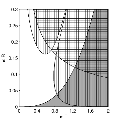
Figure 4: The regions of large and small fringe contrast for the double reflection interferometer. The white region corresponds to large contrast. In the grey region $A>1/2$. The region filled with vertical stripes is where $B>1/2$. The region filled with horizontal stripes is where $C>1/2$.

For $\omega R<0.04$, the contrast is lost because the two harmonics $\psi_{\pm}$ do not overlap at the recombination time. In the region $0.04<\omega R$ the contrast is lost because the trap causes a phase difference across the recombined harmonic. Along the curve $\omega R=\sqrt{7/96}(\omega T)^{2}$ the phase difference across the recombined harmonic vanishes and $B=0$. However, when $\omega T>0.8$, the cubic phase causes the loss of contrast and $C>1/2$.

When the contrast is lost because of the incomplete overlap of the clouds at the nominal recombination time (term $A$, grey region in Fig 4), the contrast can be increased by recombining when the two clouds overlap. Using Eqs. (II) and (42), it can be shown that the two harmonics completely overlap at the time $\tau=T+\Delta T$, where

$$\frac{\Delta T}{R}=\frac{1}{16}\frac{(\omega T)^{3}}{\omega R}.$$ (48)

At this shifted time, the contrast still may be lost due to the term $B$ if

$$\left|\frac{1}{32}(\omega T)^{4}-\frac{1}{28}(\omega R)^{2}(\omega T)^{2}\right|\frac{\omega R}{\omega}>1$$

and due to $C$ if Eq. (47) is fulfilled. This method for increasing the contrast is only useful when $\omega R<(\omega^{3}/2)^{1/7}$.

Figure 5 is a two-dimensional plot showing the regions of operation when the recombination pulse is applied at the time when the two clouds overlap. The dimensionless trap frequency is $3.5\times 10^{-5}$. The white region corresponds to large values of the fringe contrast. The region filled with vertical stripes corresponds to $B>1/2$ and the region filled with horizontal stripes to $C>1/2$. Recombination at a shifted time improves the fringe contrast for $\omega R<0.01$.

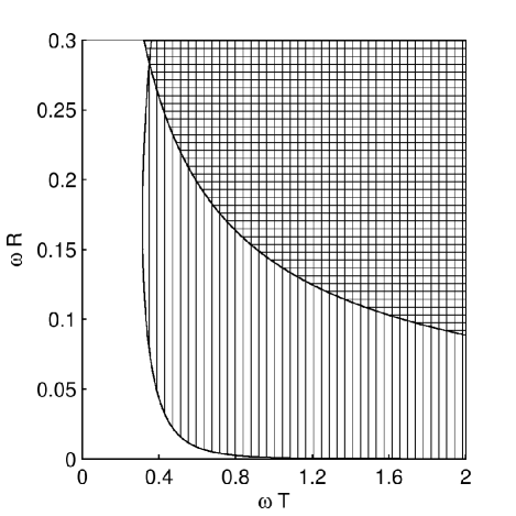
Figure 5: The regions of large and small fringe contrast for the double reflection interferometer. The recombination takes place at the time, when the harmonics fully overlap and $A=0$. The white region corresponds to large contrast. The region filled with vertical stripes is where $B>1/2$ and the region filled with horizontal stripes is where $C>1/2$.

When the contrast is lost because of the term $B$ (vertical stripes in Fig. 4), the contrast also can be increased by shifting the recombination time. This is because the quantity that determines the contrast in Eq. (18) is the sum of the three terms given by Eqs. (43), (44), and (45). A small change in the recombination time results in a change in Eq. (44), but does not change either Eq. (43) or Eq. (45). Using Eqs. (II) one can show that recombining at the time $\tau=T+\Delta T$, where

$$\frac{\Delta T}{R}=\frac{1}{192}\frac{(\omega T)^{5}}{\omega R}-\frac{1}{14}(\omega T)(\omega R),$$ (49)

results in $B=0$ at the shifted recombination time. With the help of Eqs. (II), (46) and (49), the inequality $A>1/2$ at the shifted recombination time translates into the relation

$$\frac{\Delta\kappa}{gR}=\frac{1}{16}\frac{(\omega T)^{3}}{\omega R_{0}}>1,$$ (50)

The region where $C>1/2$ is still given by Eq. (47). Figure 6 is a two-dimensional plot showing the different regions of operation when the recombination takes place at the shifted time given by Eq. (49). The dimensionless trap frequency is taken to be $\omega=3.5\times 10^{-5}$. The white region corresponds to large values of the fringe contrast. In the grey region the loss of contrast is caused by the term $A$ and in the region filled with horizontal stripes by the term $C$.

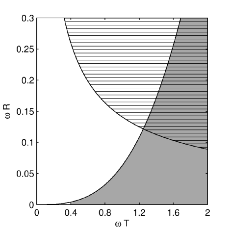
Figure 6: The regions of large and small fringe contrast for the double reflection interferometer, when the recombination takes place at the optimal time, when $B=0$. The white region corresponds to large values of the contrast. In the grey region $A>1/2$ and in the region filled with horizontal stripes $C>1/2$.

When $\omega R<0.13$, the incomplete overlap causes the loss of fringe contrast and when $\omega R>0.13$ the cubic phase causes the loss of contrast.

The lower limit on the values of $\omega R$ for which the fringe contrast is large with the help of Eq. (50) can be written as

$$\omega R\approx\frac{1}{16}(\omega T)^{3}.$$ (51)

and the upper limit on $\omega R$ using Eq. (47) can be expressed as

$$\omega R=\frac{(30\omega)^{1/3}}{(\omega T)^{2/3}}.$$ (52)

The longest cycle time before the loss of the fringe contrast is given by the relation

$$\omega T_{max}\approx 3\omega^{1/11},$$ (53)

and occurs when the size of the BEC is

$$\omega R_{opt}\approx\frac{27}{16}\omega^{3/11}.$$ (54)

V Comparison with experiment

There have been several experimental realizations of waveguide interferometers that use optical pulses to control the dynamics of the BEC Wang et al. (2005); Horikoshi and Nakagawa (2006); Garcia et al. (2006); Burke et al. (2007); Deissler et al. (2007).

The JILA group Wang et al. (2005) built a single reflection interferometer and used a trap with frequencies $(\omega_{x},\omega_{y},\omega_{z})=2\pi\times(100,100,5)$ Hz and a ${}^{87}\mbox{Rb}$ BEC with about $10^{4}$ atoms. These parameters correspond to the nonlinearity parameter $p=5.7$, the dimensionless BEC radius $R=675$, the dimensionless trap frequency of $\omega=1.7\times 10^{-4}$ and $\omega R=0.11$. In Ref. Wang et al. (2005) the contrast at about 10 ms was found to be $V=0.2$. This agrees with our model if, instead of using Eqs. (24) and Eq. (14), we use Eq. (24) and numerically integrate Eq. (12).

In the experiment at the University of Virginia Burke et al. (2007) the trap has frequencies $(\omega_{x},\omega_{y},\omega_{z})=2\pi\times(3.3,6,1.2)$ Hz, and the BEC had about $3\times 10^{4}$ ${}^{87}\mbox{Rb}$ atoms. These parameters correspond to the dimensionless nonlinearity parameter $p\approx 0.75$, the dimensionless BEC radius of $R=940$, the dimensionless trap frequency of $\omega=3.65\times 10^{-5}$ and $\omega R=0.035$.

The University of Virginia group experimentally investigated the operation of both a single and double reflection interferometer. When analyzing the single reflection interferometer, they found 50% contrast for the cycle time of about 12 ms. This time corresponds to $\omega T=0.9$ (cf. Eq.(22)). The loss of contrast at this time agrees with Fig. 3 and the results of Sec. III.

The double reflection interferometer had 50% contrast for a cycle time of 80 ms, translating to $\omega T=0.6$ in our variables. The loss of contrast at this time agrees with Fig. 4 and the results of Sec. IV. The experiment used a BEC radius $R$ such that the contrast was lost due to both the incomplete overlap (term $A$) and the phase across the cloud (term $B$) at about the same cycle time $\omega T$. This may explains why the University of Virginia experiment had no phase distortion across the recombined BEC. An increase of decrease in the radius $R$ would have caused a decrease in the coherence time of the interferometer. However, our model predicts that by both increasing the radius and shifting the recombination time it would be possible to increase the coherence time.

VI Conclusions

In this paper, we analyzed the operation of both single and double reflection interferometers. We introduced a simple analytic model to determine the regions in parameter space where the fringe contrast is large and small. For the case of a double reflection interferometer, we showed that the coherence time can be increased by changing the recombination time. Finally, we compared our results to recent experimental realizations of these interferometers.

Our analysis focused on the case where the BEC was in the ground state of the trap at the beginning of the interferometric cycle. Analysis of the single reflection interferometer when this restriction is relaxed can be found in Stickney et al. (2007). In the case of a double reflection interferometer, the two largest terms (of order $(\omega T)^{4}$) in Eqs. (43) and (44) are only equal when the BEC is initially in the ground state. As a result, the region of high contrast discussed in Sec. IV becomes smaller when the BEC is not initially in the ground state.

The analysis of this paper did not include effects beyond the mean field approximation such as phase diffusion and finite temperature phase fluctuations.

The phase fluctuations of a BEC in a trap have been extensively studied in Ref. Lewenstein and You (1996); Javanaien and Wilkens (1997); Leggett and Sols (1998); Javanainen and Wilkens (1998). It has been shown that the phase diffusion time has the functional form $T_{D}\sim(\bar{a}_{HO}/a_{s})^{2/5}N^{1/10}/{\bar{\omega}}$ Javanaien and Wilkens (1997), where $\bar{\omega}=(\omega_{x}\omega_{y}\omega_{z})^{1/3}$ is the geometric average of the trap frequencies and $\bar{a}_{HO}=\sqrt{\hbar/M\bar{\omega}}$ is the average oscillator length. For the case of the University of Virginia experiment Burke et al. (2007), the phase diffusion time is $T_{D}\sim 3~{}\mbox{sec}$, which is much longer than the upper limit calculated in Sec. V.

When the aspect ratio of the trap $\omega_{\parallel}/\omega_{\perp}$ becomes sufficiently large, the BEC becomes one-dimensional and phase fluctuations can cause decoherence Petrov et al. (2001); Dettmer et al. (2001); Burkov et al. (2007); Hofferberth et al. (2007). The phase fluctuations along the BEC depend on the aspect ratio and temperature of the BEC and become important when the temperature of the BEC is larger than $T=15(\hbar\omega_{\parallel})^{2}N/32\mu$ Petrov et al. (2001), where $\mu$ is the chemical potential of the BEC. For the recent experiments Wang et al. (2005); Garcia et al. (2006), the phase fluctuations across the BEC are sufficiently small that they can be neglected.

VII Acknowledgements

This work was supported by the Defense Advanced Research Projects Agency (Grant No. W911NF-04-1-0043) and the National Science Foundation (Grant No. PHY-0551010).

References

- Wang et al. (2005) Y. Wang, D. Anderson, V. Bright, E. Cornell, Q. Diot, T. Kishimoto, M. Prentiss, R. Saravanan, S. Segal, and S. Wu, Phys. Rev. Letts. 94, 090405 (2005).
- Garcia et al. (2006) O. Garcia, B. Deissler, K. J. Hughes, J. M. Reeves, and C. A. Sackett, Phys. Rev. A 74, 031601 (2006).
- Wu et al. (2005) S. Wu, Y. Wang, Q. Diot, and M. Prentiss, Phys. Rev. A. 71, 043602 (2005).
- Olshanii and Dunjko (2005) M. Olshanii and V. Dunjko, arXiv.org:cond-mat/0505358 (2005).
- Burke et al. (2007) J. H. T. Burke, B. Deissler, K. J. Hughes, and C. A. Sackett, arXiv:0705.1081v1 (2007).
- Deissler et al. (2007) B. Deissler, K. J. Hughes, J. H. T. Burke, and C. A. Sackett, arXiv:0709.4675v1 (2007).
- Stickney et al. (2007) J. A. Stickney, D. Z. Anderson, and A. A. Zozulya, Phys. Rev. A. 75, 063603 (2007).
- Horikoshi and Nakagawa (2006) M. Horikoshi and K. Nakagawa, Phys. Rev. A. p. 031602 (2006).
- Wang (2005) Y.-J. Wang, Ph.D. thesis, University of Colorado (2005).
- Lewenstein and You (1996) M. Lewenstein and L. You, Phys. Rev. Letts. 77, 3489 (1996).
- Javanaien and Wilkens (1997) J. Javanaien and M. Wilkens, Phys. Rev. Letts. 78, 4675 (1997).
- Leggett and Sols (1998) A. Leggett and F. Sols, Phys. Rev. Letts. 81, 1344 (1998).
- Javanainen and Wilkens (1998) J. Javanainen and M. Wilkens, Phys. Rev. Letts. 81, 1345 (1998).
- Petrov et al. (2001) D. Petrov, G. Shlyapnikov, and J. Walraven, Phys. Rev. Letts. 87, 050404 (2001).
- Dettmer et al. (2001) S. Dettmer, D. Hellweg, P. Ryty, J. Arlt, W. Ertmer, K. Sengstock, D. Petrov, G. Shyapnikov, H. Kreutzmann, L. Santos, et al., Phys. Rev. Letts. 87, 160406 (2001).
- Burkov et al. (2007) A. Burkov, M. Lukin, and E. Demler, Phys. Rev. Letts. 98, 200404 (2007).
- Hofferberth et al. (2007) S. Hofferberth, I. Lesanovsky, B. Fischer, T. Schumm, and J. Schmiedmayer, arXiv.org:cond-mat/0706.2259v1 (2007).