Distributed Fair Scheduling Using Variable Transmission Lengths in Carrier-Sensing-based Wireless Networks

Abstract

The fairness of IEEE 802.11 wireless networks (including Wireless LAN and Ad-hoc networks) is hard to predict and control because of the randomness and complexity of the MAC contentions and dynamics. Moreover, asymmetric channel conditions such as those caused by capture and channel errors often lead to severe unfairness among stations. In this paper we propose a novel distributed scheduling algorithm that we call VLS, for “variable-length scheduling”, that provides weighted fairness to all stations despite the imperfections of the MAC layer and physical channels. Distinct features of VLS include the use of variable transmission lengths based on distributed observations, compatibility with 802.11’s contention window algorithm, opportunistic scheduling to achieve high throughput in time-varying wireless environments, and flexibility and ease of implementation. Also, VLS makes the throughput of each station more smooth, which is appealing to real-time applications such as video and voice. Although the paper mostly assumes 802.11 protocol, the idea generally applies to wireless networks based on CSMA (Carrier Sensing Multiple Access).

I INTRODUCTION

In this paper, we propose a simple distributed scheduling algorithm that provides weighted fairness in IEEE 802.11 [1] wireless networks, despite the unpredictability of the 802.11 MAC layer and physical channels.

In 802.11 wireless networks, MAC-layer contention, dynamics and bandwidth allocation are hard to predict. For such networks, the fixed-point model in [4] gives a method for computing the long-term throughput of the Binary Exponential Backoff (BEB) algorithm [1]. However, the short-term dynamics and unfairness are quite unpredictable. In a certain period, a station may randomly backoff more than others, and therefore have a smaller chance of winning the channel, which in turn makes that station backoff even more.

Meanwhile, the BEB amplifies the unfairness caused by the impairments of the wireless channels. This aggravation is an unintentional side effect of BEB that was designed to reduce collisions, not to guarantee fairness. The following two effects cause the unfairness:

• Capture: Capture occurs when the signals from different transmitters have very different strengths at a receiver [8]. For instance, a ratio of 2 in distances from the stations to the AP can lead to approximately a ratio of 16 in received signal strengths. When more than one station transmit packets to the AP at the same time, the AP may be able to capture and correctly decode the packet from the closer station, while ignoring the other packets. This effect increases the aggregate throughput since the AP receives one packet even when multiple transmissions overlap in time. However, capture may result in unfairness since the stations that are further away backoff more with the BEB algorithm, and consequently obtain much less throughput than closer stations [7].

• Channel errors: In addition to packet collisions, channel errors are another important cause of packet loss. A more lossy channel to the AP drops more packets because of channel errors. The transmitting station interprets all packet losses as collisions and doubles its contention window. Accordingly, the BEB algorithm magnifies the asymmetry of the lossy channels. To alleviate this problem, reference [11] describes a way to differentiate the two kinds of packet losses (due to collisions or channel errors). The algorithm proposed in this paper provides a simpler solution.

With a more complicated MAC, IEEE 802.11e [2] provides Differentiated Service (DiffServ), by adopting different minimum Contention Windows ($CW_{min}$) and inter-frame Spaces (IFS) for different service classes such as voice, video and data. This protocol provides relative performance differentiation among different classes: the classes with smaller $CW_{min}$ and IFS have a relative priority over others. To evaluate the performance of 802.11e, reference [14] provides a simulation study; while reference [13] uses an analytical model (a Markov chain) to find the saturated throughput of 802.11e. However, the model there is quite complicated, indicating that the “amount” of relative priority is hard to quantify and control. For instance, it is not clear how much more bandwidth the protocol gives to video with a particular setting of $CW_{min}$ and IFS, nor how to adjust the amount of priority by varying these parameters.

In this paper, we describe a simple, easy to implement, distributed fair scheduling algorithm that we call VLS, for“variable-length scheduling,” to cope with the above problems. VLS provides exact weighted fairness despite the unpredictability of the 802.11 MAC layer and physical channels.

II Variable-Length Scheduling (VLS): Bringing Order To Random Access

In this section, we assume that there is only one collision domain. That is, each station can sense the transmissions of other stations. (We consider the case of multiple collision domains in section V.) There are two versions of the scheduling algorithm: without and with an access point (AP). The latter is an adaptation of the former that utilizes the AP to simplify the algorithm.

II-A Distributed algorithm

The algorithm is based on the concept of “virtual slot.” By definition, a station sees a virtual slot when it senses a collision, a burst of transmissions (i.e., one DATA-ACK exchange, or a series of DATA-ACK exchanges separated by SIFS), or when it transmits a burst of packets itself. Mini-slots are not counted as virtual slots. In other words, a station counts a virtual slot whenever if senses the channel as “idle” for an interval equal to DIFS (DIFS$>$SIFS [1]) and is involved in a contention process (i.e., when the station’s backoff counter goes down until it transmits a packet or senses other transmissions). In Fig. 1, for example, there are 3 virtual slots. “Virtual slots” are similar to “busy slots” except that a burst of transmissions is counted as one “virtual slot.”

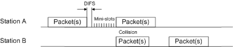
Figure 1: Virtual slots. (There are 3 virtual slots in this figure.)

The notion of “virtual slot” is particularly useful because every station in a single collision domain sees the same number of virtual slots, assuming that the stations are always backlogged. (If not, the station starts the algorithm only when it has a backlog and stops it when its backlog is cleared.) Therefore, virtual slots can serve as a “clock” for scheduling. We design the distributed algorithm as follows.

• Each station $j$ is assigned a “weight” $W_{j}$ [15]. (If there are multiple flows outgoing from station $j$, then let $W_{j}$ be the sum of the weights of all individual flows.) And each station $j$ keeps track of a value $m_{j}$ that is initially equal to 1.

• If station $j$ gets an ACK after it transmits a packet, it keeps transmitting a burst of $m_{j}W_{j}$ packets separated by SIFS and then resets $m_{j}$ to the value 1.

• If it does not get an ACK after it transmits a packet, or if it does not get to transmit (i.e., it does not win a contention), station $j$ increments $m_{j}$ by one whenever it sees a virtual slot.

For example, Fig. 2 shows the process with 2 stations with weights $w_{1}$ and $w_{2}$ respectively. In the figure, each block represents a virtual slot (aligned across different stations). The number in each block indicates the transmission length in that virtual slot. (Note that the size of a block here does not reflect the actual length of the virtual slot.) Assume station 1 starts transmission with the 1st virtual slot, while station 2 starts transmission with the 2nd.

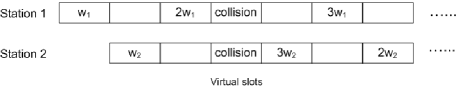
Figure 2: Variable-length Scheduling. ($w_{1}$, $w_{2}$ are the weights. Each block represents a variable-length virtual slot. The number in a block indicates the transmission length.)

In a time period when station $j$ is backlogged, we can see that the total number of packets it has transmitted is equal to the number of virtual slots it has seen so far times the weight $W_{j}$. (So station $j$ virtually transmits $W_{j}$ packets per slot. This is why we use the name “virtual slot”.) Since all stations see the same virtual slots, the bandwidth allocation is weighted fair. That is $T_{j}/W_{j}$ is the same for all the stations where $T_{j}$ is the average rate of packets that station $j$ transmits.

Note that VLS guarantees the weighted fairness, no matter what happens in the MAC and physical layers. Thus, VLS automatically adjusts for the randomness of the MAC protocol and the asymmetry of the physical channels.

II-B Algorithm with an AP

In a wireless LAN with an AP, the above algorithm can be adapted so that the client stations need not count the virtual slots. In this variation, the AP counts the virtual slots for the stations and piggybacks that count in the MAC-layer ACKs to the stations. The algorithm works as follows.

• The AP keeps counting the virtual slots. It increments the count ($v++$) for each virtual slot.

• A station can start and stop the algorithm at any time. When station $j$ starts, it contends for the channel and sends the first $W_{j}$ packets to the AP. In one ACK, the AP piggybacks the current value of $v$, denoted as $v_{i}^{j}$. The next time station $j$ wins the channel, it sends $W_{j}$ packets first. The AP, again, piggybacks the current value of $v$, denoted as $v_{i+1}^{j}$. Then, the station sends $W_{j}(v_{i+1}^{j}-v_{i}^{j}-1)$ more packets in the burst. Since $v_{i+1}^{j}-v_{i}^{j}-1\geq 0$, station $j$ sends at least $W_{j}$ packets per burst.

II-C Considerations on Burst Length

Suppose that, at each virtual slot, every station $i$ has a probability $p_{i}$ of winning the channel. Then on average, station $i$ accumulates $W_{i}/p_{i}$ units of “credit” before it wins the channel (since the average number of virtual slots it waits for is $1/p_{i}$). It can then spent the credits by transmitting (on average) $W_{i}/p_{i}$ packets. When the number of active stations $N$ increases in a wireless networks, $p_{i}$ decreases (approximately $\propto 1/N$). As a result, the average burst length increases, thus causing more delays for all the stations.

To avoid this effect, we define a system-wide parameter $c>0$, called “speed of the clock”, and we modify the protocol as follows:

• Instead of transmitting $m_{j}W_{j}$ packets in a burst as in subsection II-A, station $j$ transmits $c\cdot m_{j}W_{j}$ packets. If $c\cdot m_{j}W_{j}$ is not an integer, then it transmits $\left\lfloor c\cdot m_{j}W_{j}\right\rfloor$ packets, and saves the extra credits $c\cdot m_{j}W_{j}-\left\lfloor c\cdot m_{j}W_{j}\right\rfloor$ for the next time. Essentially, $c$ controls the speed of clock in the whole network. (Therefore, the delay is proportional to $c$.)

• The stations can adjust the value of parameter $c$ in several different ways:

  • If station $j$ knows the number of backlogged stations $N$, then it can choose $c_{j}=1/N$ and broadcast $c_{j}$ to the network. The other stations will then follow the parameter.

  • Common TCP flows are usually not sensitive to the burst length and delay. But if a station (say, station $j$) has delay-sensitive flows and some other stations’ burst lengths are causing too much delay to it, it computes a new value of $c_{j}$ and broadcasts it to the network. (Assume the current average delay for station $j$ is $d_{j}$, and its targeted delay is $D_{j}$, then set $c_{j}=c_{0}\cdot D_{j}/d_{j}$, where $c_{0}$ is the current parameter of the system.)

  • If the network has an AP, the AP can act as a controller to adjust $c$.

  • If there are more than one stations broadcasting $c_{j}$, each station follow the lowest $c_{j}$ it has received (i.e., $c=\min_{j}c_{j}$).

• Further details about the implementation of broadcasting:

  • Station $j$ embeds $c_{j}$ in a packet (or piggybacked in a usual data packet), along with its ID/address.

  • To increase reliability, this packet can be repeated multiple times. Also, although stations in a single collision domain may “carrier-sense” each other, they may not be able to “decode” the packets of each other. Therefore, the packets containing $c_{j}$ are transmitted with a higher power, or a lower data rate, than usual packets.

  • If a station has broadcast a $c_{j}$ before and wants to update it, it simply broadcasts the new $c_{j}$. Since other stations know the ID of the sender, they update the old parameter of the same sender, and follow the lowest $c_{j}$ in their records.

In addition, we can impose a limit on the burst length, $B_{j}$, of each station $j$. In this case, station $j$ can transmit up to $min(B_{j},c\cdot m_{j}W_{j})$ packets in a burst (and the remaining credit is left for future transmissions). This mechanism smooths out the randomness of the burst lengths, which may otherwise be (randomly) long or short, even if the network has a proper value of $c$. But in this situation, $c$ needs to be small enough to avoid the instability of credits (i.e., the remaining credits should not go to infinity). In particular, a simple inequality needs to be satisfied. We discuss this issue in Section IV.

II-D Generalized Fair Scheduling

As mentioned before, virtual slots act as a clock for scheduling. Using this synchronization mechanism, VLS has the flexibility to achieve many forms of fairness. The scheduler above uses the number of packets as a fairness metric. VLS can also provide weighted fairness in terms of the number of bits or the “air-time” occupied by different stations. If different stations use very different data rates (e.g., 1Mbps vs. 11Mbps) in a shared-medium wireless network, providing fairness in terms of bits leads to very low efficiency (throughput) of the whole network [9]. In this case, [9] shows that allocating equal air-time to different stations strikes a good balance between fairness and efficiency, and is actually equivalent to achieving proportional fairness [6].

III Performance Evaluation

III-A Short-term fairness

In a wireless LAN, or an ad-hoc network with a single collision domain, the long-term saturated throughput should the same for all stations, by symmetry [4]. However, the collisions and the dynamics of contention windows (with BEB) are quite unpredictable, leading to fluctuations of short-term throughput (Fig. 3(a)). Also, the volumes of data that different stations send drift away from each other (Fig. 3(a)). This means that, although the average throughput of the different stations are equal in the long term, the average throughputs may differ over a considerable time window (20 sec in the figure). With VLS, short-term and long-term fairness have been clearly improved (Fig. 3(b)).

III-B Weighted Fairness

Without VLS, weighted fairness may be implemented by using different $CW_{min}$’s. Approximately, the throughput of an individual station is inversely proportional to its minimum CW, assuming that each station has the same average packet size and use the same IFS (Fig. 4(a)). However, the approximation is not accurate (especially when $CW_{min}$’s are small), and one can expect it to be vulnerable to physical layer factors such as capture effect and channel errors. With VLS, the weighted fairness is exact, and easy to adjust and control (Fig. 4(b)).

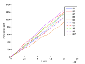
(a) w/0 VLS

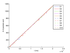
(b) VLS

Figure 3: Improvement of short-term and long-term fairness (10 stations, $W_{j}=1,\forall j$) (Throughout the paper, “S1” means “Station 1”, etc.)

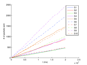
(a) w/o VLS (The vector of $CW_{min}$’s of the 10 stations is (128 64 128 64 42 32 128 64 26 42))

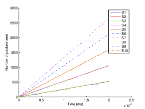
(b) VLS (The vector of weights of the 10 stations is (1 2 1 2 3 4 1 2 5 3))

Figure 4: Weighted Fairness

III-C Solving Unfairness Problems

Besides improving short-term fairness and providing weighted fairness, our algorithm can readily solve many other unfairness problems in wireless networks.

III-C1 Unfairness due to Capture Effect

In a WLAN, different stations may have very different distances from the AP. Also, the channel qualities between stations and the AP may differ greatly even if the distances are similar, for instance because of multipath or obstructions. The above effects result in different signal strengths from different stations as received by the AP. When more than one stations transmit packets to the AP at the same time , so that these transmissions collide, the AP may still be able to capture and correctly decode the packet with the strongest signal, and send back an ACK. This feature is helpful in terms of the aggregate throughput since one packet is received even in the event of a collision, but may exacerbate the unfairness. The weaker stations tend to backoff more with the BEB algorithm, and therefore obtain much less throughput than stronger ones (see Fig. 5(a)).

If our VLS algorithm is enabled, it can overcome the unfairness problem, as well as retaining the throughput benefit provided by capture. Since both strong and weak stations share the same view of the virtual slots, they share the bandwidth in a fair way (see Fig. 5(b)).

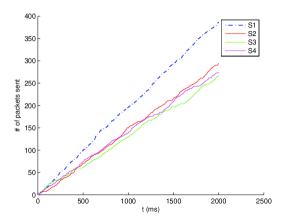
(a) w/o VLS

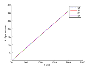
(b) VLS

Figure 5: Overcoming unfairness due to capture effect (S1 is the strong station. When S1’s packets collide with other stations’ packets, S1’s packet is captured)

III-C2 Unfairness due to Channel Errors

In wireless networks, in addition to packet collisions, channel errors are another important cause of packet losses. If a station has a lossy channel to the AP, its packets are dropped with higher probability because of channel errors. Similarly to the capture effect, these losses also result in an asymmetry among different stations, and therefore in unfairness, aggravated by the BEB algorithm. This effect is shown in Fig. 7(a) where only station 1 suffers from a loss probability $p=0.15$ caused by channel errors.

A simple model of a time-varying wireless channel is a Markov chain with two states: “good” and “bad”. For simplicity, we assume that in the “good” state all packets can be received and that in the “bad” state all packets are dropped. Each state has an exponentially-distributed duration before it transits to the other state. Fig. 6 shows the state transition diagram. In the scenario simulated, only station 1 has such a noisy channel, with $\lambda_{g}=20/sec$, $\lambda_{b}=113/sec$ (therefore the average loss probability is $p=0.15$); and other stations have perfect channels ($p=0$). It turns out that our algorithm not only maintains fairness, but also utilize the channel “opportunistically” to get a high throughput: When the weak station wins a contention, but meets the “bad” state, it transmits a packet, without receiving the ACK, and relinquishes the channel immediately. When it wins a contention and meets the “good” state, it can transmit a burst of packets. Since the channel is likely to stay in the “good” state for some time, the station has the opportunity to compensate for its past losses. If at some point the state goes back to “bad”, the station stops immediately and waits for the next opportunity (see Fig. 7(b)). In other words, the weak station transmits more when the channel is good, and less when the channel is bad, thus utilizing the noisy channel more efficiently. As a result, the total throughput in Fig. 7(b) is only slightly less than that in Fig. 7(c), where the channels are perfect for all stations.

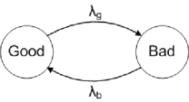
Figure 6: Markov Channel Model

It is evident that if the average duration of the “good” state is too short, the weak station may still receive unfair throughput. We can derive the condition under which fairness is guaranteed (see Section IV). Nevertheless, VLS always improves the fairness.

When the channel of one station is significantly worse than that of the others, providing throughput-fairness to different stations may drag down the total throughput of the network. (This is a tradeoff between fairness and efficiency.) In that case, providing time-fairness would be more suitable. VLS has the flexibility to provide time-fairness, as mentioned in subsection II-D.

In the above, we have assumed that the stations do not know the state of the channel before transmitting. If the channel state information is known in advance, the station can avoid transmitting in the “bad” state. In that case, the throughput performance is further improved.

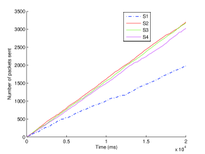
(a) w/o VLS, only S1 suffers a loss rate $p$=0.15 due to channel errors

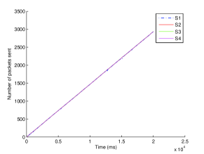
(b) With VLS, $p$=0.15 for S1

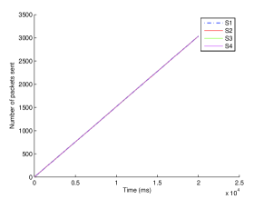
(c) With VLS, $p$=0 for all stations

Figure 7: Overcoming unfairness due to channel errors (Note that in (b) fairness is achieved, also, the throughput is close to (c) w/o channel errors.)

IV Stability of the Credits

In VLS, each active station keeps accumulating and spending credit, where the accumulated credit is proportional to a station’s weight, the number of virtual slots it has observed, and the speed of clock $c$. In this section, we consider whether the credits are stable, that is, whether the credits of some stations keep increasing and go to infinity. If that happens, the bandwidth allocation may not be fair, since the extra credits of some stations are not spent.

First, if there is no limit on the length of transmission at each burst, the credits must be stable, given that each station has non-zero probability of winning the channel. Suppose at each virtual slot, a station $i$ has a probability of $p_{i}$ of winning the channel, then on average, it has accumulated $W_{i}\cdot c/p_{i}<\infty$ units of credit. It then spent all of them. In fact, the probability that the credits reach $G$ (before it is spent) is approximately $(1-p_{i})^{G/(W_{i}\cdot c)}$. Therefore $Pr\{G=\infty\}=0$.

But if there is a pre-defined limit of the burst length $B_{i}$ for station $i$, then instability is possible. In particular, if $B_{i}\leq W_{i}\cdot c/p_{i}$, the credits of station $i$ go to infinity. This can be readily proved by law of large numbers. Also, this inequality tells us how to avoid instability: ensuring

$$B_{i}>W_{i}\cdot c/p_{i},\forall i$$ (1)

For implementation, each station monitors its $p_{i}$ (average over a period of time). If the inequality is violated, it computes a proper value of $c$ and broadcasts it to the network. Then every station uses the new value of $c$. Another simple implementation is to monitor the credits. If the credits of station $i$ keep increasing, it knows a smaller $c$ is needed to stabilize its credit.

The above analysis can be extended to the case of capture effect or channel errors.

1. Capture effect. Capture effect will affect the values of the $p_{i}$’s. The weaker stations have smaller $p_{i}$’s, which, in turn, may entail adjustment of $c$.

2. Channel errors. Here, we define $p_{i}$ as station $i$’s probability of winning the contention AND meet the “good” state of channel $i$, in a given virtual slot. Accordingly, channel errors clearly affect the $p_{i}$’s. The stations with noisy channels have smaller $p_{i}$’s (due to both channel errors and BEB). Also, the time-variation of channel quality imposes another limit on the burst length. Denote the length of the “good” period of channel $i$ as $T_{i}$, which is a random variable. Then the following inequality is required:

   $${\bf E}[min(B_{i},T_{i})]>W_{i}\cdot c/p_{i},\forall i$$ (2)

To analyze the values of $p_{i}$’s, one can adapt Bianchi’s fixed point model [4]. In practice, the stations do not need to compute $p_{i}$’s. They only need to adjust $c$ according to their extra credits.

V VLS in Multiple Collision domain

If a wireless network has multiple collision domains, a station may not be able to hear all the other stations’ transmissions. Therefore, different stations may have different views of the virtual slots, which makes virtual-slot-based scheduling more difficult. (Two stations have the same view of virtual slots only if they can hear the same set of stations.) In IEEE 802.11, this may cause severe unfairness problem (as will be shown later). So, in this case, we devise a variable-length scheduling algorithm based on the realized throughputs, instead of the number of virtual slots. The basic idea is similar to [3][5]. (There, the minimum Contention Windows, $CW_{min}$’s, are dynamically adjusted.)

Say we have a set of $J$ stations, with respective weights $W_{j},j=1,2,\dots,J$. The weights can be pre-determined by optimizing some global objective of the network. For example, they can be the solution of the utility optimization problem [6][10]

$$max \sum_{j}U_{j}(W_{j})$$

$$st \sum_{k\in{\cal C}_{m}}W_{k}\leq 1,\forall{}_{m},m=1,2,\dots,M$$

where $U_{j}$ is the concave “utility function” of station $j$, and each set ${\cal C}_{m}$ is a “clique” (in a clique, only one station can transmit at a time). Note that with the constraints, we have assumed that the contention graph is a “perfect graph” [12] (otherwise, another set of constraints based on “independent set” should be used [12]). We have also omitted some details such as packet collisions. This optimization problem can be solved in a distributed manner, similar to wired network [6]. A “clique” here is analogous to a “link” in wired network, therefore to solve the problem, some communication among stations in the same clique is needed.

In this VLS algorithm, each station $j$ monitors the aggregate throughput of its neighbors ${\cal N}_{j}$ (i.e, $\sum_{k\in{\cal N}_{j}}S_{k}$), as well as its own throughput $S_{j}$. (This can be done in several ways: (a) station $j$ can overhear the packets sent by its neighbors, if possible; (b) otherwise, stations can explicitly exchange information about their throughput with their neighbors periodically.) Then, it adjusts the burst length as follows.

$$b_{j}(t+1)=b_{j}(t)-\alpha(t)b_{j}(t)(\frac{S_{j}}{\sum_{k\in{\cal N}_{j}}S_{k}}-\frac{W_{j}}{\sum_{k\in{\cal N}_{j}}W_{k}})$$

where $b_{j}(t)$ denotes the burst length of station $j$ at time $t$, and $\alpha(t)$ is the step size. Clearly, $b(t)$ converges when the actual ratio of throughputs is equal to the target ratio of weights.

In the following simulation, we compare the throughput allocation with fixed-length scheduling and VLS. In VLS, we use a discrete version of the above algorithm: each node adjusts its transmission length every 4ms, and the throughput $S_{j}$ is an average over the last 40ms.

In the network simulated, stations 1, 2, 3 belong to Collision Domain 1, while stations 3, 4, 5 belong to Collision Domain 2, as shown in Fig. 8(a). Note that station 3 faces contentions from both domains. The destinations of the flows from node 1, 2, 3, 4, 5 are assumed to be node 2, 1, 2, 5, 4, respectively. The data rate is 11Mbps, and the initial transmission length is 1ms for all stations.

Without VLS, station 3’s throughput is very low compared to others (Fig. 8(b)). The reason is that at most of the time, station 3 senses the medium as busy, due to the transmissions in both collision domains. Therefore it does not have much chance to transmit its packets. Then, we use VLS, and require the weights of all stations to be 1/3. As shown in Fig. 8(c), after a short period of time in the beginning (for convergence), the target weights are achieved. On average, station 3’ transmission length is 1.54ms, while others’ are about 0.5ms after convergence.

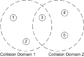
(a) A network with 2 collision domains

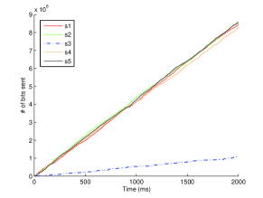
(b) Without VLS

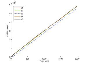
(c) VLS, with equal weights for all stations

Figure 8: VLS in Multiple Collision Domains

VI Conclusions

In this paper, we have proposed a distributed algorithm, VLS, for fair scheduling in 802.11 wireless networks. We have shown that, by varying the transmission lengths of different stations, it is feasible to provide fairness without careful modeling of MAC-layer contention, physical channel variations, and the effect of multiple collision domains. Many existing fairness problems in 802.11 networks are therefore overcome, including short-term unfairness, unfairness introduced by physical channel’s asymmetry, such as capture effect and channel errors. It makes the throughput of each station more smooth, which is appealing to real-time service such as video and voice. It can easily provide weighted fairness for different services. For networks with multiple collision domains, VLS gives a way to avoid the starvation of those stations that are in several collision domains.

Since VLS can avoid excessively long transmissions by tuning the parameter $c$, we should be able to achieve certain objectives on packet delay. However, this problem has not been studied thoroughly in this paper, and is a subject for further study.

Since VLS can be used in 802.11e networks, the advantages of both protocols can be achieved: VLS can provide weighted fairness (a prioritization) in terms of throughput, while 802.11e can provide prioritization in terms of delay, by using different $CW_{min}$’s and IFS’s (Inter-Frame Spaces). Therefore, throughputs and delays can be controlled separately by two protocols, instead of being coupled in a complicated way as in 802.11e [13]. More analytical/experimental study of this issue is interesting for future research.

References

- [1] Information technology- telecommunications and information exchange between systems- local and metropolitan area networks- specific requirements- part 11: Wireless lan medium access control (mac) and physical layer (phy) specifications. ANSI/IEEE Std 802.11, 1999 Edition (R2003), pages i–513, 2003.
- [2] Unapproved draft amendment standard for information technology– telecommunications and information exchange between systems–lan/man specific requirements– part 11 wireless medium access control (mac) and physical layer (phy) specifications: Medium access control (mac) quality of service (qos) enhancements (replaced by approved draft 802.11e/d13.0). IEEE Std P802.11e/D13.0, 2005.
- [3] B. Bensaou, Wang Yu, and Ko Chi Chung. Fair medium access in 802.11 based wireless ad-hoc networks. In Mobile and Ad Hoc Networking and Computing, 2000. MobiHOC. 2000 First Annual Workshop on, pages 99–106, 2000.
- [4] G. Bianchi. Performance analysis of the ieee 802.11 distributed coordination function. Selected Areas in Communications, IEEE Journal on, 18(3):535–547, 2000. 0733-8716.
- [5] Rajarshi Gupta and Jean Walrand. Achieving Fairness in a Distributed Ad-Hoc MAC. ”Advances in Control, Communication Networks, and Transportation Systems,” E.H. Abed (Ed.), Systems and Control: Foundations and Applications Series, Springer-Birkhauser, Boston. July 2005.
- [6] F. Kelly. Charging and rate control for elastic traffic. European Transactions on Telecommunications, 8:33–37, January 1997.
- [7] A. Kochut, A. Vasan, A. U. Shankar, and A. Agrawala. Sniffing out the correct physical layer capture model in 802.11b. In Network Protocols, 2004. ICNP 2004. Proceedings of the 12th IEEE International Conference on, pages 252–261, 2004.
- [8] C. T. Lau and C. Leung. Capture models for mobile packet radio networks. Communications, IEEE Transactions on, 40(5):917–925, 1992. 0090-6778.
- [9] Jiang Li Bin and Liew Soung Chang. Proportional fairness in wireless lans and ad hoc networks. In Wireless Communications and Networking Conference, 2005 IEEE, volume 3, pages 1551–1556 Vol. 3, 2005.
- [10] X. Lin, N.B. Shroff, and R. Srikant. A tutorial on cross-layer optimization in wireless networks. Selected Areas in Communications, IEEE Journal on, 24(8):1452–1463, 2006.
- [11] Liew S.C Qixiang Pang, Leung V.C.M. Improvement of WLAN contention resolution by loss differentiation. IEEE Transactions on Wireless Communications, 5:3605 – 3615, December 2006.
- [12] John Musacchio Rajarshi Gupta and Jean Walrand. Sufficient rate constraints for QoS flows in ad-hoc networks. AD HOC NETWORKS, 5(4):429–443, May 2007.
- [13] J. W. Robinson and T. S. Randhawa. Saturation throughput analysis of ieee 802.11e enhanced distributed coordination function. Selected Areas in Communications, IEEE Journal on, 22(5):917–928, 2004. 0733-8716.
- [14] Choi Sunghyun, J. del Prado, N. Sai Shankar, and S. Mangold. ”IEEE 802.11 e contention-based channel access (EDCF) performance evaluation”. In Communications, 2003. ICC ’03. IEEE International Conference on, volume 2, pages 1151–1156 vol.2, 2003.
- [15] N. Vaidya, A. Dugar, S. Gupta, and P. Bahl. Distributed fair scheduling in a wireless LAN. Mobile Computing, IEEE Transactions on, 4(6):616–629, 2005.