Continuum limits of random matrices
and the Brownian carousel

Abstract

We show that at any location away from the spectral edge, the eigenvalues of the Gaussian unitary ensemble and its general $\beta$ siblings converge to $\operatorname{Sine}_{\beta}$, a translation invariant point process. This process has a geometric description in term of the Brownian carousel, a deterministic function of Brownian motion in the hyperbolic plane.

The Brownian carousel, a description of the a continuum limit of random matrices, provides a convenient way to analyze the limiting point processes. We show that the gap probability of $\operatorname{Sine}_{\beta}$ is continuous in the gap size and $\beta$, and compute its asymptotics for large gaps. Moreover, the stochastic differential equation version of the Brownian carousel exhibits a phase transition at $\beta=2$.

The Brownian carousel and the winding angle $\alpha_{\lambda}$

1 Introduction

The Gaussian orthogonal and unitary ensembles are the most fundamental objects of study in random matrix theory. In the past decades, their eigenvalue distribution has shown to be important in several areas of probability, combinatorics, number theory, operator algebras, even engineering (see Deift (1999) for an overview). For dimension $n$, the ordered eigenvalues $\lambda_{1}\leq\ldots\leq\lambda_{n}\in{\mathbb{R}}$ have joint density

$$\frac{1}{Z_{n,\beta}}\;e^{-\beta\sum_{k=1}^{n}\lambda_{k}^{2}/4}\,\prod_{j<k}|\lambda_{j}-\lambda_{k}|^{\beta},$$ (1)

where $\beta=1,2$ for the Gaussian orthogonal and unitary ensembles, respectively. The above density makes sense for any $\beta\geq 0$, and the point process is often called Coulomb gas in Gaussian potential at inverse temperature $\beta$. The goal of this paper is to study its $n\to\infty$ point process limit away from the spectral edge.

The limit is described via a special case of the hyperbolic carousel. Let

• $b$ be a path in the hyperbolic plane

• $z$ be a point on the boundary of the hyperbolic plane, and

• $f:{\mathbb{R}}_{+}\to{\mathbb{R}}_{+}$ be an integrable function.

To these three objects, the hyperbolic carousel associates a multi-set of points on the real line defined via its counting function $N(\lambda)$ taking values in ${\mathbb{Z}}\cup\{-\infty,\infty\}$. As time increases from $0$ to $\infty$, the boundary point $z$ is rotated about the center $b(t)$ at angular speed $\lambda f(t)$. $N(\lambda)$ is defined as the integer-valued total winding number of the point about the moving center of rotation.

The Brownian carousel is defined as the hyperbolic carousel driven by hyperbolic Brownian motion $b$. See Section 2 for more details.

In order to study the $n\to\infty$ limit of (1) we need to pick the center $\mu_{n}$ of the scaling window for each $n$. Then the scaling factor follows the Wigner semicircle law. Our main theorem gives necessary and sufficient conditions on $\mu_{n}$ to get a bulk-type limit.

Theorem 1.

For $\beta>0$, let $\Lambda_{n}$ denote the point process given by (1), and let $\mu_{n}$ be a sequence so that  $n^{\nicefrac{{1}}{{6}}}(2\sqrt{n}-|\mu_{n}|)\to+\infty$. Then

$$\sqrt{4n-\mu_{n}^{2}}\big{(}\Lambda_{n}-\mu_{n}\big{)}\Rightarrow\operatorname{Sine}_{\beta},$$

where ${\rm Sine}_{\beta}$ is the discrete point process given by the Brownian carousel with parameters $f(t)=(\beta/4)e^{-\beta t/4}$ and arbitrary $z$.

The convergence here is in law with respect to vague topology for the counting measure of the point process. The limit and convergence for the special values $\beta=1,2,4$ under more restrictive scaling conditions has been well-studied, see Mehta (2004) or Forrester (2008). The Brownian carousel description is novel even in these special cases. We note that the ensemble (1) may be generalized by replacing the $\sum_{k}\lambda_{k}^{2}$ in the exponent by a similar sum involving a fixed function $V$ of the eigenvalues. Assuming certain growth conditions on $V$ the corresponding problem in the $\beta=2$ case can be treated using orthogonal polynomials and Riemann-Hilbert methods, see e.g. Deift (1999), Deift et al. (1999).

Together with the following theorem, Theorem 1 gives a complete characterization of the possible limiting processes for the ensembles (1).

Theorem 2 (Ramírez, Rider, and Virág (2007)).

For $\beta>0$, let $\Lambda_{n}$ denote the point process given by (1), and let $\mu_{n}$ be a sequence so that $n^{\nicefrac{{1}}{{6}}}(2\sqrt{n}-\mu_{n})\to a\in{\mathbb{R}}$. Then

$$n^{\nicefrac{{1}}{{6}}}(\Lambda_{n}-\mu_{n})\Rightarrow\operatorname{Airy}_{\beta}+\,a$$

Here $\operatorname{Airy}_{\beta}$ is defined as $-1$ times the point process of eigenvalues of the stochastic Airy operator, see Ramírez, Rider, and Virág (2007)  for more details. A straightforward diagonalization argument gives the following corollary, which is proved in Section 3.

Corollary 3.

As $a\to\infty$ we have $2\sqrt{a}(\operatorname{Airy}_{\beta}+a)\Rightarrow\operatorname{Sine}_{\beta}$.

The proof of Theorem 1 is based on the tridiagonal matrix models introduced by Trotter (1984) and Dumitriu and Edelman (2002). Sutton (2005) and Edelman and Sutton (2007) present heuristics that the operators given by the tridiagonal matrices have a limit whose eigenvalues give the Sine and Airy processes. Theorem 2 shows that this is indeed the case at the spectral edge. The bulk case, however, is fundamentally different: there seems to be no natural limiting operator with the spectrum given by the Sine point process. Rather than taking a limit of the operator itself, we consider limits of discrete variants of the phase functions in the Sturm-Liouville theory. This connection is explored further in Section 5.3, where we describe how the Sine point process appears as a universal limit for a large class of one-dimensional Schrödinger operators.

The eigenvalue equation of a real tridiagonal matrix gives a three-term linear recursion for the eigenvectors. This becomes a two-term recursion for the ratios of consecutive entries, which then evolves by linear fractional transformations fixing the real line. So in our case, the evolution operators perform a time-inhomogeneous random process in $\operatorname{PSL}(2,{\mathbb{R}})$, the group of orientation-preserving isometries of the hyperbolic plane. To get the Brownian carousel, we regularize this evolution and take limits. An important tool is Proposition 23 (based on the results of Stroock and Varadhan (1979)), which yields stochastic differential equation limits of Markov processes with heavy local oscillations.

The Brownian carousel description gives a simple way to analyze the limiting point process. The hyperbolic angle of the rotating boundary point as measured from $b(t)$ follows the stochastic sine equation, a coupled one-parameter family of stochastic differential equations

$$d\alpha_{\lambda}=\lambda f\,dt+\operatorname{Re}((e^{-i\alpha_{\lambda}}-1)dZ),\qquad\alpha_{\lambda}(0)=0,$$ (2)

driven by a two-dimensional standard Brownian motion. For a single $\lambda$, this reduces to the one-dimensional stochastic differential equation

$$d\alpha_{\lambda}=\lambda f\,dt+2\sin(\alpha_{\lambda}/2)dW,\qquad\alpha_{\lambda}(0)=0,$$ (3)

which converges as $t\to\infty$ to an integer multiple $\alpha_{\lambda}(\infty)$ of $2\pi$. A direct consequence of the definition of $\operatorname{Sine}_{\beta}$ is the following.

Proposition 4.

The number of points $N(\lambda)$ of the point process $\operatorname{Sine}_{\beta}$ in $[0,\lambda]$ has the same distribution as $\alpha_{\lambda}(\infty)/(2\pi)$.

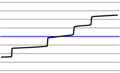
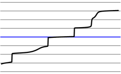
MM MM

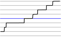
Figure 1: The $\beta=1$ stochastic sine equation as a function of $\lambda$ at three times

Convergence to the solution of the coupled SDEs is the result formally announced in the lecture by Virág (2006). In independent work, Killip and Stoiciu (2006) present a related but different description of the limit processes in the setting of circular ensembles (see, e.g. Forrester (2008), Chapter 2 for discussion of these models and Killip (2007) for further related results).

Proposition 4 allows us to analyze the point process $\operatorname{Sine}_{\beta}$, for example to determine the asymptotics of large gap probabilities. This has been predicted by Dyson (1962) and proved for the cases $\beta=2$ by Widom (1996) and for $\beta=1,4$ by Jimbo et al. (1980); there, more refined asymptotics are presented; see also Deift et al. (1997).

Theorem 5.

For $k\geq 0$ fixed and $\lambda\to\infty$, we have

$$\mbox{\rm P}(\mbox{\# of points in }[0,\lambda]\leq k)=\exp\big{(}-\lambda^{2}(\beta/64+o(1))\big{)}.$$

This is shown in Section 2.3 for the case of a more general parameter $f$. Several similar asymptotic identities can be computed this way, and continuity properties can be studied. For the $\operatorname{Sine}_{\beta}$ processes we have

Proposition 6.

The probability distribution of $N(\lambda)$ is a continuous function of $\lambda$ and $\beta$.

In contrast, the stochastic sine equation exhibits a phase transition at $\beta=2$.

Theorem 7.

For any $\lambda>0$ we have a.s.

$$\mbox{for all }t\mbox{ large enough }\alpha_{\lambda}(t)\geq\alpha_{\lambda}(\infty)$$ (4)

if and only if $\beta\leq 2$. In particular, the probability of the event (4) is not analytic at $\beta=2$ as a function of $\beta$.

Deift (personal communication, 2007) asked whether this phase transition also appears on the level of gap probabilities. This question remains open.

2 The Brownian carousel and the stochastic sine equation

2.1 Definitions

In the Poincaré disk model of the hyperbolic plane a boundary point can be described by an angle. The Brownian carousel ODE with parameters $f(t)$ and $z_{0}$ describes the evolution of the lifted angle $\gamma_{\lambda}(t)$ with $e^{i\gamma_{\lambda}(0)}=z_{0}$ as it is rotated about the center $B(t)$ at angular speed $\lambda f(t)$. Here $B(t)$ is hyperbolic Brownian motion, that is the strong solution of the SDE

$$\qquad dB=\frac{(1-|B|^{2})}{2}\,d\tilde{Z}$$

driven by complex Brownian motion $\tilde{Z}$ with standard real and imaginary parts. The speed of $\gamma_{\lambda}$, as measured in units of boundary harmonic measure from $B$, is $\lambda f/(2\pi)$. To change to an angle measured from $0$, we need to divide by the Poisson kernel

$$\mbox{\rm Poi}(e^{i\gamma_{\lambda}},w)=\frac{1}{2\pi}\operatorname{Re}\,\frac{e^{i\gamma_{\lambda}}+w}{e^{i\gamma}-w}=\frac{1}{2\pi}\frac{1-|w|^{2}}{|e^{i\gamma_{\lambda}}-w|^{2}},$$

which yields the ODE

$$\partial_{t}\gamma_{\lambda}=\frac{\lambda f}{2\pi\,\mbox{\rm Poi}(e^{i\gamma_{\lambda}},B)}=\lambda f\frac{|e^{i\gamma_{\lambda}}-B|^{2}}{1-|B|^{2}}.$$ (5)

The most convenient way to define the winding number $N(\lambda)$ of $e^{i\gamma_{\lambda}}$ about the moving center of rotation $B(t)$ is to follow the corresponding angle. Let $\alpha_{\lambda}(t)$ denote the hyperbolic angle determined by the points $z_{0},B(t)$ and $e^{i\gamma_{\lambda}(t)}$. As we will check at the end of this section, Itô’s formula shows that $\alpha$ satisfies the stochastic sine equation (2), i.e.

$$d\alpha_{\lambda}=\lambda f\,dt+\operatorname{Re}((e^{-i\alpha_{\lambda}}-1)dZ),\qquad\alpha_{\lambda}(0)=0,$$ (6)

where $dZ$ is simply complex white noise with standard real and imaginary parts. The name of the SDE comes from the fact that the last term equals $2\sin(\alpha_{\lambda}/2)\operatorname{Im}(e^{-i\alpha_{\lambda}/2}dZ)$. Since $dW=\operatorname{Im}(e^{-i\alpha_{\lambda}/2}dZ)$ is 1-dimensional white noise, we get the SDE (3) for the single $\lambda$ marginals.

Propostion 9 of the next section shows that

$$\frac{1}{2\pi}\lim_{t\to\infty}\alpha_{\lambda}(t)$$ (7)

exists for every $\lambda$ a.s. and for every $\lambda_{1}<\lambda_{2}$ a.s. $N({\lambda_{1}})\leq N({\lambda_{2}})$. Thus $N(\lambda)$ can be defined as the unique random right-continuous function which agrees with (7) for every $\lambda$ a.s.

To deduce (6), let ${\mathcal{T}}(w,z)$ denote the Möbius automorphism of the unit disk taking $z_{0}$ to $1$ and taking $w$ to $0$. It is given by the formula

$${\mathcal{T}}(w,z)=\frac{S(w,z)}{S(w,z_{0})},\qquad S(w,z)=\frac{z-w}{1-\overline{w}z}.$$ (8)

Then $\alpha$ is defined as the continuous solution of

$$\alpha(0)=0,\qquad e^{i\alpha(t)}={\mathcal{T}}(B_{t},e^{i\gamma(t)}).$$ (9)

The stochastic sine equation (6) follows from taking logarithms and applying Itô’s formula. For the driving Brownian motion we get the explicit expression

$$dZ={2\partial_{2}{\mathcal{T}}(B,B)}dB=\frac{2}{1-|B|^{2}}\;\frac{1-\overline{B}}{1-B}\ dB.$$

Remark 8.

By Itô’s formula applied to the logarithm of (9), the noise term in (6) can be interpreted as the infinitesimal movement of the angle $\alpha$ under the difference of transformations $d{\mathcal{T}}={\mathcal{T}}(B+dB,\gamma){\mathcal{T}}(B,\gamma)^{-1}$. This infinitesimal Möbius transformation $d{\mathcal{T}}$ moves 0 to ${\mathcal{T}}(B,B+dB)=\partial_{2}{\mathcal{T}}(B,B)dB$, a standard complex Brownian motion increment. Such a transformation $d{\mathcal{T}}$ changes the angle of any two points on the boundary by a Brownian increment with standard deviation proportional to their distance. This gives a more conceptual explanation of the noise term in (6).

2.2 Properties of the Brownian carousel

Let $L^{1}_{*}$ denote the set of absolutely integrable functions of ${\mathbb{R}}^{+}$ which tend to $0$ at $+\infty$. Given a hyperbolic Brownian motion and a boundary point $z_{0}$, the Brownian carousel associates a random counting function $N(\lambda)$ to each $f\in L^{1}_{*}$. More generally, it is fruitful to study how $N(\lambda)$ changes when the parameter $f$ varies but the Brownian path remains fixed. In this case $\lambda$ can be absorbed in the parameter $f$ so we will use the notation $N_{f}=N_{f}(1)$, and $\alpha_{f}$ for the case $\lambda=1$.

Proposition 9 (Properties of the Brownian carousel).

We have

1. $\alpha_{f}-\alpha_{g}$ has the same distribution as $\alpha_{f-g}$,

2. $\alpha_{f}(t)$ is increasing in $f$,

3. $\left\lfloor\alpha_{f}(t)\right\rfloor_{2\pi}$ is nondecreasing in $t$ when $f\geq 0$. Here $\left\lfloor x\right\rfloor_{2\pi}=\max\left(2\pi{\mathbb{Z}}\cap(-\infty,x]\right)$.

4. $N_{f}=\frac{1}{2\pi}\lim_{t\to\infty}\alpha_{f}(t)$ exists and is an integer a.s.,

5. $N_{0}=0$ and $N_{f}$ is increasing in $f$,

6. ${\rm E}|N_{f}|\leq\frac{1}{2\pi}\|f\|_{1},$

7. ${\rm E}N_{f}=\frac{1}{2\pi}\int_{0}^{\infty}f(x)\,dx$, and

8. $N_{f}$ has exponential tails. For integers $a,k>0$ we have

   $$\mbox{\rm P}(|N_{f}|\geq ak)\leq 2\left[\frac{\|f\|_{1}}{2\pi a}\right]^{k}.$$

Proof.

Claim (i) holds because $\alpha_{f}-\alpha_{g}$ solves

$$d\alpha_{\lambda}=\lambda(f-g)\,dt+\operatorname{Re}((e^{-i\alpha_{\lambda}}-1)dZ^{*}),\qquad\alpha_{\lambda}(0)=0,$$

with $dZ^{*}=e^{-i\alpha_{g}}dZ$. The standard coupling argument shows that the solution of the stochastic sine equation is monotone in the drift term, so we get (ii).

Now assume that $f\geq g\equiv 0$. Then by the above $\alpha_{f}(t)\geq\alpha_{g}(t)=0$. Claim (iii) follows by repeating this argument for the process after the hitting time of $2k\pi$.

Assume $f\geq 0$, and let $F(t)=\int_{0}^{t}f(s)\,ds$. Then $\alpha_{f}-F$ is a continuous local martingale which is uniformly bounded below by $-\|f\|_{1}$. Thus it a.s. converges to a random limit. So $\alpha$ also converges, but it can only converge to a location where the noise term vanishes; we get (iv), and (v) also follows from (ii). Now (vi) follows from

$$2\pi{\rm E}N_{f}-\|f\|_{1}={\rm E}\alpha_{f}(\infty)-F(\infty) \leq \lim_{t\to\infty}({\rm E}\alpha_{f}(t)-F(t))$$

$$= \alpha_{f}(0)-F(0)=0,$$

where the inequality is by Fatou’s Lemma. By (iii) the function $t\mapsto\left\lfloor\alpha_{f}(t)\right\rfloor_{2\pi}$ is nondecreasing, hence the above inequality implies that $\left\lfloor\alpha_{f}(t)\right\rfloor_{2\pi}$ is uniformly integrable, and so is $\alpha_{f}(t)$. Thus $\alpha_{f}-F$ is a uniformly integrable martingale and so ${\rm E}\alpha_{f}(\infty)=F(\infty)$, as required for (vii).

For general $f\in L^{1}_{*}$, monotonicity (ii) gives

$$\alpha_{-f^{-}}\leq\alpha_{f}\leq\alpha_{f^{+}},$$ (10)

where $x^{+}=\max(x,0)$ and $x^{-}=(-x)^{+}$. Now $\alpha_{-f^{-}}$ has the same distribution as $-\alpha_{f^{-}}$. By the previous argument $\alpha_{f^{+}}$ and $\alpha_{f^{-}}$ are uniformly integrable. Hence $\alpha_{f}-F$ is a uniformly integrable martingale, and (iv), (vii) follow. Claim (v) also follows via (ii). We take positive and negative part of (10) to get $\alpha_{f}^{+}\leq\alpha_{f^{+}}$, and $\alpha_{f}^{-}\leq-\alpha_{-f^{-}}$, where the latter has the same distribution as $\alpha_{f^{-}}$. Taking limits and expectations gives

$${\rm E}|\alpha_{f}(\infty)|={\rm E}\alpha_{f}(\infty)^{+}+{\rm E}\alpha_{f}(\infty)^{-}\leq{\rm E}\alpha_{f^{+}}(\infty)+{\rm E}\alpha_{f^{-}}(\infty)=\|f\|_{1}$$

which gives (vi).

Returning to $f\geq 0$, Markov’s inequality implies that $\mbox{\rm P}(N_{f}\geq a)\leq\frac{1}{2\pi}\|f\|_{1}/a$. Stopping the process at time $\tau$ when and if $\alpha$ hits $2\pi ka$ we note that

$$\mbox{\rm P}\left(N_{f}\geq(k+1)a\,\big{|}\,N_{f}\geq ka,\mathcal{F}_{\tau}\right)\leq\frac{1}{2\pi}\|f_{\tau}\|_{1}/a\leq\frac{1}{2\pi}\|f\|_{1}/a,$$

where $f_{\tau}$ is $f$ shifted to the left by $\tau$. It follows that for integer $k$ we have

$$\mbox{\rm P}(N_{f}\geq ka)\leq\big{[}\frac{1}{2\pi}\|f\|_{1}/a\big{]}^{k}$$

For general $f\in L^{1}_{*}$, we consider the positive and negative parts separately and use monotonicity (v) to get (viii). ∎

Remark 10.

The previous lemma shows that for a fixed $f\in L^{1}_{*}$ the random function $N(\lambda)$ is a.s. finite, integer valued, monotone increasing with stationary increments. Thus $N(\lambda)$ is the counting function of a translation invariant point process. Since $f\mapsto\alpha_{f}$ and $f\mapsto-\alpha_{-f}$ have the same distribution, the distribution of the point process is symmetric with respect to reflections.

Corollary 11.

For any $f\in L^{1}_{*}$ the point process defined by $N(\lambda)$ is a.s. simple.

Proof.

The tail estimate of the lemma implies that the probability that there are two points or more in a fixed interval of length $\varepsilon$ is at most $c\varepsilon^{2}$. Breaking the interval $[0,1]$ into pieces of length $\varepsilon$, and using translation invariance, we see that the chance that there is a double point in $[0,1]$ is at most $2c\varepsilon$. Letting $\varepsilon\to 0$ shows that a.s. there are no double points in $[0,1]$. The claim now follows from translation invariance. ∎

Let $\mathcal{M}$ denote the space of probability distributions on ${\mathbb{Z}}$ with expectation. For $\mu_{1},\mu_{2}\in\mathcal{M}$ let $d(\mu_{1},\mu_{2})$ be the first Wasserstein distance, i.e. the infimum of ${\rm E}|X_{1}-X_{2}|$ over all realizations where the joint distribution of $(X_{1},X_{2})$ has marginals $\mu_{1}$ and $\mu_{2}$. The topology induced by $d$ is stronger than weak convergence of probability measures. Let $\mathcal{L}(N_{f})$ denote the distribution of $N_{f}$. The following proposition is a stronger version of Proposition 6 in the introduction.

Proposition 12.

The map $f\mapsto\mathcal{L}(N_{f})$ is Lipschitz-1 continuous in $f$: for $f,g\in L^{1}_{*}$ we have $d(\mathcal{L}(N_{f}),\mathcal{L}(N_{g}))\leq\|f-g\|_{1}$.

Proof.

Proposition 9 gives that $N_{g}-N_{f}$ has the same distribution as $N_{g-f}$ which implies

$$d(\mathcal{L}(N_{f}),\mathcal{L}(N_{g}))\leq{\rm E}|N_{g}-N_{f}|={\rm E}|N_{g-f}|\leq\|g-f\|_{1}.\qed$$

2.3 Large gap probabilities

Theorem 13.

Let $f:{\mathbb{R}}^{+}\to{\mathbb{R}}^{+}$ satisfy $f(t)\leq c/(1+t^{2})$ for all $t$ and $\int_{0}^{\infty}|df|<\infty$. Let $k\geq 0$. As $\lambda\to\infty$, for the point process given by the Brownian carousel with parameter $f$ we have

$$\mbox{\rm P}(\mbox{\# of points in }[0,\lambda]\leq k)=\exp\big{(}-\lambda^{2}(\|f\|_{2}^{2}/8+o(1))\big{)}.$$ (11)

Lemma 14.

Let $Y$ be an adapted stochastic process with $|Y_{t}|<m$, and let $X$ satisfy the SDE $dX=YdB$ where $B_{t}$ is a Brownian motion. Then for each $a,t>0$ we have

$$\mbox{\rm P}(X(t)-X(0)\geq a)\leq\exp\left(-a^{2}/(2tm^{2})\right).$$

Proof.

We may assume $X(0)=0$. Then $X_{t}=B_{\tau}$ where $\tau$ is the random time change $\tau=\int_{0}^{t}Y^{2}(s)ds$. Since $\tau<m^{2}t$ the inequality now follows from

$$\mbox{\rm P}(B_{r}>a)\leq\exp\left(-a^{2}/(2r)\right).\qed$$

Proof of Theorem 13.

The event in (11) is given in terms of the stochastic sine equation as $\lim_{t\to\infty}\alpha_{\lambda}(t)\leq 2k\pi$. We will give upper and lower bounds on its probability.

Upper bound. By Proposition 9 (iii) it is enough to give an upper bound on the probability that $\alpha$ stays less than $x=2(k+1)\pi$. For $0<s<t$ we have

$$\mbox{\rm P}(\alpha(t)<x\,|\,\mathcal{F}_{s}) = \mbox{\rm P}\left(-\int_{s}^{t}2\sin(\alpha/2)dB\,>\,\lambda\int_{s}^{t}fdt-x+\alpha(s)\,\Big{|}\,\mathcal{F}_{s}\right).$$

We may drop the $\alpha(s)$ from the right hand side and use Lemma 14 with $Y=-2\sin(\alpha/2)$, $m=2$, $a=\lambda(\int_{s}^{t}fdt-x/\lambda)$ to get the upper bound

$$\mbox{\rm P}(\alpha(t)<x\,|\,\mathcal{F}_{s})\leq\exp(-\lambda^{2}r(s,t)),\qquad r(s,t)=\frac{(\int_{s}^{t}fdt-x/\lambda)^{2}}{8(t-s)}.$$

Then, by just requiring $\alpha(t)<x$ for times $\varepsilon,2\varepsilon,\ldots\in[0,K]$ the probability that $\alpha$ stays less than $x=2(k+1)\pi$ is bounded above by

$${\rm E}\prod_{k=0}^{K/\varepsilon}\mbox{\rm P}(\alpha((k+1)\varepsilon)<x\,\big{|}\,\mathcal{F}_{k\varepsilon})\leq\exp\Big{\{}-\lambda^{2}\sum_{k=0}^{K/\varepsilon}r(\varepsilon k,\varepsilon k+\varepsilon)\Big{\}}.$$

A choice of $\varepsilon$ so that $x/\lambda=o(\varepsilon)$ as $\lambda\to\infty$ yields the asymptotic Riemann sum

$$\sum_{k=0}^{K/\varepsilon}r(\varepsilon k,\varepsilon k+\varepsilon)=\frac{1}{8}\int_{0}^{K}f^{2}(t)dt+o(1).$$

Letting $K\to\infty$ provides the desired upper bound.

Lower bound. Consider the solution $\tilde{\alpha}(t)$ of (3) with the same driving Brownian motion, but with initial condition $\tilde{\alpha}(0)=\pi$. Then $\tilde{\alpha}\geq\alpha$. For $\varepsilon<\pi/4$, let $A_{s}$ be the event that $\tilde{\alpha}(t)\in(0,\pi+\varepsilon]$ for $t\in[0,s]$. Then

$$\mbox{\rm P}(\alpha(\infty)<2\pi)\geq\mbox{\rm P}(A_{s})\sup_{y\in(0,\pi+\varepsilon)}\mbox{\rm P}(\tilde{\alpha}(\infty)<2\pi\,|\,\tilde{\alpha}(s)=y).$$

The sup is bounded below via Markov’s inequality by

$$1-\frac{\pi+\varepsilon+\lambda\int_{s}^{\infty}f(t)dt}{2\pi}\geq 1/4,$$

where the last inequality holds if $s$ is set to be a large constant multiple of $\lambda$. The event $A_{s}$ is equivalent to $R=\log\tan(\tilde{\alpha}/4)$ staying in the interval $I=(-\infty,\log\tan((\pi+\varepsilon)/4)]$ where the evolution of $R$ is given by Itô’s formula as

$$dR=\frac{\lambda}{2}\,f\cosh R\,dt+\frac{1}{2}\tanh R\,dt+dB,\quad R(0)=0.$$

Let $I^{*}=[-\varepsilon,\log\tan((\pi+\varepsilon)/4)]$, and consider a process $R^{*}$ so that (i) the noise terms of $R$ and $R^{*}$ are the same and (ii) the drift term of $R^{*}$ at every time is greater than the spatial maximum over $I^{*}$ of the drift term of $R$. Let $A^{*}_{s}$ denote the event that for $t\in[0,s]$ we have $R^{*}_{t}\in I^{*}$. On this event $R^{*}\geq R$, and therefore $A_{s}$ also holds. With an appropriate choice of $c$ we may set

$$q(t)=(1/2+c\varepsilon)\lambda f(t)+c\varepsilon,\qquad\qquad dR^{*}=q(t)dt+dB.$$

Let $A^{*}_{s}$ also denote the corresponding set of paths. Girsanov’s theorem gives

$$\mbox{\rm P}(R^{*}\in A^{*}_{s})={\rm E}\left[{\mathbf{1}}(B\in A^{*}_{s})\exp\left(-\frac{1}{2}\int_{0}^{s}q(t)^{2}dt+\int_{0}^{s}q(t)dB(t)\right)\right].$$ (12)

Integration by parts transforms the second integral:

$$q(s)B(s)-\int_{0}^{s}B(t)dq(t)\geq-c\varepsilon\lambda\big{(}f(s)+\int_{0}^{\infty}|df|\big{)}-c\varepsilon\geq-c^{\prime}\varepsilon(1+\lambda)$$

on the event $B\in A^{*}_{s}$. Here we also used that $f$ is bounded. The probability of this event, i.e. that Brownian motion stays in an interval of width $c\varepsilon$, is at least $\exp(-c^{\prime}s/\varepsilon^{2})$. In summary, (12) is bounded below by

$$\exp\left(-c\varepsilon(1+\lambda)-c\,s/\varepsilon^{2}-(1/8+c\varepsilon)\lambda^{2}\|f\|_{2}^{2}\right).$$

The choice $s=c\lambda$, $\varepsilon=\lambda^{-\nicefrac{{1}}{{3}}}$ gives the desired lower bound. ∎

2.4 A phase transition at $\beta=2$

The goal of this section is to prove Theorem 7 that at $\beta=2$ there is a phase transition in the behavior of the stochastic sine equation.

As $\alpha$ converges to an integer multiple of $2\pi$ and it can never go below an integer multiple of $2\pi$ that it has passed (Proposition 9 (iii)), eventually it must converge either from above or from below. Theorem 7 says that $\alpha$ converges from above with probability $1$ if and only if $\beta\leq 2$. Otherwise, it converges from below with positive probability.

Proof.

Case $\beta\leq 2$. It suffices to prove that if $\alpha_{\lambda}(t_{0})\in(2\pi k-y,2\pi k)$ with $0<y<\pi$ then $\alpha_{\lambda}(t)$ leaves this interval a.s. in finite time. As $\alpha_{\lambda}(t+t_{0})$ also evolves according to the stochastic sine equation with $\lambda^{\prime}=\lambda e^{-\beta t_{0}/4}$, we may set $t_{0}=0$ and we are also free to set $k=1$. Let $\mathcal{B}$ denote the event that the process $\alpha_{\lambda}$ started at $\alpha_{\lambda}(0)=x$ in $(2\pi-y,2\pi)$ will stay in this interval forever. It suffices to show that $\mathcal{B}$ has zero probability.

Consider $R=\log\tan(\alpha_{\lambda}/4)$ and set $y$ so that $\log\tan((2\pi-y)/4)=1$. While $\alpha_{\lambda}\in(0,2\pi)$, Itô’s formula gives the evolution of the process $R$:

$$R(0)=r_{0}>1,\qquad dR=q(R,t)dt+dB,\qquad q(r,t)=\frac{\lambda}{2}\,\cosh r\,e^{-\beta t/4}+\frac{1}{2}\tanh r$$ (13)

Then $\mathcal{B}$ is the event that $R(t)\in(1,\infty)$ for all $t$. On $\mathcal{B}$ we have

$$q(R,t)>\frac{1}{2}\tanh R\geq\frac{1}{2}-e^{-2R}\geq 1/4.$$

which gives $R(t)\geq t/4-B(t)+r_{0}$ from (13). Set

$$Q(t)=\int_{0}^{t}\frac{\tanh(R)-1}{2}ds,$$ (14)

by the previous inequality, on the event $\mathcal{B}$ we have

$$Q(t)\geq-\int_{0}^{t}e^{-t/2+2B(s)-2r_{0}}ds>-\int_{0}^{\infty}e^{-t/2+2B(s)-2r_{0}}ds=-M.$$

where the integral $M$ is a.s. finite. Let

$$L(t)=R(t)-t/2-B(t)-Q(t).$$ (15)

Then on $\mathcal{B}$ we have

$$L^{\prime}(t) = \frac{\lambda}{2}\cosh(L(t)+t/2+B(t)+Q(t))e^{-\beta t/4}$$ (16)

$$\geq \frac{\lambda}{4}\exp\left[L(t)+B(t)+t(1/2-\beta/4)-M\right].$$ (17)

The equation follows from Itô’s formula and the inequality uses $\cosh r\geq e^{r}/2$. Multiplying (17) by $e^{-L}$ and integrating we get that on the event $\mathcal{B}$

$$e^{-L(0)}-e^{-L(t)}\geq C\int_{0}^{t}\exp\left[B(s)+s(1/2-\beta/4)\right]ds.$$

with a random $0<C<\infty$. As the exponent is a Brownian motion with nonnegative drift, the limit of the integral on the right is a.s. infinite, thus the probability of $\mathcal{B}$ is 0.

Case $\beta<2$. It suffices to prove that for a large $t_{0}$ if $\alpha_{\lambda}(t_{0})\in(2\pi-\varepsilon,2\pi)$ then $\alpha_{\lambda}(t)$ stays in the slightly larger interval $(2\pi-\delta,2\pi)$ with positive probability. Choosing the values of $\varepsilon$ and $\delta$ appropriately it suffices to show that if $R(0)>2$ and $\lambda$ is small enough then the event $\mathcal{B}$ that $R\in(1,\infty)$ for $t\geq 1$ has positive probability.

Recall the definition of $Q$ and $L$ from (14) and (15). On the event $\mathcal{B}$ we have

$$1/4\leq\tanh(R)\leq 1/2,\quad\textup{and}\quad-t/4\leq Q(t)\leq 0.$$

Using this with (16) and the fact that for $r$ nonnegative $\cosh r\leq e^{r}$ we get

$$L^{\prime}(t) \leq \frac{\lambda}{2}\exp\left[L(t)+B(t)+t(1/2-\beta/4)\right].$$ (18)

From (18) we get

$$e^{-L(0)}-e^{-L(t)}\leq\frac{\lambda}{2}\int_{0}^{t}\exp\left[B(s)+s(1/2-\beta/4)\right]ds.$$

Let $M^{*}$ denote the above integral for $t=\infty$. Then $M^{*}$ is almost surely finite. Moreover, $L(t)$ and thus $R(t)$ remain finite if

$$M^{*}<2e^{-L(0)}/\lambda.$$ (19)

From (16) we get $L^{\prime}(t)>0$ and $L(t)>L(0)=2$ which gives

$$R(t)>2+B(t)+t/2+Q(t)\geq 2+B(t)+t/4.$$

So $R(t)$ stays above 1 if

$$B(t)\geq-t/4-1\qquad\mbox{ for all }t.$$ (20)

This has positive probability, so the conditional distribution of and $M^{*}$ given (20) is supported on finite numbers. This means that the intersection of the events (20) and (19) holds with positive probability for a sufficiently small choice of $\lambda$, and it implies $\mathcal{B}$. ∎

3 Breakdown of the proof of Theorem 1

The goal of this section is to divide the proof of the main theorem into independent pieces, which in turn will be proved in the later sections. The proof presented here also serves as an outline of the later sections.

Proof of Theorem 1.

Fix $\beta>0$, and consider the $n\times n$ random tridiagonal matrix

$$M(n)=\frac{1}{\sqrt{\beta}}\left(\begin{array}[]{cccc}\mathcal{N}_{0}&\chi_{(n-1)\beta}&&\\ \chi_{(n-1)\beta}&\mathcal{N}_{1}&\chi_{(n-2)\beta}&\\ &\chi_{(n-2)\beta}&\mathcal{N}_{2}&\ddots\\ &&\ddots&\ddots\end{array}\right).$$ (21)

where the $\chi_{j\,\beta}$ and $\mathcal{N}_{j}$ entries are independent, $\mathcal{N}_{j}$ has normal distribution with mean 0 and variance 2, and $\chi_{j\beta}$ has chi distribution with $j\beta$ degrees of freedom. (For integer values of its parameter, $\chi_{d}$ is the length of a $d$-dimensional vector with independent standard normal entries.) We let $\Lambda_{n}$ be the multi-set of eigenvalues of this matrix, which by Dumitriu and Edelman (2002) has the desired distribution (1).

First, we may assume that $\mu_{n}\geq 0$; indeed, for a tridiagonal matrix, changing the sign of all diagonal elements changes the spectrum to its negative. In our case the diagonal elements have symmetric distributions, and by Remark 10 the limiting $\operatorname{Sine}_{\beta}$ process is also symmetric.

We set

$$n_{0}=n_{0}(n)=n-\mu_{n}^{2}/4-\frac{1}{2}.$$

The assumption $n^{\nicefrac{{1}}{{6}}}(2\sqrt{n}-|\mu_{n}|)\to\infty$ implies

$$n_{0}^{-1}\mu_{n}^{\nicefrac{{2}}{{3}}}\to 0,\qquad\frac{4n-\mu_{n}^{2}}{4n_{0}}\to 1.$$

So it suffices to show that

$$\textup{if $n_{0}^{-1}\mu_{n}^{\nicefrac{{2}}{{3}}}\to 0$ as $n\to\infty,$\quad then\quad}2n_{0}^{\nicefrac{{1}}{{2}}}(\Lambda_{n}-\mu_{n})\Rightarrow\operatorname{Sine}_{\beta},$$ (22)

an equivalent version of the claim which makes computations nicer. Recall that the counting function $N(\lambda)$ of a set of points in ${\mathbb{R}}$ is the number of points in $(0,\lambda]$ for $\lambda\geq 0$ or negative the number of points in $(\lambda,0]$ for $\lambda<0$.

Denote the counting function of the random multiset $2n_{0}^{\nicefrac{{1}}{{2}}}(\Lambda_{n}-\mu_{n})$ by $N_{n}(\lambda)$, and that of $\operatorname{Sine}_{\beta}$ by $N(\lambda)$. Claim (22) follows if for every $d\geq 1$ and $(\lambda_{1},\lambda_{2},\ldots,\lambda_{d})\in{\mathbb{R}}^{d}$ we have

$$\big{(}N_{n}(\lambda_{1}),N_{n}(\lambda_{2}),\ldots,N_{n}(\lambda_{d})\big{)}\stackrel{{\scriptstyle d}}{{\Longrightarrow}}\big{(}N(\lambda_{1}),N(\lambda_{2}),\ldots,N(\lambda_{d})\big{)}.$$

The proof of this consists of several steps, these are verified in detail in the subsequent sections with the help of the Appendix.

Consider the one-parameter family of SDEs defining the $\operatorname{Sine}_{\beta}$ process:

$$d\tilde{\alpha}_{\lambda}=\lambda\frac{\beta}{4}e^{-\beta t/4}dt+\operatorname{Re}((e^{-i\tilde{\alpha}_{\lambda}}-1)dZ),$$ (23)

where $Z$ is complex Brownian motion on $[0,\infty)$ with standard real and imaginary parts. The time-change $t\to-\frac{2}{\beta}\log(1-t)$ transforms (23) to

$$2\sqrt{\beta(1-t)}\,d\alpha_{\lambda}=\lambda\beta^{\nicefrac{{1}}{{2}}}dt+2\sqrt{2}\operatorname{Re}((e^{-i\alpha_{\lambda}}-1)dW),$$ (24)

where $W_{t}$ is complex Brownian motion for $t\in[0,1)$ with standard real and imaginary parts. Proposition 9 of Section 2 shows that the counting function $N(\lambda)$ of the process $\operatorname{Sine}_{\beta}$ can be represented as the right-continuous version of $(2\pi)^{-1}\lim_{t\to\infty}\tilde{\alpha}_{\lambda}(t)$, a limit which exists for every $\lambda\in{\mathbb{R}}$ a.s. This gives

Step 1.

For every $\lambda\in{\mathbb{R}}$, a.s. we have $2\pi N(\lambda)=\lim_{\varepsilon\to 0^{+}}\alpha_{\lambda}(1-\varepsilon)$.

The eigenvalue equation for a tridiagonal matrix gives a three-term recursion for the eigenvector entries. This can be solved for any value of $\lambda$, but the boundary condition given by the last equation is only satisfied for eigenvalues.

The ratios of consecutive eigenvector entries $r_{\ell,\lambda}$ evolve via transformations of the form $r\mapsto a-b/r$, $b>0$. These transformations are isometries of the Poincareé half plane model of the hyperbolic plane. The hyperbolic framework is introduced in Section 4.1 for the study of these recursions. In particular, $r_{\ell,\lambda}$ moves on the boundary of the hyperbolic plane which can be represented as a circle, eigenvalues can be counted by tracking the winding number of $r_{\ell,\lambda}$ as a function of $\lambda$. The rough phase function $\hat{\varphi}_{\ell,\lambda}$ (introduced in Section 4.2) transforms $r_{\ell,\lambda}$ to an angle through $2\arctan(r_{\ell,\lambda})$. Taking always the appropriate inverse of $\tan$ we get a continuous function of $\lambda$ taking values in ${\mathbb{R}}$, the universal cover of the circle.

Our goal is to take limits of the evolution of $\hat{\varphi}_{\ell,\lambda}$. Since it has fast oscillations first it needs to be regularized. In order to remove the oscillations, we follow a shifted version of the hyperbolic angle of $r_{\ell,\lambda}$ around the fixed point of a simplified version of the transformation $r\mapsto a-b/r$. As we will see later, the important part of the evolution takes place in the interval $0\leq\ell\leq\lfloor n_{0}\rfloor$, which is exactly when this transformation is a hyperbolic rotation.

The precise regularization is done in Sections 4.3; there we introduce the (regularized) phase function $\varphi_{\ell,\lambda}$ and target phase function $\varphi^{\odot}_{\ell,\lambda}$ with parameters $0\leq\ell\leq\lfloor n_{0}\rfloor$ and $\lambda\in{\mathbb{R}}$. These correspond to solving the eigenvalue equations starting from the two ends, $1$ and $n$. As $n\to\infty$, these two parts will require completely different treatment, so it is natural to break the evolution into two parts this way. Proposition 18 shows how we can count the eigenvalues using the zeroes of these phase functions mod $2\pi$; this is a discrete analogue of the Sturm-Liouville oscillation theory.

Let $\#A$ denote the number of elements of $A$.

Step 2.

For $\ell=1,2,\ldots,\lfloor n_{0}\rfloor$, the function $\varphi_{\ell,\lambda}$ is monotone increasing, and is independent of $\varphi^{\odot}_{\ell,\lambda}$. For any $\lambda<\lambda^{\prime}$ and $1\leq\ell\leq\lfloor n_{0}\rfloor$ almost surely we have

$$N_{n}(\lambda^{\prime})-N_{n}(\lambda)=\#\left((\varphi_{\ell,\lambda}-\varphi^{\odot}_{\ell,\lambda},\varphi_{\ell,\lambda^{\prime}}-\varphi^{\odot}_{\ell,\lambda^{\prime}}]\cap 2\pi{\mathbb{Z}}\right).$$ (25)

Since $\hat{\varphi}$ counts all eigenvalues below a certain level, its regularized version $\varphi$ will encode all the fluctuations in the number of such eigenvalues. So the continuum limit of $\varphi$ is expected to have large oscillations as its time-parameter converges to $\infty$. In order to deal with this problem, we introduce the relative phase function $\alpha_{\ell,\lambda}=\varphi_{\ell,\lambda}-\varphi_{\ell,0}$. This is related to the number of eigenvalues in an interval, so it is expected that its scaling limit will have nice behavior at $+\infty$. Note that $\alpha_{\ell,\lambda}$ has the same sign as $\lambda$ by Step 2. Let

$$m_{1}=\lfloor n_{0}(1-\varepsilon)\rfloor,\quad m_{2}=\lfloor n-\mu_{n}^{2}/4-\kappa\,(\mu_{n}^{\nicefrac{{2}}{{3}}}\vee 1)\rfloor,$$

where the constants $\varepsilon,\kappa>0$ will be specified later in a way that the chain of inequalities $0\leq m_{1}\leq m_{2}$ holds.

Next we will describe the limiting behavior of $\varphi_{\ell,\lambda}$ and $\alpha_{\ell,\lambda}$ when $\ell$ is in the intervals $[0,m_{1}]$ and $[m_{1},m_{2}]$, respectively. This is the content of the next three steps. Section 5.1 studies the behavior of the relative phase function on $[0,m_{1}]$. In Corollary 27 we will prove that $\alpha_{\ell,\lambda}$ converges to the SDE (24) in this stretch.

Step 3.

For every $0<\varepsilon\leq 1$

$$\alpha_{m_{1},\lambda}\stackrel{{\scriptstyle d}}{{\Longrightarrow}}\alpha_{\lambda}(1-\varepsilon),\qquad\textup{as $n\to\infty$}$$ (26)

in the sense of finite dimensional distributions for $\lambda$.

Proposition 28 of Section 6.1 shows that $\alpha_{\ell,\lambda}$ does not change much in the second stretch, if it is already close to 0 mod $2\pi$ at the beginning of the stretch.

Step 4.

There exists constants $c_{0},c_{1}$ depending only on $\bar{\lambda}$ and $\beta$ such that if $\kappa=\kappa_{n}>c_{0}$, $\lambda\leq|\bar{\lambda}|$ then

$${\rm E}\left[\left|(\alpha_{m_{1},\lambda}-\alpha_{m_{2},\lambda})\right|\wedge 1\right]\leq c_{1}({\rm E}\,\mbox{\rm dist}(\alpha_{m_{1},\lambda},2\pi{\mathbb{Z}})+\varepsilon^{\nicefrac{{1}}{{2}}}+n_{0}^{\nicefrac{{-1}}{{2}}}(\mu_{n}^{\nicefrac{{1}}{{3}}}\vee 1)+\kappa^{-1}),$$ (27)

In Proposition 33 of Section 6.3 we show that $\varphi_{m_{2},0}$ becomes uniform mod $2\pi$.

Step 5.

If $\kappa\to\infty$ and $n_{0}^{-1}\kappa(\mu_{n}^{\nicefrac{{2}}{{3}}}\vee 1)\to 0$ then

$$\left\{\varphi_{m_{2},0}\right\}_{2\pi}\stackrel{{\scriptstyle d}}{{\Longrightarrow}}\textup{Uniform}[0,2\pi],$$

where $\left\{x\right\}_{2\pi}=\min_{k\in{\mathbb{Z}},k\leq x}(x-2\pi k)$.

Finally, in Lemma 34 of Section 6.4 we show that nothing interesting happens after $m_{2}$.

Step 6.

For every fixed $\kappa>0$ and $\lambda\in{\mathbb{R}}$

$$\left|\varphi^{\odot}_{m_{2},\lambda}-\varphi^{\odot}_{m_{2},0}\right|\stackrel{{\scriptstyle P}}{{\longrightarrow}}0,\qquad\textup{as $n\to\infty$}.$$

In a metric space, if $\lim_{n\to\infty}x_{n,k}=x_{k}$ for every $k$ and also $\lim_{k\to\infty}x_{k}=x$ then we can find a subsequence $n(k)\to\infty$ for which $\lim_{n\to\infty}x_{n,n(k)}=x$. This simple fact, together with the previous steps, allows us to choose sequences $\varepsilon=\varepsilon_{n}\to 0$, $\kappa=\kappa_{n}\to\infty$ in a way that the following limits hold simultaneously:

$$(\alpha_{m_{1},\lambda_{i}},i=1,\ldots,d) \stackrel{{\scriptstyle d}}{{\Longrightarrow}} 2\pi(N(\lambda_{i}),i=1,\ldots,d),$$ (28)

$$\left\{\varphi_{m_{2},0}\right\}_{2\pi} \stackrel{{\scriptstyle d}}{{\Longrightarrow}} \textup{Uniform}[0,2\pi]$$ (29)

$$\left|\varphi^{\odot}_{m_{2},\lambda_{i}}-\varphi^{\odot}_{m_{2},0}\right| \stackrel{{\scriptstyle P}}{{\longrightarrow}} 0,\qquad i=1,\ldots,d$$ (30)

Since $\mbox{\rm dist}(\cdot,2\pi{\mathbb{Z}})$ is a bounded continuous function, (28) implies that the right hand side of (27) vanishes in the limit and so

$$\alpha_{m_{1},\lambda_{i}}-\alpha_{m_{2},\lambda_{i}} \stackrel{{\scriptstyle P}}{{\longrightarrow}} 0,\qquad i=1,\ldots,d.$$ (31)

By (28) and (31) the completion of the proof only requires the following last step. Let $\left\langle x\right\rangle_{2\pi}$ denote the element of $2\pi{\mathbb{Z}}$ in $[x-\pi,x+\pi)$.

Step 7.

For $i=1,\ldots,d$ and $\lambda=\lambda_{i}$ we have $\lim_{n\to\infty}\mbox{\rm P}\left(2\pi N_{n}(\lambda)=\left\langle\alpha_{m_{2},\lambda}\right\rangle_{2\pi}\right)=1.$

We conclude by the proof of Step 7. We suggest skipping it at the first reading, as it is the most technical part of this outline. We include it here because it uses too much of the notation and assumptions of the preceding discussion.

We will assume $\lambda>0$, the other case follows similarly. Then $0\leq\left\langle\alpha_{m_{2},\lambda}\right\rangle_{2\pi}\in 2\pi{\mathbb{Z}}$, for any $x\in{\mathbb{R}}$ we have

$$\left\langle\alpha_{m_{2},\lambda}\right\rangle_{2\pi}=2\pi\,\#\big{(}\left(x,x+\left\langle\alpha_{m_{2},\lambda}\right\rangle_{2\pi}\right]\cap 2\pi{\mathbb{Z}}\big{)}$$

Using this with $x=\varphi_{m_{2},\lambda}-\varphi^{\odot}_{m_{2},\lambda}-\left\langle\alpha_{m_{2},\lambda}\right\rangle_{2\pi}$ we get

$$\left\langle\alpha_{m_{2},\lambda}\right\rangle_{2\pi}=2\pi\,\#\Big{(}\left(\varphi_{m_{2},0}-\varphi^{\odot}_{m_{2},\lambda}+\alpha_{m_{2},\lambda}-\left\langle\alpha_{m_{2},\lambda}\right\rangle_{2\pi},\varphi_{m_{2},\lambda}-\varphi^{\odot}_{m_{2},\lambda}\right]\cap 2\pi{\mathbb{Z}}\Big{)}.$$ (32)

The symmetric difference between the intervals in (32) and (25) is an interval $J$ with endpoints $\varphi_{m_{2},0}-\varphi^{\odot}_{m_{2},0}$ and $\varphi_{m_{2},0}-\varphi^{\odot}_{m_{2},\lambda}+\alpha_{m_{2},\lambda}-\left\langle\alpha_{m_{2},\lambda}\right\rangle_{2\pi}$. So it suffices to show

$$\lim_{n\to\infty}\mbox{\rm P}\left((J\cap 2\pi{\mathbb{Z}})=\emptyset\right)=1.$$ (33)

We will show that the length of $J$ converges to 0 while one of its endpoints becomes uniformly distributed mod $2\pi$. First,

$$|J|\leq\left|\alpha_{m_{2},\lambda}-\left\langle\alpha_{m_{2},\lambda}\right\rangle_{2\pi}\right|+\left|\varphi^{\odot}_{m_{2},\lambda}-\varphi^{\odot}_{m_{2},0}\right|\stackrel{{\scriptstyle P}}{{\longrightarrow}}0,$$

where the convergence of the first term follows from (28, 31) as $\alpha_{m_{2},\lambda}$ converges to an element of $2\pi{\mathbb{Z}}$; the convergence of the second term is (30). Also, since $\varphi_{m_{2},0}$ and $\varphi^{\odot}_{m_{2},0}$ are independent, from (29) we have $\left\{\varphi_{m_{2},0}-\varphi^{\odot}_{m_{2},0}\right\}_{2\pi}\stackrel{{\scriptstyle d}}{{\Longrightarrow}}\operatorname{Uniform}[0,2\pi]$. Equation (33), Step 7 and the theorem follows. ∎

Proof of Corollary 3.

Note that weak convergence of point processes is metrizable. Let $a_{i}\to\infty$. For every $i$, we can find $n_{i}>i$ so that the point process

$$\Lambda^{*}_{i}=2\sqrt{a_{i}}\,n_{i}^{\nicefrac{{1}}{{6}}}(\Lambda_{n_{i}}-2\sqrt{n_{i}}+a_{i}{n_{i}}^{\nicefrac{{-1}}{{6}}})$$

is $1/i$-close to $2\sqrt{a_{i}}(\operatorname{Airy}_{\beta}+a_{i})$ by Theorem 2. By Theorem 1, $\Lambda^{*}_{i}$ converges to $\operatorname{Sine}_{\beta}$. ∎

4 The hyperbolic description of the phase evolution

4.1 The hyperbolic point of view

The eigenvector equation for a tridiagonal matrix gives a three-term recursion in which each step is of the form $u_{\ell+1}=bu_{\ell}-au_{\ell-1}$, in our case with $a>0$. Let $\operatorname{PSL}(2,{\mathbb{R}})$ denote the group of linear fractional transformations preserving the upper half plane ${\mathbb{H}}$ and its orientation. Then $r_{\ell}=u_{\ell+1}/u_{\ell}$ evolves by elements of $\operatorname{PSL}(2,{\mathbb{R}})$ of the form $r\mapsto b-a/r$.

We will think of ${\mathbb{H}}$ as the Poincaré half-plane model for the hyperbolic plane; it is equivalent to the Poincaré disk model ${\mathbb{U}}$ via the bijection

$$\mathbf{U}:\bar{\mathbb{H}}\to\bar{\mathbb{U}},\qquad z\mapsto\frac{i-z}{i+z},$$

which is also a bijection of the boundaries. Thus $\operatorname{PSL}(2,{\mathbb{R}})$ acts naturally on $\bar{\mathbb{U}}$, the closed unit disk. As $r$ moves on the boundary $\partial{\mathbb{H}}\equiv{\mathbb{R}}\cup\{\infty\}$, its image under ${\mathbb{U}}$ will move along $\partial{\mathbb{U}}$.

In order to follow the number of times this image circles ${\mathbb{U}}$, we would like to extend the action of $\operatorname{PSL}(2,{\mathbb{R}})$ from $\partial{\mathbb{U}}$ to its universal cover, ${\mathbb{R}}^{\prime}\equiv{\mathbb{R}}$, where we use prime to distinguish this from $\partial{\mathbb{H}}$. This action is uniquely determined up to shifts by $2\pi$, but here we have a choice. For each choice, we get an element of a larger group $\operatorname{{UPSL}}(2,{\mathbb{R}})$ defined via its action on ${\mathbb{R}}^{\prime}$. $\operatorname{{UPSL}}(2,{\mathbb{R}})$ still acts on $\bar{\mathbb{H}}$ and $\bar{\mathbb{U}}$ just like $\operatorname{PSL}(2,{\mathbb{R}})$, and for $\mathbf{T}\in\operatorname{{UPSL}}(2,{\mathbb{R}})$ the three actions are denoted by

$$\bar{\mathbb{H}}\to\bar{\mathbb{H}}:z\mapsto z.\mathbf{T},\qquad\bar{\mathbb{U}}\to\bar{\mathbb{U}}:z\mapsto z{\raise-0.6458pt\hbox{$\scriptscriptstyle\circ$}}\mathbf{T},\qquad{\mathbb{R}}^{\prime}\to{\mathbb{R}}^{\prime}:z\mapsto z{\raise-0.6458pt\hbox{$\scriptstyle\ast$}}\mathbf{T}.$$

We note in passing that the topological group $\operatorname{{UPSL}}(2,{\mathbb{R}})$ is the universal cover of the hyperbolic motion group $\operatorname{PSL}(2,{\mathbb{R}})$, and $\operatorname{PSL}(2,{\mathbb{R}})$ is a quotient of $\operatorname{{UPSL}}(2,{\mathbb{R}})$ by the infinite cyclic normal subgroup generated by the $2\pi$-shift on ${\mathbb{R}}^{\prime}$. For every $\mathbf{T}\in\operatorname{{UPSL}}(2,{\mathbb{R}})$ the function $x\mapsto x{\raise-0.6458pt\hbox{$\scriptstyle\ast$}}\mathbf{T}$ is strictly increasing, analytic and quasiperiodic, i.e. $(x+2\pi){\raise-0.6458pt\hbox{$\scriptstyle\ast$}}\mathbf{T}=x{\raise-0.6458pt\hbox{$\scriptstyle\ast$}}\mathbf{T}+2\pi$.

Given an element $\mathbf{T}\in\operatorname{{UPSL}}(2,{\mathbb{R}})$, $x,y\in{\mathbb{R}}^{\prime}$, we define the angular shift

$$\operatorname{ash}_{{\mathbb{R}}^{\prime}}(\mathbf{T},x,y)=(y{\raise-0.6458pt\hbox{$\scriptstyle\ast$}}\mathbf{T}-x{\raise-0.6458pt\hbox{$\scriptstyle\ast$}}\mathbf{T})-(y-x)$$

i.e. the amount the signed distance of $x,y$ changed over the transformation $\mathbf{T}$. This only depends on the image of $\mathbf{T}$ in $\operatorname{PSL}(2,{\mathbb{R}})$ and the images $v=e^{ix},w=e^{iy}\in\partial{\mathbb{U}}$ of $x,y$ under the covering map. This allows us to define $\operatorname{ash}(\mathbf{T},v,w)$; more concretely,

$$\operatorname{ash}(\mathbf{T},v,w)=\operatorname{ash}_{{\mathbb{R}}^{\prime}}(\mathbf{T},x,y)=\mbox{\rm Arg}_{[0,2\pi)}(w{\raise-0.6458pt\hbox{$\scriptscriptstyle\circ$}}\mathbf{T}/v{\raise-0.6458pt\hbox{$\scriptscriptstyle\circ$}}\mathbf{T})-\mbox{\rm Arg}_{[0,2\pi)}(w/v),$$

where the last equality has self-evident notation and is straightforward to check. Note also that the above formula defines $\operatorname{ash}(\mathbf{T},v,w)$ for $\mathbf{T}\in\operatorname{PSL}(2,{\mathbb{R}})$, $v,w\in\partial{\mathbb{U}}$ as well. For explicit computations, we will rely on the following fact, whose proof is given in Appendix A.1.

Fact 15 (Angular Shift Identity).

Let $\mathbf{T}\in\operatorname{PSL}(2,{\mathbb{R}})$ be a Möbius transformation and $v,w\in\partial{\mathbb{U}}$; let $\sigma=0{\raise-0.6458pt\hbox{$\scriptscriptstyle\circ$}}\mathbf{T}^{-1}$. Then

$$\operatorname{ash}(\mathbf{T},v,w)=2\mbox{\rm Arg}\left(\frac{(w-\sigma)v}{w(v-\sigma)}\right)=2\mbox{\rm Arg}\left(\frac{1-\sigma\bar{w}}{1-\sigma\bar{v}}\right).$$ (34)

Next, we specify generators for $\operatorname{{UPSL}}(2,{\mathbb{R}})$. Let $\mathbf{Q}(\alpha)$ denote the rotation by $\alpha$ in ${\mathbb{U}}$ about $0$, more precisely, the shift by $\alpha$ on ${\mathbb{R}}^{\prime}$:

$$\varphi{\raise-0.6458pt\hbox{$\scriptstyle\ast$}}\mathbf{Q}(\alpha)=\varphi+\alpha$$ (35)

For $a,b\in{\mathbb{R}}$ let $\mathbf{A}(a,b)$ be the affine map $z\mapsto a(z+b)$ in ${\mathbb{H}}$. If $a>0$ then this is in $\operatorname{PSL}(2,{\mathbb{R}})$, it fixes the $\infty$ in $\partial{\mathbb{H}}$ and $-1$ in $\partial{\mathbb{U}}$. We specify the action of $\mathbf{A}$ on ${\mathbb{R}}^{\prime}$ by making it fix $\pi\in{\mathbb{R}}^{\prime}$. Then we have

$$\varphi{\raise-0.6458pt\hbox{$\scriptstyle\ast$}}\mathbf{A}(a,b)=\varphi+\operatorname{ash}(\mathbf{A}(a,b),-1,e^{i\varphi}).$$ (36)

The following lemma estimates the angular shift. The proof is given in Appendix A.1.

Lemma 16.

Suppose that for a $\mathbf{T}\in\operatorname{{UPSL}}(2,{\mathbb{R}})$ we have $(i+z).\mathbf{T}=i$ with $|z|\leq\nicefrac{{1}}{{3}}$. Then

$$\begin{array}[]{rcl}\operatorname{ash}(\mathbf{T},v,w)&=&\operatorname{Re}\left[(\bar{w}-\bar{v})\left(-z-\frac{i(2+\bar{v}+\bar{w})}{4}\,z^{2}\right)\right]+\varepsilon_{3}\\[5.0pt] &=&-\operatorname{Re}\left[(\bar{w}-\bar{v})z\right]+\varepsilon_{2}\\ &=&\varepsilon_{1},\end{array}$$ (37)

where for $d=1,2,3$ and an absolute constant $c$ we have

$$|\varepsilon_{d}|\leq c|w-v||z|^{d}\leq 2c|z|^{d},$$ (38)

If $v=-1$ then the previous bounds hold even in the case $|z|>\nicefrac{{1}}{{3}}$.

4.2 Phase evolution equations

The eigenvalue equation of a tridiagonal matrix can be solved recursively. The goal of this section is to analyze this recursion in terms of phase functions.

We conjugate the matrix $M=M(n)$ in (21) by a diagonal matrix $D$ with

$$D_{ii}=D(n)_{ii}=\prod_{\ell=1}^{i}\frac{\chi_{(n-\ell)\beta}}{\sqrt{\beta}\,s_{\ell}},\qquad\mbox{where}\qquad s_{j}=\sqrt{n-j-\nicefrac{{1}}{{2}}}.$$

We get the tridiagonal matrix $M^{D}=D^{-1}MD$ given by

$$\frac{1}{\sqrt{\beta}}\left(\begin{array}[]{cccc}\mathcal{N}_{0}&\frac{\chi_{(n-1)\beta}^{2}}{s_{1}\sqrt{\beta}}&&\\ s_{1}\sqrt{\beta}&\mathcal{N}_{1}&\frac{\chi_{(n-2)\beta}^{2}}{s_{2}\sqrt{\beta}}&\\ &s_{2}\sqrt{\beta}&\mathcal{N}_{2}&\ddots\\ &&\ddots&\ddots\end{array}\right)=\left(\begin{array}[]{cccc}X_{0}&s_{0}+Y_{0}&&\\ s_{1}&X_{1}&s_{1}+Y_{1}&\\ &s_{2}&X_{2}&\ddots\\ &&\ddots&\ddots\end{array}\right).$$ (39)

Then $M^{D}$ and $M$ have the same eigenvalues, but $M^{D}$ has the property that the eigenvalue equations are independent. (A similar conjugation appears in Edelman and Sutton (2007).) The moments of the independent random variables

$$X_{j}=\frac{\mathcal{N}_{j}}{\sqrt{\beta}},\qquad Y_{j}=\frac{\chi_{(n-j-1)\beta}^{2}}{\beta s_{j+1}}-s_{j},\quad 0\leq j\leq n-1$$

are explicitly computable via the moment generating functions for the $\Gamma$ distribution.

Our proof is valid for any choice of independent real-valued random variables $X_{j},Y_{j}$ satisfying the following asymptotic moment conditions. $X_{j}$ and $Y_{j}$ may also depend on $n$, in which case the implicit error terms are assumed to be uniform in $n$.

$$\begin{array}[]{c|c|c|c}\mbox{moment}&1^{\textup{st}}&2^{\textup{nd}}&4^{\textup{th}}\\ \hline\cr&\mathcal{O}((n-j)^{\nicefrac{{-3}}{{2}}})&2/\beta+\mathcal{O}((n-j)^{-1})&\mathcal{O}(1)\end{array}$$ (40)

Let $u_{\ell}=u_{\ell,\Lambda}$ ($1\leq\ell\leq n$) be a non-trivial solution of the first $n-1$ components of the eigenvalue equation with a given spectral parameter $\Lambda$, i.e.

$$\begin{array}[]{c}s_{\ell}u_{\ell}+X_{\ell}\,u_{\ell+1}+(Y_{\ell}+s_{\ell})u_{\ell+2}=\Lambda u_{\ell+1},\qquad 0\leq\ell\leq n-2\\ u_{0}=0,\qquad u_{1}=1.\end{array}$$ (41)

Then with $r_{\ell}=r_{\ell,\Lambda}=u_{\ell+1}/u_{\ell}$ we have

$$r_{\ell+1}=\left(-\frac{1}{r_{\ell}}+\frac{\Lambda}{s_{\ell}}-\frac{X_{\ell}}{s_{\ell}}\right)\left(1+\frac{Y_{\ell}}{s_{\ell}}\right)^{-1}\\ ,\qquad 0\leq\ell\leq n-2$$ (42)

This also holds for $r_{\ell}=0$ or $r_{\ell}=\infty$; in fact, the initial value of the recursion is $r_{0}=\infty$. If we set $Y_{n-1}=0$ and define $r_{n}$ via the $\ell=n-1$ case of (42), then $\Lambda$ is an eigenvalue if and only if $r_{n}=0$.

We will use the point of view and notation introduced in Section 4.1. Namely, $r$ takes values in $\partial{\mathbb{H}}={\mathbb{R}}\cup\{\infty\}$, the boundary of the hyperbolic plane. Moreover, the evolution of $r$ can be lifted to the universal cover of $\partial{\mathbb{H}}$. The extra information there allows us to count eigenvalues, as the following proposition shows. The proposition also summarizes the evolution of $r$ and its lifting $\hat{\varphi}\in{\mathbb{R}}^{\prime}$. We note that this is just a discrete analogue of the Sturm-Liouville oscillation theory suitable for our purposes; such analogues are available in the literature. Although we state this proposition in our setting, a trivial modification holds for the eigenvalues of general tridiagonal matrices with positive off-diagonal terms.

Proposition 17 (Wild phase function).

There exist functions $\hat{\varphi},\hat{\varphi}^{\odot}:\{0,1,\ldots,n\}\times{\mathbb{R}}\to{\mathbb{R}}$ satisfying the following:

1. $r_{\ell,\Lambda}.\mathbf{U}=e^{i\hat{\varphi}_{\ell,\Lambda}}$,

2. $\hat{\varphi}_{0,\Lambda}=\pi$, $\hat{\varphi}^{\odot}_{n,\Lambda}=0$.

3. For each $0<\ell\leq n$, $\hat{\varphi}_{\ell,\Lambda}$ is analytic and strictly increasing in $\Lambda$. For $0\leq\ell<n$, $\hat{\varphi}^{\odot}_{\ell,\Lambda}$ is analytic and strictly decreasing in $\Lambda$.

4. For any   $0\leq\ell\leq n$, $\Lambda$ is an eigenvalue of $M$ if and only if $\hat{\varphi}_{\ell,\Lambda}-\hat{\varphi}^{\odot}_{\ell,\Lambda}\in 2\pi{\mathbb{Z}}$.

Proof.

We consider the following elements of the universal cover $\operatorname{{UPSL}}(2,{\mathbb{R}})$ of the hyperbolic motion group $\operatorname{PSL}(2,{\mathbb{R}})$:

$$\mathbf{Q}(\pi),\qquad\mathbf{W}_{j} = \mathbf{A}((1+Y_{j}/s_{j})^{-1},-X_{j}/s_{j})\qquad 0\leq j\leq n-1$$ (43)

where $Q$ corresponds to a rotation in the model ${\mathbb{U}}$, and $A$ corresponds to an affine map in the model ${\mathbb{H}}$, as defined in (35-36). With this notation, the evolution (42) of $r$ becomes

$$\begin{array}[]{rcl}\mathbf{R}_{\ell,\Lambda}&=&\mathbf{Q}(\pi)\,\mathbf{A}(1,\Lambda/s_{\ell})\,\mathbf{W}_{\ell},\\ r_{\ell+1}&=&r_{\ell}.\mathbf{R}_{\ell,\Lambda},\end{array}$$ (44)

for $0\leq\ell\leq n-1$, and $\Lambda$ is an eigenvalue if and only if $\infty.\mathbf{R}_{0,\Lambda}\cdots\mathbf{R}_{n-1,\Lambda}=0$. Multiplying this by $(\mathbf{R}_{\ell,\Lambda}\cdots\mathbf{R}_{n-1,\Lambda})^{-1}$ for some $0\leq\ell\leq n$ and then moving to the universal cover ${\mathbb{R}}^{\prime}$ of $\partial{\mathbb{H}}$ gives the equivalent characterization $\hat{\varphi}_{\ell,\Lambda}=\hat{\varphi}^{\odot}_{\ell,\Lambda}$ mod $2\pi$, where

$$\hat{\varphi}_{\ell,\Lambda}=\pi{\raise-0.6458pt\hbox{$\scriptstyle\ast$}}\mathbf{R}_{0,\Lambda}\cdots\mathbf{R}_{\ell-1,\Lambda},\qquad\hat{\varphi}^{\odot}_{\ell,\Lambda}=0{\raise-0.6458pt\hbox{$\scriptstyle\ast$}}\mathbf{R}_{n-1,\Lambda}^{-1}\cdots\mathbf{R}_{\ell,\Lambda}^{-1},$$ (45)

which is exactly (iv). Claims (i)-(ii) follow from the definition.

As $\varphi_{0,\Lambda}=\pi$, one readily checks that $\varphi_{1,\Lambda}$ is strictly increasing. Since $(\varphi,\Lambda)\mapsto\varphi{\raise-0.6458pt\hbox{$\scriptstyle\ast$}}\mathbf{R}_{\ell,\Lambda}$ are nondecreasing analytic functions in both parameters and so are their compositions, the statement of claim (iii) for $\hat{\varphi}_{\ell,\Lambda}$ now follows. The same proof works for $\hat{\varphi}^{\odot}$. ∎

Motivated by part (iv) of the proposition, we call $\hat{\varphi}^{\odot}$ the target phase function.

4.3 Slowly varying phase evolution for a scaling window

For scaling, we set

$$s(\tau)=s^{(n)}(\tau)=\sqrt{1-\tau-\nicefrac{{1}}{{2n}}}$$

so that we have $s_{\ell}=s(\ell/n)\sqrt{n}$. Making $s$ depend on $n$ via the $\nicefrac{{1}}{{2n}}$ term helps make the upcoming formulas exact rather than only asymptotic.

The phase function $\hat{\varphi}_{\ell}$ introduced in the previous section exhibits fast oscillations in $\ell$. In this section we will extract a slowly moving component of the phase evolution whose limiting behavior can be identified. The oscillations of $\hat{\varphi}_{\ell}$ are caused by the macroscopic term $\mathbf{Q}(\pi)\,\mathbf{A}(1,\Lambda/s_{\ell})$ of the evolution operator $\mathbf{R}_{\ell,\Lambda}$. The recursion (44) has different behavior depending on whether this macroscopic part is a rotation or not. As we will see later, the continuum limit process comes from the stretch $0\leq\ell<n_{0}$ where it is a rotation (this is because the corresponding eigenvectors will be localized there). The eigenvalues $\Lambda$ of interest will be near the scaling window $\mu_{n}$, so we define the main part of the evolution operator as the macroscopic part of $\mathbf{R}_{\ell,\mu_{n}}$, that is

$$\mathbf{J}_{\ell}=\mathbf{Q}(\pi)\,\mathbf{A}(1,\mu_{n}/s_{\ell})=\mathbf{Q}(\pi)\mathbf{A}\Big{(}1,\frac{\mu_{n}}{\sqrt{n}s(\ell/n)}\Big{)}.$$ (46)

This is a rotation if it has a fixed point $\rho_{\ell}$ in the open upper half plane ${\mathbb{H}}$, the fixed point equation $\rho_{\ell}.\mathbf{J}_{\ell}=\rho_{\ell}$ turns into

$$\rho_{\ell}^{2}-2\,\frac{\mu_{n}/\sqrt{4n}}{s(\ell/n)}\rho_{\ell}+1=0.$$ (47)

Note that $\mu_{n}/\sqrt{4n}$ is the relative location of the scaling window in the Wigner semicircle supported on $[-1,1]$. Since $s(\tau)$ is decreasing, we have that $\rho_{\ell}\in{\mathbb{H}}\,$ for $\tau<n_{0}/n$, where $s(n_{0}/n)=\mu_{n}/\sqrt{4n}$. This explains the choice of the parameter $n_{0}$.

Thus $\rho_{\ell}=\rho(n_{0}/n,\ell/n)$, where $\rho(\tau_{1},\tau_{2})$ is the solution in the closed upper half plane of

$$\rho^{2}-2\,\frac{s(\tau_{1})}{s(\tau_{2})}\rho+1=0,\qquad\mbox{ i.e. }\qquad\rho(\tau_{1},\tau_{2})=\frac{s(\tau_{1})}{s(\tau_{2})}+i\sqrt{1-\frac{s(\tau_{1})^{2}}{s(\tau_{2})^{2}}}.$$ (48)

More specifically,

$$\rho_{\ell}=\sqrt{\frac{\mu_{n}^{2}/4}{\mu_{n}^{2}/4+n_{0}-\ell}}+i\sqrt{\frac{n_{0}-\ell}{\mu_{n}^{2}/4+n_{0}-\ell}}.$$ (49)

Because of our choice of scaling window and the density in the Wigner semicircle law it is natural to choose the scaling (22) by setting

$$\Lambda=\mu_{n}+\frac{\lambda}{2\sqrt{n_{0}}}.$$ (50)

We recycle the notation $u_{\ell,\lambda},r_{\ell,\lambda},\hat{\varphi}_{\ell,\lambda},\hat{\varphi}^{\odot}_{\ell,\lambda}$ for the quantities $u_{\ell,\Lambda},r_{\ell,\Lambda},\hat{\varphi}_{\ell,\Lambda},\hat{\varphi}^{\odot}_{\ell,\Lambda}$. We separate $\mathbf{J}_{\ell}$ from the evolution operator $\mathbf{R}$ to get:

$$\mathbf{R}_{\ell,\lambda}=\mathbf{J}_{\ell}\mathbf{L}_{\ell,\lambda}\mathbf{W}_{\ell},\qquad\mathbf{L}_{\ell,\lambda}\;=\;\mathbf{A}\Big{(}1,\frac{\lambda}{2s(\ell/n)\sqrt{n_{0}n}}\Big{)}.$$ (51)

Note that $\mathbf{L}_{\ell,\lambda}$ and $\mathbf{W}_{\ell}$ become infinitesimal in the $n\to\infty$ limit while $\mathbf{J}_{\ell}$ does not. $\mathbf{J}_{\ell}$ is a hyperbolic rotation, differentiating $z\mapsto z.\mathbf{J}_{\ell}$ at $z=\rho_{\ell}$ shows the angle to be $-2\mbox{\rm Arg}(\rho_{\ell})\in[-\pi,0]$. Let

$$\mathbf{T}_{\ell}=\mathbf{A}(\operatorname{Im}(\rho_{\ell})^{-1},-\operatorname{Re}(\rho_{\ell}))$$

correspond to the affine map sending $\rho_{\ell}\in{\mathbb{H}}$ to $i\in{\mathbb{H}}$, then we may write

$$\mathbf{J}_{\ell}=\mathbf{Q}(-2\mbox{\rm Arg}(\rho_{\ell}))^{\mathbf{T}_{\ell}^{-1}},$$

where $A^{B}=B^{-1}AB$. Rather than following $\hat{\varphi}$ itself, it will be more convenient to follow a version which is shifted so that the fixed point $\rho_{\ell}$ of the rough evolution is shifted to $i$. Moreover, in order to follow a slowly changing angle, we remove the cumulative effect of the macroscopic rotations $\mathbf{J}_{\ell}$. Essentially, we study the “difference” between the phase evolution of the random recursion and the version with the noise and $\lambda$ terms removed. The quantity to follow is

$$\varphi_{\ell,\lambda}=\hat{\varphi}_{\ell,\lambda}{\raise-0.6458pt\hbox{$\scriptstyle\ast$}}\mathbf{T}_{\ell}\mathbf{Q}_{\ell-1},$$ (52)

where

$$\mathbf{Q}_{\ell}=\mathbf{Q}(2\mbox{\rm Arg}(\rho_{0}))\ldots\mathbf{Q}(2\mbox{\rm Arg}(\rho_{\ell})),\qquad-1\leq\ell\leq n_{0}.$$

Acting on ${\mathbb{U}}$, $\mathbf{Q}_{\ell}$ is simply a rotation about 0, more precisely a multiplication by

$$\eta_{\ell}=\rho_{0}^{2}\rho_{1}^{2}\ldots\rho_{\ell}^{2}.$$ (53)

From (45) and (52) we get that $\varphi$ evolves by the one-step operator

$$(\mathbf{T}_{\ell}\mathbf{Q}_{\ell-1})^{-1}\mathbf{R}_{\ell,\lambda}(\mathbf{T}_{\ell+1}\mathbf{Q}_{\ell}) = (\mathbf{T}_{\ell}^{-1}\mathbf{L}_{\ell}\mathbf{W}_{\ell}\mathbf{T}_{\ell+1})^{\mathbf{Q}_{\ell}}:=(\mathbf{S}_{\ell,\lambda})^{\mathbf{Q}_{\ell}}.$$

We keep this “conjugated” notation because $\mathbf{S}_{\ell,\lambda}$ corresponds to an affine transformation.

For $\ell\leq n_{0}$ we define the corresponding target phase function

$$\varphi^{\odot}_{\ell,\lambda}=\hat{\varphi}^{\odot}_{\ell,\lambda}{\raise-0.6458pt\hbox{$\scriptstyle\ast$}}\mathbf{T}_{\ell}\mathbf{Q}_{\ell-1}.$$ (54)

The following summarizes our findings and translates the results of Proposition 17 to this setting. Here and in the sequel we use the difference notation $\Delta x_{\ell}=x_{\ell+1}-x_{\ell}$.

Proposition 18 (Slowly varying phase function).

The functions $\varphi,\varphi^{\odot}:\{0,1,\ldots,\lfloor n_{0}\rfloor\}\times{\mathbb{R}}\to{\mathbb{R}}$ satisfy the following for every $0<\ell\leq n_{0}$:

1. $\varphi_{0,\lambda}=\pi$

2. $\varphi_{\ell,\lambda}$ and $-\varphi^{\odot}_{\ell,\lambda}$ are analytic and strictly increasing in $\lambda$, and are also independent.

3. With $\mathbf{S}_{\ell,\lambda}=\mathbf{T}_{\ell}^{-1}\mathbf{L}_{\ell}\mathbf{W}_{\ell}\mathbf{T}_{\ell+1}$, we have $\Delta\varphi_{\ell,\lambda}=\operatorname{ash}(\mathbf{S}_{\ell,\lambda},-1,e^{i\varphi_{\ell,\lambda}}\bar{\eta}_{\ell})$.

4. $\hat{\varphi}_{\ell,\lambda}=\varphi_{\ell,\lambda}{\raise-0.6458pt\hbox{$\scriptstyle\ast$}}\mathbf{Q}_{\ell-1}^{-1}\mathbf{T}_{\ell}^{-1}$.

5. For any $\lambda<\lambda^{\prime}$ we have a.s. $N_{n,\lambda^{\prime}}-N_{n,\lambda}=\#\left((\varphi_{\ell,\lambda}-\varphi^{\odot}_{\ell,\lambda},\varphi_{\ell,\lambda^{\prime}}-\varphi^{\odot}_{\ell,\lambda^{\prime}}]\cap 2\pi{\mathbb{Z}}\right)$.

The form

$$\mathbf{S}_{\ell,\lambda}=(\mathbf{L}_{\ell,\lambda})^{\mathbf{T}_{\ell}}\mathbf{S}_{\ell,0}$$

breaks $S$ into a deterministic $\lambda$-dependent part and a random part that does not depend on $\lambda$. Let $\varphi_{\ell,\lambda}^{*}=\varphi_{\ell,\lambda}{\raise-0.6458pt\hbox{$\scriptstyle\ast$}}(\mathbf{L}_{\ell,\lambda})^{\mathbf{T}_{\ell}\mathbf{Q}_{\ell}}$ be the intermediate phase between these two steps. Note that $\varphi^{*}_{\ell,0}=\varphi_{\ell,0}$, and

$$(\mathbf{L}_{\ell,\lambda})^{\mathbf{T}_{\ell}}=\mathbf{A}\Big{(}1,\frac{\lambda}{2\sqrt{n_{0}n}\sqrt{s(n_{0}/n)^{2}-s(\ell/n)^{2}}}\Big{)}=\mathbf{A}\Big{(}1,\frac{\lambda}{2\sqrt{n_{0}(n_{0}-\ell)}}\Big{)}$$ (55)

The relative phase functions

$$\alpha_{\ell,\lambda}=\varphi_{\ell,\lambda}-\varphi_{\ell,0},\qquad\alpha^{*}_{\ell,\lambda}=\varphi^{*}_{\ell,\lambda}-\varphi^{*}_{\ell,0}$$

are the main tools for counting eigenvalues in intervals.

Proposition 19 (Relative phase function).

The function $\alpha:\{0,1,\ldots,\lfloor n_{0}\rfloor\}\times{\mathbb{R}}\to{\mathbb{R}}$ satisfies

1. $\alpha_{0,\lambda}=0$, $\alpha_{\ell,0}=0$ and for each $\ell>0$, $\alpha_{\ell,\lambda}$ is analytic and strictly increasing in $\lambda$.

2. $\Delta\alpha_{\ell,\lambda}\;=\;\operatorname{ash}((\mathbf{L}_{\lambda,n-\ell})^{\mathbf{T}_{\ell}},-1,e^{i\varphi_{\ell,\lambda}}\bar{\eta}_{\ell})+\operatorname{ash}(\mathbf{S}_{\ell,0},e^{i\varphi_{\ell,\lambda}^{*}}\bar{\eta}_{\ell},e^{i\varphi_{\ell,0}}\bar{\eta}_{\ell})$

   $$\phantom{MMI}=\;\operatorname{ash}((\mathbf{L}_{\ell,\lambda})^{\mathbf{T}_{\ell}},-1,e^{i\varphi_{\ell,\lambda}}\bar{\eta}_{\ell})+\operatorname{ash}(\mathbf{S}_{\ell,0},e^{i\varphi_{\ell,\lambda}^{*}}\bar{\eta}_{\ell},e^{i\varphi_{\ell,\lambda}}\bar{\eta}_{\ell})+\operatorname{ash}(\mathbf{S}_{\ell,0},e^{i\varphi_{\ell,\lambda}}\bar{\eta}_{\ell},e^{i\varphi_{\ell,0}}\bar{\eta}_{\ell})$$

3. For each $\ell$ and $\lambda\geq 0$ we have $\left\lfloor\alpha_{\ell,\lambda}\right\rfloor_{2\pi}\leq\left\lfloor\alpha^{*}_{\ell+1,\lambda}\right\rfloor_{2\pi}=\left\lfloor\alpha_{\ell+1,\lambda}\right\rfloor_{2\pi}$.

Proof.

(i)-(ii) are direct consequences of Proposition 18. To check (iii), we note

$$\alpha_{\ell,\lambda} = \varphi_{\ell,\lambda}-\varphi_{\ell,0}$$

$$\alpha_{\ell,\lambda}^{*} = \varphi_{\ell,\lambda}{\raise-0.6458pt\hbox{$\scriptstyle\ast$}}(\mathbf{L}_{\ell,\lambda})^{\mathbf{T}_{\ell}\mathbf{Q}_{\ell}}-\varphi_{\ell,0}$$

$$\alpha_{\ell+1,\lambda} = \varphi_{\ell,\lambda}{\raise-0.6458pt\hbox{$\scriptstyle\ast$}}(\mathbf{L}_{\ell,\lambda})^{\mathbf{T}_{\ell}\mathbf{Q}_{\ell}}(\mathbf{S}_{\ell,0})^{\mathbf{Q}_{\ell}}-\varphi_{\ell,0}{\raise-0.6458pt\hbox{$\scriptstyle\ast$}}(\mathbf{S}_{\ell,0})^{\mathbf{Q}_{\ell}}.$$

Since the map $\mathbf{L}_{\ell,\lambda}$ and its conjugates are monotone in $\lambda$, we get $\alpha_{\ell,\lambda}\leq\alpha^{*}_{\ell,\lambda}$. Since $(\mathbf{S}_{\ell,0})^{\mathbf{Q}_{\ell}}$ is the lifting of a Möbius transformation, it is monotone and $2\pi$-quasiperiodic, whence $\left\lfloor\alpha^{*}_{\ell,\lambda}\right\rfloor_{2\pi}=\left\lfloor\alpha_{\ell+1,\lambda}\right\rfloor_{2\pi}$. ∎

Remark 20 (Translation to the original matrix).

Let $w_{\ell}$ denote the solution of the discrete eigenvalue equation for the original matrix (21). It is given in terms of the diagonal matrix $D$ defined in the beginning of the section and the solution $u$ of recursion (41) as $w_{\ell}=(Du)_{\ell}$. The ratios of the consecutive entries of this vector are

$$p_{\ell}:=\frac{w_{\ell+1}}{w_{\ell}}=\frac{(Du)_{\ell+1}}{(Du)_{\ell}}=\frac{u_{\ell+1}}{u_{\ell}}\,\frac{D_{\ell+1,\ell+1}}{D_{\ell,\ell}}=r_{\ell}\,\frac{\chi_{(n-\ell-1)\beta}}{\sqrt{\beta}\,s_{\ell-1}}.$$

If $\ell\leq n_{0}$ then we may further rewrite this using $z_{\ell}$ as

$$p_{\ell}=\frac{\chi_{(n-\ell-1)\beta}}{\sqrt{\beta}\,s_{\ell+1}}\,\left((z_{\ell}.\mathbf{U}^{-1})\bar{\eta}_{\ell-1}\operatorname{Im}(\rho_{\ell})+\operatorname{Re}(\rho_{\ell})\right).$$

4.4 The discrete carousel

Corollary 27 in Section 5.2 shows that the appropriate limit of the relative phase function $\alpha_{\ell,\lambda}$ is the stochastic sine equation. In this section we bring the discrete evolution equations in the form that it becomes clear that their limit should be the Brownian carousel.

By (44) the evolution of $r_{\ell}$ is governed by a certain discrete process $\hat{\mathbf{G}}_{\ell,\lambda}$ in the hyperbolic automorphism group $\operatorname{{UPSL}}(2,{\mathbb{R}})$:

$$r_{\ell}=r_{0}.\hat{\mathbf{G}}_{\ell,\lambda}=r_{0}.\mathbf{R}_{0,\lambda}\cdots\mathbf{R}_{\ell-1,\lambda}.$$

This process has rough jumps, but it is a smooth function of the parameter $\lambda$. It is therefore natural to expect that the evolution of the automorphism $\hat{\mathbf{G}}_{\ell,\lambda}^{\phantom{-1}}\hat{\mathbf{G}}_{\ell,0}^{-1}$ will have a continuous scaling limit. In the following, we will rewrite this expression in a form indicating the desired scaling limit.

By (52) the evolution operator $\mathbf{G}_{\ell,\lambda}$ of $\varphi$ satisfies $\mathbf{G}_{\ell,\lambda}=\hat{\mathbf{G}}_{\ell,\lambda}\mathbf{T}_{\ell}\mathbf{Q}_{\ell-1}$, and therefore $\mathbf{G}_{\ell,\lambda}^{\phantom{-1}}\mathbf{G}_{\ell,0}^{-1}=\hat{\mathbf{G}}_{\ell,\lambda}^{\phantom{-1}}\hat{\mathbf{G}}_{\ell,0}^{-1}$. The evolution of $\varphi_{\ell,\lambda}$ is given by

$$\varphi_{\ell,\lambda}=\varphi_{0,\lambda}{\raise-0.6458pt\hbox{$\scriptstyle\ast$}}\mathbf{G}_{\ell,\lambda}=\pi{\raise-0.6458pt\hbox{$\scriptstyle\ast$}}\mathbf{G}_{\ell,\lambda},$$ (56)

where with $A^{B}=B^{-1}AB$ we have

$$\mathbf{G}_{\ell,\lambda} = \mathbf{Y}_{0,\lambda}\mathbf{X}_{0}\;\mathbf{Y}_{1,\lambda}\mathbf{X}_{1}\;\cdots\;\mathbf{Y}_{\ell-1,\lambda}\mathbf{X}_{\ell-1}$$

$$= \mathbf{Y}_{0,\lambda}\;\mathbf{Y}_{1,\lambda}^{\mathbf{G}_{1}^{-1}}\;\mathbf{Y}_{2,\lambda}^{\mathbf{G}_{2}^{-1}}\cdots\;\mathbf{Y}_{\ell-1,\lambda}^{\mathbf{G}_{\ell-1}^{-1}}\;\mathbf{G}_{\ell}$$

$$\mathbf{G}_{\ell}\;=\;\mathbf{G}_{\ell,0} = \mathbf{X}_{0}\mathbf{X}_{1}\cdots\mathbf{X}_{\ell-1},$$ (57)

and we used the temporary notation $\mathbf{Y}_{\ell,\lambda}=((\mathbf{L}_{\ell,\lambda})^{\mathbf{T}_{\ell}})^{\mathbf{Q}_{\ell}}$, $\mathbf{X}_{\ell}=(\mathbf{S}_{\ell,0})^{\mathbf{Q}_{\ell}}$. By definition,

$$\alpha_{\ell,\lambda}=\varphi_{\ell,\lambda}{\raise-0.6458pt\hbox{$\scriptstyle\ast$}}\mathbf{Q}(-\varphi_{\ell,0})=\pi{\raise-0.6458pt\hbox{$\scriptstyle\ast$}}\mathbf{G}_{\ell,\lambda}\;\mathbf{Q}(-\varphi_{\ell,0}).$$ (58)

We introduce the notation

$$\gamma_{\ell,\lambda} := \pi{\raise-0.6458pt\hbox{$\scriptstyle\ast$}}\mathbf{G}_{\ell,\lambda}\mathbf{G}_{\ell}^{-1}=\pi{\raise-0.6458pt\hbox{$\scriptstyle\ast$}}\mathbf{Y}_{0,\lambda}\;\mathbf{Y}_{1,\lambda}^{\mathbf{G}_{1}^{-1}}\;\mathbf{Y}_{2,\lambda}^{\mathbf{G}_{2}^{-1}}\cdots\;\mathbf{Y}_{\ell-1,\lambda}^{\mathbf{G}_{\ell-1}^{-1}}$$ (59)

$$B_{\ell} := 0{\raise-0.6458pt\hbox{$\scriptscriptstyle\circ$}}\mathbf{G}_{\ell}^{-1}\in{\mathbb{U}}.$$ (60)

With $\mathcal{T}$ denoting the Möbius transformation defined in (8), we claim that

$$\mathcal{T}(B_{\ell},z)=z{\raise-0.6458pt\hbox{$\scriptscriptstyle\circ$}}\mathbf{G}_{\ell}\,\mathbf{Q}(-\varphi_{\ell,0})$$

with the choice of $z_{0}=-1$. This follows from the fact that $\mathcal{T}(B_{\ell},B_{\ell})=0$ by definition and $\mathcal{T}(B_{\ell},-1)=1$ by (56, 57). Hence (58) becomes

$$e^{i\alpha_{\ell,\lambda}}=\mathcal{T}(B_{\ell},e^{i\gamma_{\ell,\lambda}}).$$

which is the same form as equation (9) relating the stochastic sine equation to the Brownian carousel ODE.

Remark 21 (Heuristics).

Note that $\mathbf{X}_{\ell}$ is approximately an infinitesimal noise element in $\operatorname{PSL}(2,{\mathbb{R}})$. $\mathbf{X}_{\ell}$ acting on ${\mathbb{U}}$ moves $0$ infinitesimally in a random direction. This direction is not necessarily isotropic, but the conjugation by the macroscopic rotation $\mathbf{Q}_{\ell}$ makes the composition of consecutive $\mathbf{X}_{\ell}$’s move $0$ to an approximately isotropic random direction. Thus $B_{\ell}$ in (60) approximates hyperbolic Brownian motion started at $0$ run at a time-dependent speed. Similarly, the $\mathbf{Y}_{\ell,\lambda}$ are infinitesimal parallel translations, but because of the conjugation by the macroscopic rotations $\mathbf{Q}_{\ell}$, their composition approximates rotation about $0$. Thus $\gamma_{\ell,\lambda}$ in (59) approximately evolves by rotations about $B_{\ell}$. This is exactly how the Brownian carousel evolves, giving a conceptual explanation of our results. This suggests an alternative way to prove our results via the Brownian carousel ODE (5).

5 The stochastic sine equation as a limit

This section describes the stochastic differential equation limit of the phase function on the first stretch $[0,n_{0}(1-\varepsilon)]$. In the limit, this stretch completely determines the eigenvalue behavior; this will be proved in Section 6.

5.1 Single-step asymptotics

Let $\mathcal{F}_{\ell}$ denote the $\sigma$-field generated by the random variables $X_{0},$ $X_{1},$ $\ldots,$ $X_{\ell-1}$, and $Y_{0},Y_{1},\ldots,Y_{\ell-1}$. Let ${\rm E}_{\ell}[\,\cdot\,]$ denote conditional expectation with respect to ${\mathcal{F}}_{\ell}$. By definition, the random variables $\hat{\varphi}_{\ell,\lambda},\varphi_{\ell},\alpha_{\ell}$ are measurable with respect to ${\mathcal{F}}_{\ell}$. Moreover, for fixed $\lambda$, both $\hat{\varphi}_{\ell,\lambda}$ and $\varphi_{\ell,\lambda}$ are Markov chains adapted to $\mathcal{F}_{\ell}$.

Throughout this and the subsequent sections we assume that $|\lambda|$ is bounded by a constant $\bar{\lambda}$. By default the notation $\mathcal{O}(x)$ will refer to a deterministic quantity whose absolute value is bounded by $c|x|$, where $c$ depends only on $\beta$ and $\bar{\lambda}$. As $\ell$ varies $k$ will denote $n_{0}-\ell$.

This section presents the asymptotics for the moments of step $\Delta\varphi_{\ell,\lambda}:=\varphi_{\ell+1,\lambda}-\varphi_{\ell,\lambda}$. Recall from Section 4.3 that $\ell$ moves on the interval $[0,n_{0}]$. The continuum limit of $\varphi_{\ell,\lambda}$ will live on the time interval $[0,1]$ so we introduce

$$t=\frac{\ell}{n_{0}}\in[0,1].$$

We also introduce the rescaling of $s(t)^{2}$ on this stretch:

$$\hat{s}(t)^{2}=\frac{s(t\,n_{0}/n)^{2}-s(n_{0}/n)^{2}}{n_{0}/n}$$ (61)

with $\hat{s}\geq 0$. This actually simplifies to

$$\hat{s}(t)=\sqrt{1-t}=\sqrt{{k}/{n_{0}}}$$ (62)

in our case. As we will see later, the scaling limit of the evolution of the relative phase function will depend on $s$ and the scaling parameters through $\hat{s}$. The fact that this function only depends on $t$ explains why the point process limits do not depend on the choice of the scaling window in Theorem 1. In Section 5.3 we provide a more detailed discussion and further implications. We will keep the notation $\hat{s}$ (instead of writing $\sqrt{1-t}$) to facilitate the treatment of a more general model discussed there.

Proposition 18 (iii) expresses the difference $\Delta\varphi_{\ell,\lambda}:=\varphi_{\ell+1,\lambda}-\varphi_{\ell,\lambda}$ via the angular shift of $\mathbf{S}_{\ell,\lambda}$ and $(\mathbf{L}_{\ell,\lambda})^{\mathbf{T}_{\ell}}$. Lemma 16, in turn, writes the angular shift in terms of the pre-image of $i=\sqrt{-1}$. In the present case

$$Z_{\ell,\lambda}=i.\mathbf{S}_{\ell,\lambda}^{-1}-i\;=\;i.\mathbf{T}_{\ell+1}^{-1}(\mathbf{L}_{\ell,\lambda}\mathbf{W}_{\ell})^{-1}\mathbf{T}_{\ell}-i=v_{\ell,\lambda}+V_{\ell},$$ (63)

where

$$v_{\ell,\lambda}=-\frac{\lambda}{2n_{0}\hat{s}(t)}+\frac{\rho_{\ell+1}-\rho_{\ell}}{\operatorname{Im}\rho_{\ell}},\qquad V_{\ell}=\frac{X_{\ell}+{\rho_{\ell+1}}Y_{\ell}}{\sqrt{n_{0}}\,\hat{s}(t)}.$$ (64)

The random variable $V_{\ell}$ is measurable with respect to ${\mathcal{F}}_{\ell+1}$, but independent of ${\mathcal{F}}_{\ell}$.

By Taylor expansion we have the following estimates for the deterministic part of $Z_{\ell,\lambda}$:

$$v_{\ell,\lambda}=\frac{v_{\lambda}(t)}{n_{0}}+\mathcal{O}(k_{\phantom{0}}^{-2}),\qquad v_{\lambda}(t)=-\frac{\lambda}{2\hat{s}(t)}+\frac{\frac{d}{dt}\rho(t)}{\operatorname{Im}\rho(t)},\qquad|v_{\lambda}(t)|\leq c\frac{n_{0}}{k},$$ (65)

where we abbreviate $\rho(t)=\rho(n_{0}/n,tn_{0}/n)=\rho_{\ell}$, see (48). The behavior of the random term is governed by

$$\begin{array}[]{rclrcl}{\rm E}V_{\ell}&=&\mathcal{O}(n-\ell)^{\nicefrac{{-3}}{{2}}}k_{\phantom{0}}^{\nicefrac{{-1}}{{2}}}&{\rm E}|V_{\ell}^{2}|&=&\frac{1}{n_{0}}p(t)+\mathcal{O}(n-\ell)^{-1}k_{\phantom{0}}^{-1}\\[1.99997pt] {\rm E}V_{\ell}^{2}&=&\frac{1}{n_{0}}q(t)+\mathcal{O}(n-\ell)^{\nicefrac{{-1}}{{2}}}k_{\phantom{0}}^{\nicefrac{{-3}}{{2}}},&{\rm E}|V_{\ell}|^{d}&=&\mathcal{O}(k_{\phantom{0}}^{-d/2}),\quad d=3,4\end{array}$$ (66)

where

$$p(t)=\frac{4}{\beta\hat{s}^{2}}=\frac{4n_{0}}{\beta k},\qquad q(t)=\frac{2(1+\rho^{2})}{\beta\hat{s}^{2}}.$$ (67)

Here the error terms come from the moment asymptotics (40), the size of $\hat{s}$, and from the bounds

$$\rho_{\ell+1}-\rho_{\ell}=\mathcal{O}(n-\ell)^{\nicefrac{{-1}}{{2}}}k_{\phantom{0}}^{\nicefrac{{-1}}{{2}}},\qquad\frac{d}{dt}\rho-\frac{\rho_{\ell+1}-\rho_{\ell}}{n_{0}}=\mathcal{O}(n-\ell)^{\nicefrac{{-1}}{{2}}}k_{\phantom{0}}^{\nicefrac{{-3}}{{2}}}.$$

Proposition 22 (Single-step asymptotics for $\varphi_{\ell,\lambda}$).

For $\ell\leq n_{0}$ with $t=\ell/n_{0}$ and $k=n_{0}-\ell$ we have

$${\rm E}\left[\Delta\varphi_{\ell,\lambda}\big{|}\varphi_{\ell,\lambda}=x\right] = \frac{1}{n_{0}}b_{\lambda}(t)+\frac{1}{n_{0}}\mbox{osc}_{1}+\mathcal{O}(k_{\phantom{0}}^{\nicefrac{{-3}}{{2}}})=\mathcal{O}(k_{\phantom{0}}^{-1}),$$ (68)

$${\rm E}\left[\Delta\varphi_{\ell,\lambda}\Delta\varphi_{\ell,\lambda^{\prime}}\big{|}\varphi_{\ell,\lambda}=x,\varphi_{\ell,\lambda^{\prime}}=y\right] = \frac{1}{n_{0}}a(t,x,y)+\frac{1}{n_{0}}\mbox{osc}_{2}+\mathcal{O}(k_{\phantom{0}}^{\nicefrac{{-3}}{{2}}}),$$ (69)

$${\rm E}_{\ell}\left|\Delta\varphi_{\ell,\lambda}\right|^{d} = \mathcal{O}(k_{\phantom{0}}^{-d/2}),\qquad d=2,3,$$

where

$$b_{\lambda}=\frac{\lambda}{2\hat{s}}-\frac{\operatorname{Re}\frac{d}{dt}\rho}{\operatorname{Im}\rho}+\frac{\operatorname{Im}(\rho^{2})}{2\beta\hat{s}^{2}},\qquad a=\frac{2}{\beta\hat{s}^{2}}\operatorname{Re}\left[e^{i(y-x)}\right]+\frac{3+\operatorname{Re}\rho^{2}}{\beta\hat{s}^{2}}.$$ (70)

The oscillatory terms are

$$\mbox{osc}_{1} = \operatorname{Re}\left((-v_{\lambda}-iq/2)e^{-i\,x}\eta_{\ell}\right)+\operatorname{Re}\left(ie^{-2i\,x}\eta_{\ell}^{2}\,q\right)/4,$$ (71)

$$\mbox{osc}_{2} = p\operatorname{Re}\left(e^{-i\,x}\eta_{\ell}+e^{-i\,y}\eta_{\ell}\right)/2+\operatorname{Re}\left(q(e^{-i\,x}\eta_{\ell}+e^{-i\,y}\eta_{\ell}+e^{-i\,(x+y)}\eta_{\ell}^{2})\right)/2.$$

Proof.

By Proposition 18 (iii) the difference $\Delta\varphi_{\ell,\lambda}$ can be written

$$\Delta\varphi_{\ell,\lambda} = \operatorname{ash}(\mathbf{S}_{\ell,\lambda},-1,z\bar{\eta})$$

$$= \operatorname{Re}\left[-(1+\bar{z}\eta)Z-\frac{i(1+\bar{z}\eta)^{2}}{4}\,Z^{2}\right]+\mathcal{O}(Z^{3})$$

$$= -\operatorname{Re}Z+\frac{\operatorname{Im}Z^{2}}{4}+\eta\mbox{ terms}+\mathcal{O}(Z^{3}).$$

where we used $Z=Z_{\ell,\lambda}$, $\eta=\eta_{\ell}$ and $z=\exp(i\varphi_{\ell,\lambda})$. The estimate (5.1) is from the quadratic expansion (37) of the angular shift in Lemma 16. Note that since the second argument of $\operatorname{ash}$ is $-1$, we do not need an upper bound on $|Z|$. We take expectations, the error term becomes

$$\mathcal{O}({\rm E}|Z|^{3})=\mathcal{O}(|v_{\ell,\lambda}|^{3}+{\rm E}|V_{\ell}|^{3})=\mathcal{O}(k_{\phantom{0}}^{\nicefrac{{-3}}{{2}}}).$$

By (63, 66) we may replace the ${\rm E}Z$ , ${\rm E}|Z|^{2}$ and ${\rm E}Z^{2}$ terms by $v_{\lambda}(t)$ , $p(t)$ and $q(t)$ while picking up an error term of $\mathcal{O}(k_{\phantom{0}}^{-2})$. Significant contributions come only from the non-random terms $v_{\ell,\lambda}$ of $Z$ and the expectation of $V_{\ell}^{2}$. We are then left with oscillatory terms with $\eta$, error terms, and the main term

$$-\operatorname{Re}v_{\ell,\lambda}+\operatorname{Im}{\rm E}V_{\ell}^{2}/4 = \frac{1}{n_{0}}\left(-\operatorname{Re}v_{\lambda}+\operatorname{Im}q\right)+\mathcal{O}(k_{\phantom{0}}^{\nicefrac{{-3}}{{2}}})$$

$$= \frac{1}{n_{0}}\left[\frac{\lambda}{2\hat{s}}-\frac{\operatorname{Re}\rho^{\prime}}{\operatorname{Im}\rho}+\frac{\operatorname{Im}(\rho^{2})}{2\beta\hat{s}^{2}}\right]+\mathcal{O}(k_{\phantom{0}}^{\nicefrac{{-3}}{{2}}}).$$

The error terms come from the moment bounds (40) of $X$, $Y$ and from the discrete approximation of the derivative $\operatorname{Re}\rho^{\prime}$; their exact order is readily computed. This gives (68) with (71). The $\mathcal{O}(k_{\phantom{0}}^{-1})$ bound comes from evaluating the continuous functions in the main and oscillatory terms at $t=\ell/n_{0}$.

For ${\rm E}_{\ell}\left[\Delta\varphi_{\lambda,\ell}\Delta\varphi_{\lambda^{\prime},\ell}\right]$ one uses the linear approximation of the angular shift to get

$$\Delta\varphi_{\ell,\lambda}=\operatorname{Re}[-(1+\bar{z}\eta)Z_{\ell,\lambda}]+\mathcal{O}(Z_{\ell,\lambda}^{2})$$

and similarly for $\lambda^{\prime}$. After multiplying the two estimates and taking expectations, only the noise terms in $Z_{\ell,\lambda},Z_{\ell,\lambda^{\prime}}$ contribute. Namely, with $V=V_{\ell}$, we have

$${\rm E}_{\ell}\,[\Delta\varphi_{\ell,\lambda}\Delta\varphi_{\ell,\lambda^{\prime}}] = \frac{1}{4}\;{\rm E}\left[(1+\eta\bar{z})V+(1+\bar{\eta}z)\bar{V}\right]\left[(1+\eta\bar{z}^{\prime})V+(1+\bar{\eta}z^{\prime})\bar{V}\right]+\mathcal{O}(k_{\phantom{0}}^{\nicefrac{{-3}}{{2}}})$$

$$= \frac{1}{2}\;\operatorname{Re}(1+\bar{z}z^{\prime}){\rm E}|V|^{2}+\frac{1}{2}\;\operatorname{Re}{\rm E}V^{2}+\eta\textup{ terms }+\mathcal{O}(k_{\phantom{0}}^{\nicefrac{{-3}}{{2}}})$$

where we used $z=\exp(i\varphi_{\ell,\lambda})$ and $z^{\prime}=\exp(i\varphi_{\ell,\lambda^{\prime}})$. Formula (69) now follows from the asymptotics of ${\rm E}|V|^{2},{\rm E}V^{2}$. The last claim follows from the third moment asymptotics of $X,Y$. ∎

5.2 Continuum limit of the phase evolution

The goal of this section is to show that the first stretch of the phase evolution converges in law to the solution of the SDE (24). Typically, the phase evolves in an oscillatory manner, so we have to take advantage of averaging. Our main tool will be the following proposition, based on Stroock and Varadhan (1979) and Ethier and Kurtz (1986), which allows for averaging of the discrete evolutions.

Proposition 23.

Fix $T>0$, and for each $n\geq 1$ consider a Markov chain

$$(X^{n}_{\ell}\in{\mathbb{R}}^{d},\,\ell=1\ldots\lfloor nT\rfloor).$$

Let $Y^{n}_{\ell}(x)$ be distributed as the increment $X^{n}_{\ell+1}-x$ given $X^{n}_{\ell}=x$. We define

$$b^{n}(t,x)=nE[Y_{\lfloor nt\rfloor}^{n}(x)],\qquad a^{n}(t,x)=nE[Y_{\lfloor nt\rfloor}^{n}(x)Y_{\lfloor nt\rfloor}^{n}(x)^{\textup{T}}].$$

Suppose that as $n\to\infty$ we have

$$|a^{n}(t,x)-a^{n}(t,y)|+|b^{n}(t,x)-b^{n}(t,y)| \leq c|x-y|+o(1)$$ (73)

$$\sup_{x,\ell}E[|Y^{n}_{\ell}(x)|^{3}] \leq cn^{\nicefrac{{-3}}{{2}}},$$ (74)

and that there are functions $a,b$ from ${\mathbb{R}}\times[0,T]$ to ${\mathbb{R}}^{d^{2}},{\mathbb{R}}^{d}$ respectively with bounded first and second derivatives so that

$$\sup_{x,t}\Big{|}\int_{0}^{t}a^{n}(s,x)\,ds-\int_{0}^{t}a(s,x)\,ds\Big{|}+\sup_{x,t}\Big{|}\int_{0}^{t}b^{n}(s,x)\,ds-\int_{0}^{t}b(s,x)\,ds\Big{|} \to 0.$$ (75)

Assume also that the initial conditions converge weakly:

$$X_{0}^{n}\stackrel{{\scriptstyle d}}{{\Longrightarrow}}X_{0}.$$

Then $(X^{n}_{\lfloor nt\rfloor},0\leq t\leq T)$ converges in law to the unique solution of the SDE

$$dX=b\,dt+a\,dB,\qquad X(0)=X_{0}.$$

We will prove this in Appendix A.3. The next lemma provides the averaging conditions for the above proposition. Recall that $\Delta\varphi_{\ell,\lambda}=\varphi_{\lambda,\ell+1}-\varphi_{\ell,\lambda}$.

Lemma 24.

Fix $\lambda,\lambda^{\prime}$ and $\varepsilon>0$. Then for any $\ell_{1}\leq n_{0}(1-\varepsilon)$

$$\frac{1}{n_{0}}\sum_{\ell=0}^{\ell_{1}-1}{\rm E}\left[\Delta\varphi_{\ell,\lambda}\,|\,\varphi_{\ell,\lambda}=x\right] = \frac{1}{n_{0}}\sum_{\ell=0}^{\ell_{1}-1}b_{\lambda}(t)+\mathcal{O}(\mu_{n}n_{0}^{\nicefrac{{-3}}{{2}}}+n_{0}^{\nicefrac{{-1}}{{2}}})$$ (76)

$$\frac{1}{n_{0}}\sum_{\ell=0}^{\ell_{1}-1}{\rm E}\left[\Delta\varphi_{\ell,\lambda}\Delta\varphi_{\ell,\lambda^{\prime}}\,|\,\varphi_{\ell,\lambda}=x,\,\varphi_{\ell,\lambda^{\prime}}=y\right] = \frac{1}{n_{0}}\sum_{\ell=0}^{\ell_{1}-1}a(t,x,y)+\mathcal{O}(\mu_{n}n_{0}^{\nicefrac{{-3}}{{2}}}+n_{0}^{\nicefrac{{-1}}{{2}}})$$

where $t=\ell/n_{0}$, the functions $b_{\lambda},a$ are defined in (70), and the implicit constants in $\mathcal{O}$ depend only on $\varepsilon,\beta,\bar{\lambda}$.

Proof.

Summing (68) we get (76) with a preliminary error term

$$\frac{1}{n_{0}}\sum_{\ell=0}^{\ell_{1}-1}\operatorname{Re}(e_{1,\ell}\,\eta_{\ell})+\frac{1}{n_{0}}\sum_{\ell=0}^{\ell_{1}-1}\operatorname{Re}(e_{2,\ell}\,\eta_{\ell}^{2})+\mathcal{O}(k_{1}^{\nicefrac{{-1}}{{2}}}),$$

where the first two terms will be denoted $\zeta_{1},\zeta_{2}$. Here

$$e_{1,\ell}=(-v_{\lambda}(t)-iq(t)/2)e^{-ix},\qquad e_{2,\ell}=iq(t)e^{-2ix}/4$$

and $k_{1}=n_{0}-\ell_{1}>cn_{0}$, where for this proof $c$ denotes varying constants depending on $\varepsilon$. Using the fact that $v_{\lambda},q$ and their first derivatives are continuous on $[0,1-\varepsilon]$ we get

$$|e_{i,\ell}|<c,\qquad|e_{i,\ell}-e_{i,\ell+1}|<cn_{0}^{-1}.$$

Thus by the oscillatory sum Lemma 37,

$$|\zeta_{1}|\leq c\sum_{\ell=0}^{\ell_{1}-1}(\mu_{n}/\sqrt{k}+1)n_{0}^{-2}+c(\mu_{n}/\sqrt{k_{1}}+1)n_{0}^{-1}\leq c(\mu_{n}n_{0}^{\nicefrac{{-3}}{{2}}}+n_{0}^{-1}).$$

Similarly, if we apply the same estimate for the second sum, we get

$$|\zeta_{2}|\leq c\sum_{\ell=0}^{\ell_{1}-1}(\mu_{n}/\sqrt{k}+\sqrt{n_{0}}/\mu_{n})n_{0}^{-2}+c(\mu_{n}/\sqrt{k_{1}}+\sqrt{n_{0}}/\mu_{n})n_{0}^{-1}\leq c(\mu_{n}n_{0}^{\nicefrac{{-3}}{{2}}}+\mu_{n}^{-1}n_{0}^{\nicefrac{{-1}}{{2}}}).$$

We could also estimate $\zeta_{2}$ by taking absolute value in each term. Using (66) together with (47) we get

$$|q(t)|=\frac{\mu_{n}}{\beta\hat{s}(t)^{2}\sqrt{\mu_{n}^{2}/4+k-1/2}}\leq C\mu_{n}k^{\nicefrac{{-3}}{{2}}}n_{0}^{-1}$$

which leads to

$$|\zeta_{2}|\leq c\sum_{\ell=0}^{\ell_{1}-1}\mu_{n}k^{\nicefrac{{-3}}{{2}}}\leq c\mu_{n}n_{0}^{\nicefrac{{-1}}{{2}}}.$$

Using this bound for $\mu_{n}\leq 1$ and the previous one for $\mu_{n}>1$ we get the desired estimate (76). The asymptotics of the second sum follow similarly. ∎

We are now ready to state and prove the continuum limit theorem.

Theorem 25 (Continuum limit of the phase function).

Suppose that $n_{0}/n\to 1/(1+\nu)$ with $\nu\in[0,\infty]$. Then the continuous function $\rho(t)=\rho(n_{0}/n,tn_{0}/n)$ (see (47)) converges to a limit for which we use the same notation. Let $B$ and $Z$ be a real and a complex Brownian motion, and for each $\lambda\in{\mathbb{R}}$ consider the strong solution of

$$d\varphi_{\lambda} = \left[\frac{\lambda}{2\hat{s}}-\frac{\operatorname{Re}\rho^{\prime}}{\operatorname{Im}\rho}+\frac{\operatorname{Im}(\rho^{2})}{2\beta\hat{s}^{2}}\right]dt+\frac{\sqrt{2}\operatorname{Re}(e^{-i\varphi_{\lambda}}dZ)}{\sqrt{\beta}\,\hat{s}}+\frac{\sqrt{3+\operatorname{Re}\rho^{2}}}{\sqrt{\beta}\,\hat{s}}dB,$$ (77)

$$\varphi_{\lambda}(0) = \pi.$$

Then we have

$$\varphi_{\lambda,\lfloor n_{0}t\rfloor}\stackrel{{\scriptstyle d}}{{\Longrightarrow}}\varphi_{\lambda}(t),\qquad\textup{as $n\to\infty$},$$

where the convergence is in the sense of finite dimensional distributions for $\lambda$ and in path-space $D[0,1)$ for $t$.

Remark 26.

From (47) we get that the limit of $\rho(n_{0}/n,tn_{0}/n)$ as $n_{0}/n\to 1/(1+\nu)$ is

$$\rho(t)=\frac{\nu}{\nu+1-t}+i{\frac{\sqrt{(1-t)(2\nu+1-t)}}{\nu+1-t}}$$

with $\rho(t)=1$ if $\nu=\infty$. Thus equation (77) can be written as

$$\sqrt{1-t}\;d\varphi_{\lambda}=\frac{\lambda}{2}\;dt+\sqrt{\frac{2}{\beta}}\,\operatorname{Re}(e^{-i\varphi_{\lambda}}dZ_{t})+\left(\frac{1}{\beta}-\frac{1}{2}\right)\frac{\sqrt{\nu}}{\nu+1-t}dt+\sqrt{\frac{2(2\nu+1-t)}{{\beta(\nu+1-t)}}}dB,$$ (78)

where the last two terms are 0 and $2\beta^{\nicefrac{{-1}}{{2}}}dB$, respectively when $\nu=\infty$.

Proof of Theorem 25.

It suffices to show that for any finite sequence $(\lambda_{1},\ldots,\lambda_{d})$ and for any $T<1$ the following holds on the time interval $[0,T]$,

$$(\varphi_{\lfloor n_{0}t\rfloor,\lambda_{1}},\ldots,\varphi_{\lfloor n_{0}t\rfloor,\lambda_{d}})\stackrel{{\scriptstyle d}}{{\Longrightarrow}}(\varphi_{\lambda_{1}}(t),\ldots,\varphi_{\lambda_{d}}(t)).$$

We will use Proposition 23. For $x\in{\mathbb{R}}^{d}$ let

$$\begin{array}[]{rclrcl}\underline{\varphi}_{\ell}&=&(\varphi_{\ell,\lambda_{1}},\ldots,\varphi_{\ell,\lambda_{d}}),&\qquad\Delta\underline{\varphi}_{\ell}&=&\underline{\varphi}_{\ell+1}-\underline{\varphi}_{\ell},\\[6.0pt] b_{\ell}(x)&=&n_{0}{\rm E}\left[\Delta\underline{\varphi}_{\ell}\big{|}\underline{\varphi}_{\ell}=x\right],&\qquad a_{\ell}(x)&=&n_{0}{\rm E}\left[(\Delta\underline{\varphi}_{\ell})(\Delta\underline{\varphi}_{\ell})^{T}\big{|}\underline{\varphi}_{\ell}=x\right].\end{array}$$

Recall the estimates (68) and (69). Since $\mu_{n}^{2}/(4n_{0})\to\nu$, the functions $b_{\lambda},a$ defined in (70) converge uniformly on $[0,T]$ to $\hat{b}_{\lambda},\hat{a}$ which are also defined by (70) but in terms of the limit of $\rho$ (recall that $\hat{s}$ is just $\sqrt{1-t}$).

Using this with Lemma 24 we get that

$$\sup_{x\in R^{d},t\leq T}|\int_{0}^{t}n_{0}b_{\lfloor n_{0}s\rfloor}(x)ds-\int_{0}^{t}\tilde{b}(x,s)ds| \to 0,$$

$$\sup_{x\in R^{d},t\leq T}|\int_{0}^{t}n_{0}a_{\lfloor n_{0}s\rfloor}(x)ds-\int_{0}^{t}\tilde{a}(x,s)ds| \to 0,$$ (80)

where

$$\tilde{b}(x,t) = \left(\hat{b}_{\lambda_{1}}(t),\ldots,\hat{b}_{\lambda_{d}}(t)\right),\qquad\Big{(}\tilde{a}(x,t)\Big{)}_{j,k}=\hat{a}(t,x_{j},x_{k}).$$

This means that condition (75) in Proposition 23 is satisfied. Because of (70) and the moment bounds we can see that (73) and (74) are also satisfied, thus $(\varphi_{\lambda,\lfloor n_{0}t\rfloor},\ldots,\varphi_{\lambda_{d},\lfloor n_{0}t\rfloor})$ converges weakly to the SDE corresponding to $\tilde{b}(x,t),\tilde{a}(x,t)$. The only thing left is to identify the limiting SDE from the functions $\tilde{b}(x,t),\tilde{a}(x,t)$. This follows easily, by observing that if $Z$ is a complex Gaussian with independent standard real and imaginary parts and $\omega_{1},\omega_{2}\in{\mathbb{C}}$ then

$${\rm E}\operatorname{Re}(\omega_{1}Z)\operatorname{Re}(\omega_{2}Z)={\rm E}(\omega_{1}Z+\overline{\omega_{1}Z})(\omega_{2}Z+\overline{\omega_{2}Z})/4=({\omega_{1}\overline{\omega}_{2}}+{\omega_{2}\overline{\omega}_{1}})/2=\operatorname{Re}(\omega_{1}\overline{\omega}_{2}).\qed$$

Theorem 25 leads to the following corollary.

Corollary 27.

Let $W_{t}$ be complex Brownian motion with standard real and imaginary parts and consider the strong solution of the following one-parameter family of SDEs

$$\sqrt{1-t}\;d\alpha_{\lambda}=\frac{\lambda}{2}\;dt+\sqrt{2/\beta}\;\operatorname{Re}((e^{-i\alpha_{\lambda}}-1)dW_{t}).$$

Then

$$\alpha_{\lfloor n_{0}t\rfloor,\lambda}\stackrel{{\scriptstyle d}}{{\Longrightarrow}}\alpha_{\lambda}(t),\qquad\textup{as $n\to\infty$}$$ (81)

where the convergence is in the sense of finite dimensional distributions for $\lambda$ and in path-space $D[0,1)$ for $t$.

Proof.

If $\mu_{n}^{2}/(4n_{0})$ converges to a finite or infinite value as $n\to\infty$ then the statement follows immediately with $W_{t}=e^{i\varphi_{0}(t)}Z_{t}$. This implies that for any subsequence of $n$ we can choose a further subsequence along which (81) holds, a characterization of convergence. ∎

5.3 Why are the limits in different windows the same? Universality and non-universality

This subsection is meant to explain why the continuum limit of the relative phase function does not depend on the choice of the scaling window $\mu_{n}$. In order to do that, we will discuss a more general model where this is not necessarily true.

The discussion of this section is not an integral part of the proof of the main theorem; the goal is to provide some additional insight for the results.

A more general model.

The following is a generalization of the model (39). Consider random tridiagonal $n\times n$ matrices with diagonal elements $X_{0},X_{1},X_{2},\dots$ and off-diagonal elements $s_{1},s_{2},s_{3},\dots$ and $s_{0}+Y_{0},s_{1}+Y_{1},s_{2}+Y_{2}\dots$, see (39). The random variables $X_{i},Y_{i}$ are independent with mean approximately zero, variance approximately $2/\beta$ and a bounded fourth moment. The deterministic numbers $s_{\ell}$ depend on $n$ and are approximately $\sqrt{n}s(\ell/n),$ where $s(t)$ is a nonnegative, sufficiently smooth decreasing function on [0,1]. In the case of $\beta$-ensembles we have $s(t)=\sqrt{1-t}$.

We will try to understand the point process limit of the eigenvalues of these tridiagonal matrices near $\mu_{n}$ where the scaling parameter $\mu_{n}$ will be in the interval $[s(1)\sqrt{n},s(0)\sqrt{n}]$. It turns out that in this more general setup the arguments of the previous two sections follow through essentially without change. This is the main reason why we expressed everything in terms of $\rho,s,\hat{s}$, instead of using the sometimes more simple explicit values.

We first have to identify the scaling around $\mu_{n}$ so that we have a nontrivial limit, for this we consider equation (47). We define $n_{0}\in[0,n]$ as the unique value for which

$$s(n_{0}/n)={\mu_{n}}/{\sqrt{4n}}.$$ (82)

Then for $\ell\in[0,n_{0}]$ the complex number $\rho_{\ell}\in{\mathbb{H}}$ defined through (47) (see also (48)) is of unit length and our scaling around $\mu_{n}$ will be given by (50):

$$\Lambda=\mu_{n}+\lambda/(2\sqrt{n_{0}}).$$

MMMM

Figure 2: The definition of the scaling parameter $n_{0}$

The subsequent computations, i.e. the introduction of the slowly varying phase function, the single-step asymptotics and the continuum limit of the phase evolution can be carried out the same way as we have done in Subsections 4.2 and 4.3 and Section 5. The assumption $n_{0}^{-1}\mu_{n}^{2/3}\to 0$ as $n\to\infty$ will ensure that the arising error terms are negligible.

Thus, according to Theorem 25 if $n_{0}/n$ converges to a constant as $n\to\infty$ then $\varphi_{\lfloor n_{0}t\rfloor,\lambda}\stackrel{{\scriptstyle d}}{{\Longrightarrow}}\varphi_{\lambda}(t)$ where $\varphi_{\lambda}(t)$ is the solution of (77). This gives the following limit for the relative phase function $\alpha_{\lfloor n_{0}t\rfloor,\lambda}$:

$$\hat{s}\,d\alpha_{\lambda}=\frac{\lambda}{2}dt+\sqrt{2/\beta}\operatorname{Re}\left((e^{-i\alpha_{\lambda}}-1)dW_{t}\right),\qquad\alpha_{\lambda}(0)=0.$$ (83)

Here $\hat{s}$ is given by the $n\to\infty$ limit of

$$\hat{s}_{n}(t)=\sqrt{\frac{s(n_{0}/n\,t)^{2}-s(n_{0}/n)^{2}}{n_{0}/n}}.$$ (84)

There are various ways of interpreting equation (83), perhaps the most intuitive is via the Brownian carousel which is already apparent in the discrete evolution, see Section 4.4.

The fact that the limiting equation depends on $s$ through the function $\hat{s}$ explains two phenomena. First, in the $\beta$-ensemble case $s(t)=\sqrt{1-t}$ and thus (84) gives that $\hat{s}(t)=\sqrt{1-t}$ regardless of the value of the limit of $n_{0}/n$. This shows why all limits will be governed by the same stochastic differential equation, regardless on the choice of the scaling parameter. However, in the more general model, non-universality holds; the limiting stochastic differential equation (83) depends not only on the limit of $s$ but also on the scaling window.

Second, consider a general $s$, with $s^{\prime}(0)<0$, and choose $\mu_{n}$ so that

$$(2\sqrt{n}s(0)-\mu_{n})n^{1/6}\to\infty,\quad\textup{and}\quad(2\sqrt{n}s(0)-\mu_{n})n^{-1/2}\to 0.$$ (85)

This means that scaling parameter $\mu_{n}$ is close, but not too close to the edge of the spectrum $2s(0)\sqrt{n}$. Since $\mu_{n}/\sqrt{4n}\to s(0)$, by (82) we have $n_{0}/n\to 0$ and

$$n_{0}=s^{\prime}(0)^{-1}\sqrt{n}(\sqrt{n}s(0)-\mu_{n}/2)+o(n_{0}).$$

Thus $n_{0}^{-1}\mu_{n}^{2/3}\to 0$, so we can apply our previous results. From (84) we get

$$\hat{s}(t)=\lim\hat{s}_{n}(t)=c\sqrt{1-t},\qquad c=|(s^{2})^{\prime}(0)|^{1/2}$$

which means that the limiting sde (83) is the same as in the $\beta$-ensemble case, after a linear rescaling with a new parameter $\tilde{\beta}=\beta c^{2}$. This means that even for a general choice of $s$ the point process limit of the eigenvalues in the scaling regime (85) is given universally by the $\operatorname{Sine}_{\beta}$ process.

A similar statement of universality holds for a class of 1-dimensional discrete random Schrödinger operators with tridiagonal matrix representation. Consider the a symmetric tridiagonal matrix with diagonal and off-diagonal terms

$$\tilde{X}_{0},\,\tilde{X}_{1},\,\ldots\qquad\tilde{Z}_{0}/2+s_{0},\,\tilde{Z}_{1}/2+s_{1},\,\ldots\qquad$$

where $\tilde{X}_{i},\tilde{Z}_{i}$ are independent random variables with mean approximately zero, variance approximately $\sigma^{2}$ and a bounded eighth moment. The deterministic numbers $s_{\ell}$ depend on $n$ and are approximately $\sqrt{n}s(\ell/n)$, where $s(t)$ is again a nonnegative, sufficiently smooth decreasing function on [0,1]. This gives the matrix representation of a 1-dimensional discrete random Schrödinger operator.

The analyze its spectrum, we first conjugate it with a diagonal matrix to transform it into a form similar to (39). Choosing an appropriate diagonal matrix we can transform any off-diagonal pair $(\tilde{Z}_{\ell}/2+s_{\ell},\tilde{Z}_{\ell}/2+s_{\ell})$ into $(a_{\ell},(\tilde{Y}_{\ell}/2+s_{\ell})^{2}/a_{\ell})$ with any nonzero $a_{\ell}$, while the diagonal elements stay the same. a simple computation shows that if we set $a_{\ell}=\sqrt{n}\,s(\ell/n+1/(2n))\simeq\sqrt{n}\,s((\ell+1)/n)$ then the off-diagonal entries above the diagonal will have mean approximately equal to $\sqrt{n}s(\ell/n)$, variance approximately equal to $\sigma^{2}$ and a bounded fourth moment. Thus the previous results may be applied with $\beta=2/\sigma^{2}$. In particular near the edge of the spectrum (but not very near: see (85)) the point process limit of the eigenvalues will be given universally by the $\operatorname{Sine}_{\beta}$ process.

We would like to note that the point process limit near the edge of the spectrum (i.e. when $(\mu_{n}-2\sqrt{n}s(0))n^{1/6}$ converges to a finite constant) one gets the $\operatorname{Airy}_{\beta}$ process (see Ramírez, Rider, and Virág (2007), Section 5). This allows us to complete the proof in the general case with arguments analogous to the following section. To avoid excessive technicalities, we chose to focus on the beta ensemble case in this paper. We plan to treat the more general case in detail in a future work.

6 Asymptotics in the uneventful stretch

Section 5 describes the stochastic differential equation limit of the phase function on the first stretch $[0,n_{0}(1-\varepsilon)]$. Here we show that in the limit, this stretch completely determines the eigenvalue behavior.

6.1 The uneventful middle stretch

The middle stretch is the discrete time interval $[m_{1},m_{2}]$ with

$$m_{1}=\lfloor n_{0}(1-\varepsilon)\rfloor,\qquad m_{2}=\lfloor n-\mu_{n}^{2}/4-\kappa\,(\mu_{n}^{\nicefrac{{2}}{{3}}}\vee 1)\rfloor$$ (86)

for $\varepsilon\in(0,1)$ and $\kappa>0$. The goal of this section is to prove that if $\alpha_{\ell,\lambda}$ is close to an integer multiple of $2\pi$ after time $m_{1}$ then it changes little up to time $m_{2}$. More precisely, we have

Proposition 28.

There exists a constant $c=c(\bar{\lambda},\beta)$ so that with $y=n_{0}^{\nicefrac{{-1}}{{2}}}(\mu_{n}^{\nicefrac{{1}}{{3}}}\vee 1)$ we have

$${\rm E}\big{[}\left|\alpha_{\ell_{2},\lambda}-\alpha_{\ell_{1},\lambda}\right|\wedge 1\big{|}\mathcal{F}_{\ell_{1}}\big{]}\leq c(\mbox{\rm dist}(\alpha_{\ell_{1},\lambda},2\pi{\mathbb{Z}})+\sqrt{\varepsilon}+y+\kappa^{-1}),$$ (87)

for all $\kappa>0,\varepsilon\in(0,1)$, $\lambda\leq|\bar{\lambda}|$ and $m_{1}\leq\ell_{1}\leq\ell_{2}\leq m_{2}$.

The first step is to estimate $\Delta\alpha_{\ell,\lambda}=\alpha_{\ell+1,\lambda}-\alpha_{\ell,\lambda}$ using the angular shift Lemma 16 with $z=Z_{\ell,\lambda}$ defined in (63). For the finer asymptotics of the lemma, the condition $|z|<\nicefrac{{1}}{{3}}$ is needed. For this, we truncate the original random variables $X_{\ell},Y_{\ell}$. For $m_{1}\leq\ell\leq m_{2}$, introduce the random variables $\tilde{X}_{\ell}$, $\tilde{Y}_{\ell}$ which agree with $X_{\ell},Y_{\ell}$ on the event

$$|X_{\ell}|,|Y_{\ell}|\leq\frac{1}{10}\sqrt{n_{0}}\,\hat{s}(\ell/n_{0}),$$ (88)

and are zero otherwise; this event depends on $n$ via $\hat{s}$. By Markov’s inequality and the fourth moment assumption (40) for $X_{\ell},Y_{\ell}$, this event has probability at least $1-c(n_{0}-\ell)^{-2}$. Summing this for $\ell\leq m_{2}$ shows that the total probability that the truncation has an effect is at most $c\kappa^{-1}$. This can be absorbed in the error term $\kappa^{-1}$ in (87), so it suffices to prove Proposition 28 for the truncated random variables.

To keep the notation under control, we will drop the tildes and instead modify the assumptions on $X_{\ell},Y_{\ell}$. Namely, denoting $k=n_{0}-\ell$ we assume the bounds (88) and the modified moment asymptotics

$$\begin{array}[]{c|c|c|c}\mbox{moment}&1^{\textup{st}}&2^{\textup{nd}}&4^{\textup{th}}\\ \hline\cr&\mathcal{O}(k_{\phantom{0}}^{\nicefrac{{-3}}{{2}}})&2/\beta+\mathcal{O}(k_{\phantom{0}}^{-1})&\mathcal{O}(1)\end{array}$$ (91)

which follow from the original ones (40) and our choice of truncation. With $p,q$ defined in (67), this changes the moment asymptotics of $V_{\ell}$ (64) the following way:

$$\begin{array}[]{c|c|c|c}{\rm E}V_{\ell}&{\rm E}V_{\ell}^{2}&{\rm E}|V_{\ell}^{2}|&{\rm E}|V_{\ell}|^{4}\\ \hline\cr\mathcal{O}(k_{\phantom{0}}^{-2})&\frac{1}{n_{0}}q(t)+\mathcal{O}(k_{\phantom{0}}^{-2})&\frac{1}{n_{0}}p(t)+\mathcal{O}(k_{\phantom{0}}^{-2})&\mathcal{O}(k_{\phantom{0}}^{-2})\end{array}\\$$ (92)

Proposition 29 (Single-step asymptotics for $\alpha_{\ell,\lambda}$).

There exists $k^{*}=k^{*}(\beta,\bar{\lambda})$ so that for every $\ell\leq n_{0}-k^{*}$ and $|\lambda|<\bar{\lambda}$ we have the following.

$${\rm E}_{\ell}\left[\Delta\alpha_{\ell,\lambda}\right] = \phantom{+}\frac{1}{n_{0}}\operatorname{Re}\Big{[}(e^{-i\varphi_{\ell,\lambda}}-e^{-i\varphi_{\ell,0}})\eta_{\ell}(-v_{\lambda}-iq/2)\Big{]}$$ (93)

$$+\frac{1}{n_{0}}\operatorname{Re}\left[\frac{iq}{4}(e^{-2i\varphi_{\ell,\lambda}}-e^{-2i\varphi_{\ell,0}})\eta_{\ell}^{2}\right]+\mathcal{O}(n_{0}^{\nicefrac{{-1}}{{2}}}k_{\phantom{0}}^{\nicefrac{{-1}}{{2}}}+k_{\phantom{0}}^{\nicefrac{{-3}}{{2}}}\hat{\alpha}_{\ell,\lambda})$$

$$= \mathcal{O}(k_{\phantom{0}}^{-1}\hat{\alpha}_{\ell,\lambda}+n_{0}^{\nicefrac{{-1}}{{2}}}k_{\phantom{0}}^{\nicefrac{{-1}}{{2}}})$$ (94)

$${\rm E}_{\ell}\left[(\Delta\alpha_{\ell,\lambda})^{2}\right] = \mathcal{O}(k_{\phantom{0}}^{-1}\hat{\alpha}_{\ell,\lambda}+n_{0}^{-1}k_{\phantom{0}}^{-1})$$ (95)

$${\rm E}_{\ell}|\Delta\varphi_{\ell,\lambda}\Delta\alpha_{\ell,\lambda}| = \mathcal{O}(\hat{\alpha}_{\ell,\lambda}k_{\phantom{0}}^{-1}).$$ (96)

The functions $v_{\lambda}=v_{\lambda}(\ell/n_{0})$, $q=q(\ell/n_{0})$ are defined in (65, 67), and $\hat{\alpha}_{\ell,\lambda}$ denotes the distance between $\alpha_{\ell,\lambda}$ and the set $2\pi{\mathbb{Z}}$.

Proof.

By choosing a large enough $k^{*}\geq 1$ we can assume that for $\ell\leq n-k^{*}$

$$\frac{\bar{\lambda}}{k^{2}}\leq\frac{1}{10},\qquad|v_{\ell,\lambda}|\leq\frac{1}{10}$$

which together with (88) guarantees that the random variable defined in (63) satisfies $|Z_{\ell,\lambda}|\leq\nicefrac{{1}}{{3}}$. The proof of the proposition relies on the evolution rule, Proposition 19 (ii),

$$\Delta\alpha_{\ell,\lambda}=\operatorname{ash}((\mathbf{L}_{\ell,\lambda})^{\mathbf{T}_{\ell}},-1,e^{i\varphi_{\ell,\lambda}}\bar{\eta}_{\ell})+\operatorname{ash}(\mathbf{S}_{\ell,0},e^{i\varphi_{\ell,\lambda}^{*}}\bar{\eta}_{\ell},e^{i\varphi_{\ell,\lambda}}\bar{\eta}_{\ell})+\operatorname{ash}(\mathbf{S}_{\ell,0},e^{i\varphi_{\ell,\lambda}}\bar{\eta}_{\ell},e^{i\varphi_{\ell,0}}\bar{\eta}_{\ell})$$

whose terms we denote $\zeta_{1},\zeta_{2},\zeta_{3}$. First we show that $\zeta_{1},\zeta_{2}$ are small. By the definition (55) of $L$ we have

$$\left|i.\left((\mathbf{L}_{\ell,\lambda})^{\mathbf{T}_{\ell}}\right)^{-1}-i\right|=\left|\frac{1}{n_{0}}\,\frac{\lambda}{2\hat{s}}\right|=\left|\frac{\lambda}{\sqrt{kn_{0}}}\right|\leq\frac{1}{10}.$$

This estimate with the third bound of Lemma 16 gives

$$\zeta_{1}=\varphi^{*}_{\ell,\lambda}-\varphi_{\ell,\lambda}=\mathcal{O}(n_{0}^{\nicefrac{{-1}}{{2}}}k_{\phantom{0}}^{\nicefrac{{-1}}{{2}}}).$$ (97)

Applying again the third bound of Lemma 16 with $|Z_{\ell,0}|\leq\nicefrac{{1}}{{3}}$ and (97) gives

$$\zeta_{2} = \mathcal{O}(\varphi^{*}_{\ell,\lambda}-\varphi_{\ell,\lambda})=\mathcal{O}(n_{0}^{\nicefrac{{-1}}{{2}}}k_{\phantom{0}}^{\nicefrac{{-1}}{{2}}}).$$

For $\zeta_{3}$ we use the first estimate of Lemma 16 and note that in our case $|v-w|$ equals

$$|e^{i\varphi_{\ell,\lambda}}-e^{i\varphi_{\ell,0}}|=|e^{i\alpha_{\ell,\lambda}}-1|\leq\hat{\alpha}_{\ell,\lambda}.$$ (98)

Thus with $Z=Z_{\ell,0}$ we have

$$\zeta_{3}=-\operatorname{Re}\left[(e^{-i\varphi_{\ell,\lambda}}-e^{-i\varphi_{\ell,0}})\eta_{\ell}(Z+iZ^{2}/2)\right]+\operatorname{Re}\left[i(e^{-2i\varphi_{\ell,\lambda}}-e^{-2i\varphi_{\ell,0}})\eta_{\ell}Z^{2}/4\right]+\mathcal{O}(\hat{\alpha}_{\ell,\lambda}Z^{3}).$$ (99)

Since $Z$ is independent of ${\mathcal{F}}_{\ell}\,$ and $\hat{\alpha}_{\ell,\lambda}\in{\mathcal{F}}_{\ell}\,$, the error term becomes $\mathcal{O}(\hat{\alpha}_{\ell,\lambda}k_{\phantom{0}}^{\nicefrac{{-3}}{{2}}})$ after taking conditional expectation. The definition (63) of $Z_{\ell,\lambda}$ and the moment bounds (92) imply that replacing ${\rm E}Z$ and ${\rm E}Z^{2}$ by $v_{\lambda}(\ell/n_{0})$ and $q(\ell/n_{0})$ gives error terms of order $\mathcal{O}(k_{\phantom{0}}^{-2})$. Because of (98) and

$$|e^{-2i\varphi_{\ell,\lambda}}-e^{2i\varphi_{\ell,0}}|=|e^{2i\alpha_{\ell,\lambda}}-1|\leq 2\hat{\alpha}_{\ell,\lambda}$$ (100)

we get (93). Using the explicit form of $v_{\lambda}$ and $q$ and (98, 100) again, we obtain (94). The other estimates follow similarly from the first-order version of (99) and Proposition 22. ∎

The following lemma relies on the careful use of single-step bounds and oscillatory sum estimates. We postpone the proof till Section 6.2.

Lemma 30.

Recall the definition of $m_{1},m_{2}$ from (86). There exist $c_{0},c_{1}$ depending on $\bar{\lambda},\beta$ so that with $y=n_{0}^{\nicefrac{{-1}}{{2}}}(\mu_{n}^{\nicefrac{{1}}{{3}}}\vee 1)$ we have

$$|{\rm E}[\alpha_{\ell_{2},\lambda}-\alpha_{\ell_{1},\lambda}|\mathcal{F}_{\ell_{1}}]| \leq c_{1}(y+\sqrt{\varepsilon})+\frac{{\rm E}[\hat{\alpha}_{\ell_{2}-1}|\mathcal{F}_{\ell_{1}}]}{2}+\sum_{\ell=\ell_{1}}^{\ell_{2}-2}b_{\ell}{\rm E}[\hat{\alpha}_{\ell}|\mathcal{F}_{\ell_{1}}]$$

$$0\;\leq\;b_{\ell} \leq c_{1}\left(k_{\phantom{0}}^{\nicefrac{{-3}}{{2}}}+\mu_{n}k_{\phantom{0}}^{\nicefrac{{-5}}{{2}}}+k_{\phantom{0}}^{\nicefrac{{-3}}{{2}}}\mu_{n}\mathbf{1}_{k\geq\mu_{n}^{2}/4}\right),$$

whenever $\kappa>c_{0}$, $|\lambda|<\bar{\lambda}$, and $m_{1}\leq\ell_{1}\leq\ell_{2}\leq m_{2}$. Here $k=n_{0}-\ell$.

The last ingredient needed for the proof of Proposition 28 is the following deterministic Gronwall-type estimate.

Lemma 31 (Gronwall estimate).

Suppose that for positive numbers $x_{\ell},b_{\ell},c$, integers $\ell_{1}<\ell_{2}$ and $\ell=\ell_{1}+1,\ell_{1}+2,\ldots,\ell_{2}$ we have

$$x_{\ell}\leq\frac{x_{\ell-1}}{2}+c+\sum_{j=\ell_{1}}^{\ell-1}b_{j}x_{j}.$$ (101)

Then

$$x_{\ell_{2}}\leq 2\,(x_{\ell_{1}}+c)\exp\left(3\sum_{j=\ell_{1}}^{\ell_{2}-1}b_{j}\right).$$

Proof.

We can assume $\ell_{1}=0$. Let $y_{\ell}=x_{\ell}-x_{\ell-1}/2$, so that we have

$$x_{\ell}=y_{\ell}+\frac{y_{\ell-1}}{2}+\frac{y_{\ell-2}}{4}+\ldots+\frac{y_{1}}{2^{\ell-1}}+\frac{x_{0}}{2^{\ell}}.$$ (102)

Then (101) and the positivity of $x_{0}$ and $b_{j}$ gives

$$y_{\ell}\leq c+x_{0}s+\sum_{j=1}^{\ell-1}b_{j}\left(y_{\ell}+\frac{y_{\ell-1}}{2}+\frac{y_{\ell-2}}{4}+\ldots+\frac{y_{1}}{2^{\ell-1}}\right),$$ (103)

where $s=b_{0}+\ldots+b_{\ell_{2}-1}$. Taking positive parts in (103), and then summation by parts yields

$$y_{\ell}^{+}\leq(c+x_{0}s)+\sum_{j=1}^{\ell-1}\tilde{b}_{j}y_{j}^{+}$$ (104)

with $\tilde{b}_{j}=b_{j}+b_{j-1}/2+\ldots+b_{\ell_{2}-1}/2^{\ell_{2}-j-1}$. Let $\ell_{3}$ be so that $1\leq\ell_{3}\leq\ell_{2}$. We now multiply the inequality (104) by $\tilde{b}_{\ell}(1+\tilde{b}_{\ell+1})\cdots(1+\tilde{b}_{{\ell_{3}}-1})$ and sum it for $1\leq\ell\leq\ell_{3}-1$. We add (104) again with $\ell=\ell_{3}$. After cancellations, we get

$$y_{\ell_{3}}^{+}\leq(c+x_{0}s)\prod_{j=1}^{\ell_{3}-1}(1+\tilde{b}_{j})\leq(c+x_{0}s)\exp\left(\sum_{j=1}^{\ell_{2}-1}\tilde{b}_{j}\right)\leq(c+x_{0}s)e^{2s}.$$

Applying this inequality for all the $y$ terms in (102) with $\ell=\ell_{2}$ we get

$$x_{\ell_{2}}\leq 2(c+x_{0}s)e^{2}s+x_{0}\leq 2(x_{0}+c)e^{3s}.\qed$$

Proof of Proposition 28.

For this proof, let $a=\alpha_{\ell_{1},\lambda}$, and define $a_{\diamondsuit},a^{\diamondsuit}\in 2\pi{\mathbb{Z}}$ so that $[a_{\diamondsuit},a^{\diamondsuit})$ is an interval of length $2\pi$ containing $a$. We condition on the $\sigma$-field $\mathcal{F}_{\ell_{1}}$, so in this proof ${\rm E}$ denotes the corresponding conditional expectation. We also drop the index $\lambda$ from $\alpha$. We will show that there exists $c_{0}$ so that if $\kappa>c_{0}$, then with the quantifiers of the proposition

$${\rm E}|\alpha_{\ell_{2}}-a_{\diamondsuit}| \leq c_{1}((a-a_{\diamondsuit})+\sqrt{\varepsilon}+y),$$ (105)

$${\rm E}|\alpha_{\ell_{2}}-a^{\diamondsuit}| \leq c_{1}((a^{\diamondsuit}-a)+\sqrt{\varepsilon}+y).$$ (106)

The claim of the proposition follows from this by an application of the triangle inequality to the stronger bound. The additional condition $\kappa>c_{0}$ is treated via the error term $1/\kappa$.

Lemma 30 provides the bound

$$|{\rm E}\alpha_{\ell}-a_{\diamondsuit}| \leq (a-a_{\diamondsuit})+c(y+\sqrt{\varepsilon})+{\rm E}\hat{\alpha}_{\ell-1}/2+\sum_{j=\ell_{1}}^{\ell-2}b_{j}{\rm E}\hat{\alpha}_{j}.$$

Note that $\alpha$ never goes below an integer multiple of $2\pi$ that it passes (Proposition 19 (iii)), so $\alpha_{\ell}\geq a_{\diamondsuit}$ for all $\ell\geq\ell_{1}$. This means that for $\ell\geq\ell_{1}$ we have $\hat{\alpha}_{\ell}\leq\alpha_{\ell}-a_{\diamondsuit}$ and with $x_{\ell}={\rm E}|\alpha_{\ell}-a_{\diamondsuit}|$ we have the bound

$$x_{\ell} \leq (a-a_{\diamondsuit})+c(y+\sqrt{\varepsilon})+x_{\ell-1}/2+\sum_{j=\ell_{1}}^{\ell-2}b_{j}x_{j}.$$ (107)

According to Lemma 30 we can bound the sum of the coefficients $b_{\ell}$ as

$$\sum_{\ell=\ell_{1}}^{\ell_{2}-2}b_{\ell}\leq c(k_{2}^{\nicefrac{{-1}}{{2}}}+\mu_{n}k_{2}^{\nicefrac{{-3}}{{2}}}+1)\leq c^{\prime}$$

which means that (105) follows via the Gronwall-type estimate of Lemma 31.

Next, we consider the first time $T\geq\ell_{1}$ so that $\alpha_{T}-a^{\diamondsuit}\geq 0$. Proposition 19 (ii) breaks one step of the evolution of $\alpha$ into two parts, from $\alpha_{\ell}$ to $\alpha_{\ell+1}^{*}$ and from $\alpha_{\ell+1}^{*}$ to $\alpha_{\ell+1}$. It shows that $\alpha$ can only pass an integer multiple of $2\pi$ in the first part. Since the first part is non-random, even the time $T-1$ (and not just $T$) is a stopping time adapted to our filtration. The overshoot can be estimated in two steps. By (97), and the fact that $k>c_{0}$ we have

$${\rm E}\left[(\alpha_{T}^{*}-a^{\diamondsuit}){\mathbf{1}}{(T\leq\ell_{2})}\right]\leq cn_{0}^{\nicefrac{{-1}}{{2}}}.$$ (108)

By the expected increment bound (94) and the strong Markov property applied at $T-1$ we have

$${\rm E}\left[(\alpha_{T}-\alpha^{*}_{T}){\mathbf{1}}{(T\leq\ell_{2})}\right]\leq cn_{0}^{\nicefrac{{-1}}{{2}}}.$$ (109)

This gives

$${\rm E}(\alpha_{\ell_{2}}-a^{\diamondsuit})^{+} = {\rm E}\left[{\mathbf{1}}{(T\leq\ell_{2})}{\rm E}\left[\alpha_{\ell_{2}}-a^{\diamondsuit}\big{|}\mathcal{F}_{T}\right]\right]$$ (110)

$$\leq c_{1}({\rm E}\left[(\alpha_{T}-a^{\diamondsuit}){\mathbf{1}}{(T\leq\ell_{2})}\right]\ +\sqrt{\varepsilon}+y)$$

$$\leq c_{1}^{\prime}(\sqrt{\varepsilon}+y),$$

where the first inequality uses (105) and the strong Markov property, and the second uses (108, 109). To prove (106) first note that Lemma 30 also gives

$$|{\rm E}\alpha_{\ell}-a^{\diamondsuit}|\leq(a^{\diamondsuit}-a)+c(y+\sqrt{\varepsilon})+{\rm E}\hat{\alpha}_{\ell-1}/2+\sum_{j=\ell_{1}}^{\ell-2}b_{j}{\rm E}\hat{\alpha}_{j}.$$

Then by (110) and the identity $|a|=-a+2a^{+}$ we get

$${\rm E}|\alpha_{\ell}-a^{\diamondsuit}| \leq |{\rm E}\alpha_{\ell}-a^{\diamondsuit}|+2{\rm E}(\alpha_{\ell}-a^{\diamondsuit})^{+}$$

$$\leq (a^{\diamondsuit}-a)+c(y+\sqrt{\varepsilon})+{\rm E}\hat{\alpha}_{\ell-1}/2+\sum_{j=\ell_{1}}^{\ell-2}b_{j}{\rm E}\hat{\alpha}_{j}.$$

Since $\hat{\alpha}_{\ell}\leq|\alpha_{\ell}-a^{\diamondsuit}|$, the inequality (107) follows with $x_{\ell}={\rm E}|\alpha_{\ell}-a^{\diamondsuit}|$, and the Gronwall-type estimate in Lemma 31 implies (106). ∎

6.2 Bounds for oscillations in the middle stretch

This section presents the proof of Lemma 30, isolated as the most technical ingredient of the proof in the previous section. We start with a bound on the mixed differences.

Lemma 32.

There exists an absolute constant $c$ so that for $\ell\leq n-k^{*}$ (with $k^{*}$ as in Proposition 29) we have

$$|{\rm E}_{\ell}[\Delta e^{i\varphi_{\ell,\lambda}}-\Delta e^{i\varphi_{\ell,0}}]|\leq ck_{\phantom{0}}^{-1}\hat{\alpha}_{\ell}+cn_{0}^{\nicefrac{{-1}}{{2}}}k_{\phantom{0}}^{\nicefrac{{-1}}{{2}}}$$

and the same inequality holds with $e^{2i\varphi}$ replacing $e^{i\varphi}$ on the left-hand side.

Proof.

The left-hand side equals

$$\left|e^{i\varphi_{\ell,0}}\,{\rm E}_{\ell}\left[(e^{i\alpha_{\ell,\lambda}}-1)(e^{i\Delta\varphi_{\ell,\lambda}}-1)+(e^{i\Delta\alpha_{\ell,\lambda}}-1)(e^{i\Delta\varphi_{\ell,0}}-1)+(e^{i\Delta\alpha_{\ell,\lambda}}-1)\right]\right|$$

$$\hskip 42.67912pt\leq|e^{i\alpha_{\ell,\lambda}}-1||{\rm E}_{\ell}[e^{i\Delta\varphi_{\ell,\lambda}}-1]|+{\rm E}_{\ell}|\Delta\alpha_{\ell,\lambda}\Delta\varphi_{\ell,0}|+|{\rm E}_{\ell}[e^{i\Delta\alpha_{\ell,\lambda}}-1]|.$$

The statement now follows from (68), Proposition 29, the bounds (98, 100) and the bound

$$|{\rm E}[e^{iX}-1]|\leq|{\rm E}[e^{iX}-iX-1]|+|{\rm E}(iX)|\leq{\rm E}|e^{iX}-iX-1|+|{\rm E}X|\leq{\rm E}X^{2}+|{\rm E}X|.$$

The inequality involving $e^{2i\varphi}$ can be proved the same way. ∎

Now we are ready to prove Lemma 30.

Proof of Lemma 30.

We will drop $\lambda$ in $\alpha_{\ell,\lambda}$, and condition on the $\sigma$-field $\mathcal{F}_{\ell_{1}}$. Let ${\rm E}$ denote the conditional expectation with respect to this $\sigma$-field and let $x_{\ell}={\rm E}\hat{\alpha}_{\ell}$. We have

$$\left|{\rm E}\left[\alpha_{\ell_{2}}-\alpha_{\ell_{1}}\right]\right| \leq \Big{|}\sum_{\ell=\ell_{1}}^{\ell_{2}-1}{\rm E}\left[{\rm E}\left(\,\Delta\alpha_{\ell}\big{|}\mathcal{F}_{\ell}\right)\right]\Big{|}.$$ (111)

Let

$$g_{1,\ell}=\frac{1}{n_{0}}(-v_{\lambda}-iq/2){\rm E}(e^{-i\varphi_{\ell,\lambda}}-e^{-i\varphi_{\ell,0}}),\quad g_{2,\ell}=\frac{1}{n_{0}}\,\frac{iq}{4}{\rm E}(e^{-2i\varphi_{\ell,\lambda}}-e^{-2i\varphi_{\ell,0}}).$$

By the single-step asymptotics (93) the right-hand side of (111) can be bounded by

$$\big{|}\sum_{\ell=\ell_{1}}^{\ell_{2}-1}\operatorname{Re}(g_{1,\ell}\,\eta_{\ell})\big{|}+\big{|}\sum_{\ell=\ell_{1}}^{\ell^{*}}\operatorname{Re}(g_{2,\ell}\,\eta_{\ell}^{2})\big{|}+\big{|}\sum_{\ell=\ell^{*}+1}^{\ell_{2}-1}\operatorname{Re}(g_{2,\ell}\,\eta_{\ell}^{2})\big{|}+c\sum_{\ell=\ell_{1}}^{\ell_{2}-1}k_{\phantom{0}}^{\nicefrac{{-3}}{{2}}}x_{\ell}+c\sum_{\ell=\ell_{1}}^{\ell_{2}-1}n_{0}^{\nicefrac{{-1}}{{2}}}k_{\phantom{0}}^{\nicefrac{{-1}}{{2}}},$$

with the usual notation $k=n_{0}-\ell$. We call the terms $\zeta_{1}$, $\zeta_{2}$, $\zeta_{3}$, $\zeta_{4}$, $\zeta_{5}$. Note that $\zeta_{2}$, $\zeta_{3}$ come from a single sum cut in two parts at $\ell^{*}=n_{0}-\lfloor\mu_{n}^{2}/4\rfloor$, and one part may be empty. Clearly, we have $\zeta_{5}\leq c\sqrt{\varepsilon}$, and $\zeta_{4}$ is already in the desired form. By (98) and the bounds (65, 67) on $q,v$ we have

$$|g_{1,\ell}| \leq \frac{c}{n_{0}}|v_{\lambda}+iq/2|x_{\ell}\leq\frac{c}{k}\,x_{\ell}.$$

Lemma 32 with $t_{+}=(\ell+1)/n_{0}$ gives

$$|\Delta g_{1,\ell}| \leq \frac{c}{n_{0}}\Big{(}\,|v_{\lambda}(t_{+})+\frac{iq(t_{+})}{2}|\,|{\rm E}[\Delta e^{i\varphi_{\ell,\lambda}}-\Delta e^{i\varphi_{\ell,0}}]|+\left(|\Delta_{\ell}v_{\lambda}|+|\Delta_{\ell}q|\right){\rm E}|e^{-i\varphi_{\ell,\lambda}}-e^{-i\varphi_{\ell,0}}|\Big{)}$$

$$\leq ck_{\phantom{0}}^{-2}x_{\ell}+cn_{0}^{\nicefrac{{-1}}{{2}}}k_{\phantom{0}}^{\nicefrac{{-3}}{{2}}},$$

where we used the notation $\Delta_{\ell}f=f((\ell+1)/n_{0})-f(\ell/n_{0}).$ The oscillatory sum Lemma 37 gives

$$\zeta_{1} \leq c(\mu_{n}(n_{0}-\ell_{2})^{\nicefrac{{-3}}{{2}}}+(n_{0}-\ell_{2})^{-1})x_{\ell_{2}-1}+c\sum_{\ell=\ell_{1}}^{\ell_{2}-2}(x_{\ell}k_{\phantom{0}}^{-2}+n_{0}^{\nicefrac{{-1}}{{2}}}k_{\phantom{0}}^{\nicefrac{{-3}}{{2}}})(\mu_{n}k_{\phantom{0}}^{\nicefrac{{-1}}{{2}}}+1)$$

$$\leq \frac{x_{\ell_{2}-1}}{6}+c(\mu_{n}^{\nicefrac{{1}}{{3}}}\vee 1)n_{0}^{\nicefrac{{-1}}{{2}}}+c\sum_{\ell=\ell_{1}}^{\ell_{2}-2}x_{\ell}(k_{\phantom{0}}^{-2}+\mu_{n}k_{\phantom{0}}^{\nicefrac{{-5}}{{2}}}),$$

where the coefficient $\nicefrac{{1}}{{6}}$ is achieved by choosing a large enough $c_{0}$. We continue

$$\zeta_{2}\;\leq\;\sum_{\ell=\ell_{1}}^{\ell^{*}}|g_{2,\ell}|\;\leq\;\frac{c}{n_{0}}\,|q|\sum_{\ell=\ell_{1}}^{\ell^{*}}x_{\ell}\;\leq\;c^{\prime}\sum_{\ell=\ell_{1}}^{\ell^{*}}x_{\ell}\,\mu_{n}k_{\phantom{0}}^{\nicefrac{{-3}}{{2}}}.$$

The term $\zeta_{3}$ is handled by Lemma 37 with $g_{j}=g_{2,j}$. Standard bounds on $q,q^{\prime}$ and Lemma 32 give

$$|g_{\ell}|\leq ck_{\phantom{0}}^{-1}x_{\ell},\quad|g_{\ell}-g_{\ell+1}|\leq ck_{\phantom{0}}^{-2}x_{\ell}+cn_{0}^{\nicefrac{{-1}}{{2}}}k_{\phantom{0}}^{\nicefrac{{-3}}{{2}}},$$

hence from Lemma 37 we get

$$\zeta_{3} \leq c(\mu_{n}(n_{0}-\ell_{1})^{\nicefrac{{-1}}{{2}}}+1)k_{\phantom{0}}^{-1}x_{\ell_{2}-1}+c\sum_{\ell=\ell^{*}+1}^{\ell_{2}-2}(x_{\ell}k_{\phantom{0}}^{-2}+n_{0}^{\nicefrac{{-1}}{{2}}}k_{\phantom{0}}^{\nicefrac{{-3}}{{2}}})(\mu_{n}k_{\phantom{0}}^{\nicefrac{{-1}}{{2}}}+1)$$

$$\leq \frac{x_{\ell_{2}-1}}{6}+c(\mu_{n}^{\nicefrac{{1}}{{3}}}\vee 1)n_{0}^{\nicefrac{{-1}}{{2}}}+c\sum_{\ell=\ell^{*}+1}^{\ell_{2}-2}x_{\ell}(k_{\phantom{0}}^{-2}+\mu_{n}k_{\phantom{0}}^{\nicefrac{{-5}}{{2}}})$$

if $c_{0}$ is chosen sufficiently large. The claim follows. ∎

6.3 Why does the right boundary condition disappear?

The goal of this section is to show that the phase evolution picks up sufficient randomness that will neutralize the right boundary condition of the discrete equations.

Proposition 33.

Let $m=\lfloor n-\mu_{n}^{2}/4-\kappa(\mu_{n}^{\nicefrac{{2}}{{3}}}\vee 1)\rfloor$ and suppose that $\kappa\to\infty$ with $n_{0}^{-1}\kappa(\mu_{n}^{\nicefrac{{2}}{{3}}}\vee 1)\to 0$. Then $\varphi_{m,0}$ modulo $2\pi$ converges in distribution to Uniform$(0,2\pi)$.

Proof.

We will show that given $\varepsilon>0$, every subsequence of indices has a further subsequence along which $\varphi_{m,0}$ modulo $2\pi$ is eventually $\varepsilon$-close to uniform distribution. So we first pick an integer $\tau=\tau(\varepsilon)$ and show that along a suitable subsequence, the conditional distribution given $\mathcal{F}_{m-\tau\xi}$ of $\varphi_{m,0}-\varphi_{m-\tau\xi,0}$ converges to Gaussian with variance tending to $\infty$ with $\tau$. Here the scaling factor is $\xi=\lfloor\kappa(\mu_{n}^{\nicefrac{{2}}{{3}}}\vee 1)\rfloor$. Since a constant plus a Gaussian with large variance is close to uniform modulo $2\pi$, the claim follows if we let $\tau$ go to $\infty$.

To show the distributional convergence, we apply the SDE limit Theorem 25 to the evolution of $\varphi$ from time $m-\tau\xi$ on. To adapt to the setup of the theorem we introduce the new parameters

$$\breve{n}=n-m+\tau\xi,\qquad\mu_{\breve{n}}=\mu_{n},\qquad\breve{n}_{0}=\breve{n}-\mu^{2}_{\breve{n}}/4-1/2,\qquad\breve{\varphi}_{\ell,\lambda}=\varphi_{\ell+m-\tau\xi,\lambda}.$$

By assumption, we have $\breve{n}_{0}\mu_{\breve{n}}^{\nicefrac{{-2}}{{3}}}\to\infty$. We pass to a subsequence so that $\breve{n}_{0}/\breve{n}$ has a limit $1/(1+\nu)\in[0,\infty]$, so Theorem 25 (trivially modified to allow general initial conditions) applies. The result is that $\breve{\varphi}_{\lfloor t\breve{n}_{0}\rfloor,0}$ has an SDE limit given by (78) with $\lambda=0$. Thus $\varphi_{m,0}-\varphi_{m-\tau\xi,0}$ converges to a normal random variable which does not depend on the initial value $\breve{\varphi}(0)$. Its variance is given by integrating the sum of the squares of the independent diffusion coefficients on the corresponding scaled time interval:

$$\int_{0}^{1-(1+\tau)^{-1}}\frac{6\nu+2-2t}{\beta(1-t)(\nu+1-t)}dt\geq\frac{2}{\beta}\log(\tau+1),$$

which goes to $\infty$ with $\tau$, as required. ∎

6.4 The uneventful ending

This section is about the last part of the recursion, from

$$m_{2}=\lfloor n-\mu_{n}^{2}/4-\kappa(\mu_{n}^{\nicefrac{{2}}{{3}}}\vee 1)\rfloor$$

to $n$ where $\kappa>0$ is a constant. The goal is to show that nothing interesting happens on this stretch. More precisely, we show

Lemma 34.

For every $\lambda\in{\mathbb{R}}$ and $\kappa>0$ as $n\to\infty$ we have $\varphi^{\odot}_{m_{2},\lambda}-\varphi^{\odot}_{m_{2},0}\to 0$ in probability.

Fix $\kappa$ and $\lambda$. We will show the convergence by showing that any subsequence has a further subsequence with the desired limit. Because of this, we may assume that the limit of $\mu_{n}$ exists. We will consider two cases: $\lim\mu_{n}<\infty$ and $\lim\mu_{n}=\infty.$

Proof of Lemma 34 in the case when $\lim\mu_{n}$ is finite..

In this case we can assume that $n-m_{2}$ is eventually equal to some integer $\xi$. Also, $\rho_{m_{2}}$ converges to a unit complex number $\rho$ with $\operatorname{Im}\rho>0$. By (45) we have

$$\varphi^{\odot}_{n-\xi,\lambda}{\raise-0.6458pt\hbox{$\scriptstyle\ast$}}\mathbf{Q}_{n-\xi-1}^{-1}=0{\raise-0.6458pt\hbox{$\scriptstyle\ast$}}\mathbf{R}^{-1}_{n-1}\cdots\mathbf{R}^{-1}_{n-\xi},$$ (112)

where $\mathbf{R}_{n-j,\lambda}^{-1}=\mathbf{W}_{n-j}^{-1}\tilde{\mathbf{L}}_{n-j,\lambda}^{-1}\mathbf{Q}(\pi)^{-1}.$ Consider the components of the product on the right-hand side of (112). The elements $\tilde{\mathbf{L}}_{n-j,\lambda}$ are deterministic (see (51)) and as functions on ${\mathbb{R}}^{\prime}$ – the lifted unit circle – they converge uniformly to non-degenerate limits that do not depend on $\lambda$. (Here we also used $s_{n-j}=\sqrt{j-\nicefrac{{1}}{{2}}}$.) In the same sense, we also have $\mathbf{T}_{n-\xi}\to\mathbf{A}(\operatorname{Im}(\rho)^{-1},-\operatorname{Re}\rho)$. Because of the moment bounds (40) we may find a subsequence along which $X_{n-1},\dots,X_{n-\xi}$ and $Y_{n-1},\dots,Y_{n-\xi}$ all converge. Then (using the definition (43)) it follows that the random elements $\mathbf{W}_{n-j}$ converge as functions for $j=1,\ldots,\xi$.

Since all of these limits are non-degenerate and the dependence on $\lambda$ disappears, we have

$$\left|\varphi^{\odot}_{n-\xi,\lambda}-\varphi^{\odot}_{n-\xi,0}\right|=\left|\varphi^{\odot}_{n-\xi,\lambda}{\raise-0.6458pt\hbox{$\scriptstyle\ast$}}\mathbf{Q}_{n-\xi-1}^{-1}-\varphi^{\odot}_{n-\xi,0}{\raise-0.6458pt\hbox{$\scriptstyle\ast$}}\mathbf{Q}_{n-\xi-1}^{-1}\right|\to 0.\qed$$

Remark 35.

For the second case, we review some of the results of Ramírez, Rider, and Virág (2007), henceforth denoted RRV, about the eigenvalues of the stochastic Airy operator. The paper considers the eigenvalue process $\Lambda_{n}$ of the random matrix $M$ (see (21)) under the edge scaling $n^{\nicefrac{{1}}{{6}}}(\Lambda_{n}-2\sqrt{n}).$ By Theorem 1.1 of RRV, the limit is a point process $\Xi$ given by the eigenvalues of the stochastic Airy operator, the random Schrödinger operator

$$\mathcal{H}_{\beta}=-\frac{d^{2}}{dx^{2}}+x+\frac{2}{\sqrt{\beta}}b^{\prime}_{x}$$

on the positive half-line. Here $b^{\prime}$ is white noise and the initial condition for the eigenfunction $f$ is $f(0)=0,f^{\prime}(0)=1$. By RRV, Proposition 3.5 and the discussion preceding RRV, Proposition 3.7,

$$\mbox{$\Xi$ is a.s.\ simple, and for every $x\in{\mathbb{R}},$ we have }\mbox{\rm P}(x\in\Xi)=0.$$ (113)

The proof is based on the observation that after appropriate rescaling the matrix $M$ acts on vectors as a discrete approximation of $\mathcal{H}_{\beta}$. The initial condition $f(0)=0,f^{\prime}(0)=1$ comes from the fact that the discrete eigenvalue equation for an eigenvalue $\Lambda=2\sqrt{n}+n^{-1/6}\nu$ is equivalent to a three-term recursion for the vector entries $w_{\ell,\nu}$ (c.f. (41) and Remark 20) with the initial condition $w_{0,\nu}=0$ and $w_{1,\nu}\neq 0$.

By RRV, Remark 3.8, the results of RRV extend to solutions of the same three-term recursion with more general initial conditions. We say that a value of $\nu$ is an eigenvalue for a family of recursions parameterized by $\nu$ if the corresponding recursion reaches $0$ in its last step. Suppose that for given $\zeta\in[-\infty,\infty]$ the initial condition for the three-term recursion equation satisfies

$$\frac{w_{0,\nu}}{n^{\nicefrac{{1}}{{3}}}(w_{1,\nu}-w_{0,\nu})}=n^{\nicefrac{{-1}}{{3}}}(p_{n}-1)^{-1}\stackrel{{\scriptstyle P}}{{\longrightarrow}}\zeta,$$

where $p_{n}:=w_{1,\nu}/w_{0,\nu}$ does not depend on $\nu$. Here the factor $n^{\nicefrac{{1}}{{3}}}$ is the spatial scaling for the problem (RRV, Section 5). Then the eigenvalues of this family of recursions converge to those of the stochastic Airy operator with initial condition $f(0)/f^{\prime}(0)=\zeta$. The corresponding point process $\Xi_{\zeta}$ will also satisfy (113), see RRV, Remark 3.8.

Now we are ready to complete the proof of Lemma 34.

Proof of Lemma 34 in the case when $\lim\mu_{n}=\infty$..

Without loss of generality we assume $\lambda>0$. Fix a $\theta\in{\mathbb{R}}^{\prime}$ and let $B$ denote the event that

$$\textup{$x{\raise-0.6458pt\hbox{$\scriptstyle\ast$}}\mathbf{Q}_{m_{2}-1}\not\equiv\theta$ mod $2\pi$ for $x\in[\varphi^{\odot}_{m_{2},\lambda},\varphi^{\odot}_{m_{2},0}]$}.$$ (114)

It suffices to show that $\mbox{\rm P}(B)\to 1$. Indeed, by considering a subdivision of the unit circle into arcs of length at most $\varepsilon$ at points $e^{i\theta_{j}}$, if the event (114) holds for each $\theta_{j}$ then

$$\left|\varphi^{\odot}_{m_{2},\lambda}{\raise-0.6458pt\hbox{$\scriptstyle\ast$}}\mathbf{Q}_{m_{2}-1}^{-1}-\varphi^{\odot}_{m_{2},0}{\raise-0.6458pt\hbox{$\scriptstyle\ast$}}\mathbf{Q}_{m_{2}-1}^{-1}\right|=\left|\varphi^{\odot}_{m_{2},\lambda}-\varphi^{\odot}_{m_{2},0}\right|$$

cannot be greater than $\varepsilon$. Taking $\varepsilon\to 0$ completes the proof.

Equation (54) translates $B$ to an event about $\hat{\varphi}^{\odot}_{\ell,\lambda}$. More specifically, by Proposition 17 $B$ is the event that the one-parameter family of recursions parameterized by $\nu$

$$\hat{\varphi}_{\ell+1,\nu}=\hat{\varphi}_{\ell,\nu}{\raise-0.6458pt\hbox{$\scriptstyle\ast$}}\mathbf{R}_{\ell,\nu},\qquad\ell\geq m_{2}$$

with initial condition

$$\hat{\varphi}_{m_{2},\nu}=\theta{\raise-0.6458pt\hbox{$\scriptstyle\ast$}}\mathbf{T}_{m_{2}}^{-1}$$ (115)

does not have an eigenvalue in the interval $[0,\lambda]$. This recursion is determined by the bottom right $n_{2}\times n_{2}$ submatrix of $M(n)^{D(n)}$ (39), where $n_{2}=n-m_{2}$. Thus the recursion is in fact the discrete eigenvalue equation for $M(n_{2})^{D(n_{2})}$ with a generalized initial condition. This can be transformed back to the discrete eigenvalue equation for $M(n_{2})$ with the corresponding initial condition. Let $u=\mathbf{U}^{-1}(e^{i\theta})\in{\mathbb{R}}$ be the point corresponding to $\theta\in{\mathbb{R}}^{\prime}$. Then (115) translates to the initial condition

$$r_{m_{2},\nu}=u.\mathbf{T}_{m_{2}}^{-1}=\operatorname{Im}(\rho_{m_{2}})u+\operatorname{Re}(\rho_{m_{2}}),$$

for the eigenvalue equation of $M^{D}$ (see (42)) and by Remark 20 to the initial condition

$$p_{m_{2},\nu}=r_{m_{2},\nu}\,\frac{\chi_{(n-m_{2}-1)\beta}}{\sqrt{\beta}\,s_{m_{2}+1}}=\frac{\chi_{(n-m_{2}-1)\beta}}{\sqrt{\beta(n-m_{2}-\nicefrac{{1}}{{2}})}}\,(\operatorname{Im}(\rho_{m_{2}})u+\operatorname{Re}(\rho_{m_{2}}))$$ (116)

for the eigenvalue equation of $M$. As $\mu_{n}\to\infty$, we have

$$n_{2}\to\infty,\quad\mu_{n}^{2}/4=n_{2}-\kappa n_{2}^{\nicefrac{{1}}{{3}}}+o(n_{2}^{\nicefrac{{1}}{{3}}}),\quad\textup{and}\quad\rho_{m_{2}}=1+i\sqrt{\kappa}n_{2}^{\nicefrac{{-1}}{{3}}}+o(n_{2}^{\nicefrac{{-1}}{{3}}}).$$ (117)

Since $\ell^{\nicefrac{{-1}}{{2}}}\,\chi_{\ell}$ converges to $1$ in probability as $\ell\to\infty$, (116) and (117) imply

$$n_{2}^{\nicefrac{{-1}}{{3}}}\left(p_{m_{2},\nu}-1\right)^{-1}\stackrel{{\scriptstyle P}}{{\longrightarrow}}\kappa^{\nicefrac{{-1}}{{2}}}u^{-1}=:\zeta.$$

This means that the limit of $\mbox{\rm P}(B)$ can be related to the limit point process $\Xi_{\zeta}$. The interval $[0,\lambda]$ corresponds to $2\mu_{n}+[0,\lambda n_{0}^{\nicefrac{{-1}}{{2}}}/2]$ in our scaling (50). In the edge scaling corresponding to $n_{2}$, the length of the remaining stretch, this turns into the interval

$$n_{2}^{\nicefrac{{1}}{{6}}}(2\mu_{n}-2n_{2}^{\nicefrac{{1}}{{2}}})+[0,\lambda n_{0}^{\nicefrac{{-1}}{{2}}}/2]\to-\kappa+[0,0]$$

where the convergence follows from (117).

For $\delta>0$ let $B_{\delta}$ be the event that the discrete eigenvalue equation for $M(n_{2})$ with initial condition (116) does not have an eigenvalue in the interval

$$2n_{2}^{\nicefrac{{1}}{{2}}}+n_{2}^{\nicefrac{{-1}}{{6}}}\,(-\kappa-\delta,-\kappa+\delta).$$

By Remark 35, for any fixed $\delta$ we have

$$\limsup_{n\to\infty}\mbox{\rm P}(B)\leq\limsup_{n\to\infty}\mbox{\rm P}(B_{\delta})\leq\mbox{\rm P}(\Xi_{\zeta}\textup{ doesn't have a point in }[\kappa-\delta,\kappa+\delta]).$$

Since this holds for all $\delta>0$, the fact (113) gives $\lim\mbox{\rm P}(B)=1$, as required. ∎

Appendix A Tools

A.1 Angular shift bounds

The objective of this section is to prove Lemma 16, which relies on Fact 15.

Proof of Fact 15.

The general form of such a transformation is given by $w{\raise-0.6458pt\hbox{$\scriptscriptstyle\circ$}}T=e^{i\alpha}(w-\sigma)/(1-\bar{\sigma}w)$, where $\sigma$ is the pre-image of $0$. We may assume $\alpha=0$ since post-composing $T$ with a rotation does not change the quantities in question. Using the definition of $\operatorname{ash}(\mathbf{T},v,w)$ and the fact that $|w|=|v|=1$ we have

$$\operatorname{ash}(\mathbf{T},v,w)=\mbox{\rm Arg}_{[0,2\pi)}\left(\frac{w-\sigma}{v-\sigma}\frac{\bar{v}-\bar{\sigma}}{\bar{w}-\bar{\sigma}}\frac{v}{w}\right)-\mbox{\rm Arg}_{[0,2\pi)}(w/v).$$

The additivity of Arg mod $2\pi$ proves (34) mod $2\pi$. By definition, $\operatorname{ash}$ is continuous in $T$ and so also in $\sigma$. Since $|\sigma|<1$, the right-hand side of (34) is continuous in $\sigma$. As equality holds for $\sigma=0$, the proof is complete. ∎

Proof of Lemma 16.

Recall that $r.\mathbf{U}=(i-r)/(i+r)$ maps the upper half plane to the unit disk, sending $i$ to $0$. By Fact 15 we have

$$\operatorname{ash}(\mathbf{T},v,w)=2\mbox{\rm Arg}\left(\frac{1-\left((i+z).\mathbf{U}\right)\bar{w}}{1-\left((i+z).\mathbf{U}\right)\bar{v}}\right)=2\mbox{\rm Arg}\left(1+x\right),\qquad x=\frac{z(\bar{w}-\bar{v})}{2i+z(1+\bar{v})}.$$

If $|z|\leq\nicefrac{{1}}{{3}}$ then we have $|x|\leq\nicefrac{{1}}{{2}}$ so we can write $\operatorname{ash}(\mathbf{T},v,w)=\operatorname{Re}h_{v,w}(z)$ with

$$h_{v,w}(z)=\frac{2}{i}\log\left(1+\frac{z(\bar{w}-\bar{v})}{2i+z(1+\bar{v})}\right)=(\bar{w}-\bar{v})\left(-z-\frac{i(2+\bar{v}+\bar{w})}{4}z^{2}+\eta_{v,w}(z)\right).$$

Here we use the standard branch of the logarithm defined outside the negative real axis. The second equality is Taylor expansion in $z$. To bound the error term, we write

$$h_{v,w}^{\prime\prime\prime}(z)=\frac{(\bar{w}-\bar{v})\,p(z,\bar{v},\bar{w})}{(2i+z(1+\bar{v}))^{3}(2i+z(1+\bar{w}))^{3}},$$

where $p$ is some (explicitly computable) polynomial, so the Taylor error term satisfies

$$|\eta_{v,w}(z)|\leq\frac{|z^{3}|}{3!}\sup_{|z|\leq 1/3,|v|=|w|=1}\frac{|h_{v,w}^{\prime\prime\prime}(z)|}{|w-v|}<c|z|^{3}.$$

This proves the quadratic approximation of the angular shift for $|z|\leq\nicefrac{{1}}{{3}}$, and the other two estimates of (37) follow easily.

For the case $|z|>\nicefrac{{1}}{{3}},v=-1$ we use the fact that $|\mbox{\rm Arg}(1+x)|\leq\pi|x|$ to conclude that

$$|\operatorname{ash}(\mathbf{T},v,w)|\leq 4\pi\left|\frac{z(\bar{w}-\bar{v})}{i+z(1+\bar{v})/2}\right|=4\pi\left|z(\bar{w}-\bar{v})\right|\leq 4\pi\,3^{d-1}\left|z^{d}(\bar{w}-\bar{v})\right|$$

for any $d\geq 1$. Using $|z|>\nicefrac{{1}}{{3}}$ we get that the main terms on the right-hand side of (37) may also be bounded by $c_{d}|w-v||z|^{d}$ and from this we get upper bounds of (38) as well. ∎

A.2 Oscillatory sums

Recall from the definition (53) that $\eta_{\ell}$ is a unit complex number with a rapidly oscillating angle. Lemma 37 below will show that this oscillation has an averaging effect in sums. In order to prove that we first need the following harmonic analysis lemma.

Lemma 36.

Suppose that $2\pi>\theta_{1}>\theta_{2}>\ldots>\theta_{m}>0$ and let $s_{\ell}=\sum_{j=1}^{\ell}\theta_{j}$. Then

$$\max_{1\leq\ell\leq m}|\sum_{j=1}^{\ell}e^{is_{j}}|\leq c(\theta_{m}^{-1}+(2\pi-\theta_{1})^{-1}).$$

Proof.

We first consider the case when $\theta_{1}\leq\pi$. Using second order interpolation we can construct a differentiable function $s(x)$ on $[1,m]$ with $s(\ell)=s_{\ell}$ for $1\leq\ell\leq m$ for which the derivative $s^{\prime}(x)$ is monotone decreasing derivative with $-\pi\leq s^{\prime}(x)\leq-\theta_{1}/2$.

Our proof is based on the following lemmas of van der Corput (see Hille (1929) for the first and Stein (1993), Chapter VIII, Proposition 2 for the second):

1. If $s(x)$ has a monotone derivative with $|s^{\prime}(x)|\leq\pi$ for $x\in[a,b]$ (with $a,b\in{\mathbb{Z}}$) then the difference of $\sum_{\ell=a}^{b}e^{is(l)}$ and $\int_{a}^{b}e^{i\,s(x)}dx$ is at most 3.

2. If $s^{\prime}(x)$ is monotone and $|s^{\prime}(x)|>p$ on an interval $[a,b]$ then $|\int_{a}^{b}e^{is(x)}dx|\leq 3p^{-1}.$

Since for our function $\pi>|s^{\prime}(x)|>\theta_{m}/2$ for $x\in[1,m]$ we may apply these lemmas to get the bound $|\sum_{j=1}^{\ell}e^{is_{j}}|\leq c\,\theta_{m}^{-1}$.

Consider now the case $2\pi>\theta_{1}>\pi$. Let $\ell^{*}$ be the largest index with $\theta_{\ell^{*}}>\pi$, then

$$\Big{|}\sum_{j=1}^{\ell}\exp\Big{[}{i\sum_{u=1}^{j}\theta_{u}}\Big{]}\Big{|}\leq\Big{|}\sum_{j=1}^{\ell\wedge\ell^{*}}\exp\Big{[}{i\sum_{u=1}^{j}\theta_{u}}\Big{]}\Big{|}+\Big{|}\sum_{j=\ell^{*}+1}^{\ell}\exp\Big{[}{i\sum_{u=\ell^{*}+1}^{j}\theta_{u}}\Big{]}\Big{|}.$$ (118)

The second sum can be bounded by $c\,\theta_{m}^{-1}$ using the first half of our proof. To bound the first sum, note that

$$\Big{|}\sum_{j=1}^{\ell}\exp\Big{[}{i\sum_{u=1}^{j}\theta_{u}}\Big{]}\Big{|}=\Big{|}\sum_{j=1}^{\ell}\exp\Big{[}{i\sum_{u=1}^{j}\tilde{\theta}_{u}}\Big{]}\Big{|},\qquad\tilde{\theta}_{u}=2\pi-\theta_{\ell+1-u}$$

and for $\ell\leq\ell^{*}$ we have

$$\pi>2\pi-\theta_{\ell^{*}}\geq\tilde{\theta}_{1}>\tilde{\theta}_{2}>\ldots>\tilde{\theta}_{\ell}\geq 2\pi-\theta_{1}>0.$$

Thus the first half of the proof can be applied again to get the bound $c(2\pi-\theta_{1})^{-1}$. ∎

The following lemma describes the averaging effects of the oscillating unit complex numbers $\eta_{\ell}$.

Lemma 37.

Let $g_{\ell}\in{\mathbb{C}}$ for $\ell\in{\mathbb{N}}$ and $\ell_{0}<\ell_{1}\leq n_{0}$. Then

$$\big{|}\operatorname{Re}\sum_{\ell=\ell_{0}}^{\ell_{1}}g_{\ell}\eta_{\ell}\big{|} \!\leq\! c\left(\mu_{n}k_{1}^{-\nicefrac{{1}}{{2}}}+1\right)\big{|}g_{\ell_{1}}\big{|}+c\sum_{\ell=\ell_{0}}^{\ell_{1}-1}\left(\mu_{n}k_{\phantom{1}}^{-\nicefrac{{1}}{{2}}}+1\right)|g_{\ell+1}-g_{\ell}|$$

$$\big{|}\operatorname{Re}\sum_{\ell=\ell_{0}}^{\ell_{1}}g_{\ell}\eta_{j}^{2}\big{|} \!\leq\! c\left(\mu_{n}k_{1}^{-\nicefrac{{1}}{{2}}}+\mu_{n}^{-1}k_{0}^{\nicefrac{{1}}{{2}}}\right)\left|g_{\ell_{1}}\right|+c\sum_{\ell=\ell_{0}}^{\ell_{1}-1}\left(\mu_{n}k_{\phantom{1}}^{-\nicefrac{{1}}{{2}}}+\mu_{n}^{-1}k_{0}^{\nicefrac{{1}}{{2}}}\right)|g_{\ell+1}-g_{\ell}|$$

(We used the shorthanded notation $k=n_{0}-\ell$, $k_{1}=n_{0}-\ell_{1}$ and $k_{0}=n_{0}-\ell_{0}$.)

Proof.

For $d=1,2$ we introduce $F_{d,j}=\sum_{m=\ell_{0}}^{j}\eta^{d}_{m}$ with $F_{d,\ell_{0}-1}=0$. By partial summation

$$\sum_{j=\ell_{0}}^{\ell_{1}}g_{j}\eta_{j}=F_{d,\ell_{1}}g_{\ell_{1}}+\sum_{j=\ell_{0}}^{\ell_{1}-1}F_{d,j}(g_{j}-g_{j+1}).$$ (119)

From (49) we get the estimates

$$\mbox{\rm Arg}{\rho_{\ell}}\leq\mu_{n}^{-1}k_{\phantom{1}}^{\nicefrac{{1}}{{2}}},\quad\textup{ and}\quad\pi/2-\mbox{\rm Arg}\rho_{\ell}\leq\mu_{n}k_{\phantom{1}}^{-\nicefrac{{1}}{{2}}}.$$

Together with (53) this means that we can use Lemma 36 to get

$$\big{|}F_{1,\ell}\big{|}\leq c\left(\mu_{n}k_{1}^{-\nicefrac{{1}}{{2}}}+1\right)\qquad\big{|}F_{2,\ell}\big{|}\leq c\left(\mu_{n}k_{1}^{-\nicefrac{{1}}{{2}}}+\mu_{n}^{-1}k_{0}^{\nicefrac{{1}}{{2}}}\right).$$

This with (119) implies the lemma. ∎

A.3 A limit theorem for random difference equations

Proof of Proposition 23.

Let $\|\cdot\|_{\infty}$ denote supremum norm on $[0,T]$. For a two-parameter function $f$ and $x\in{\mathbb{R}}$ let $\mathcal{I}\,$ denote the integral $\mathcal{I}\,_{f,x}(t)=\int_{0}^{t}f(s,x)\,ds$. We recycle this notation for a function $X:[0,T]\to{\mathbb{R}}$ to write $\mathcal{I}\,_{f,X}(t)=\int_{0}^{t}f(s,X(s))\,ds$.

The proof of this proposition is based on Theorem 7.4.1 of Ethier and Kurtz (1986), as well as Corollary 7.4.2 and its proof. (See also Stroock and Varadhan (1979).) It states that if the limiting SDE has unique distribution (i.e. the martingale problem is well-posed) and also

$$\|\mathcal{I}\,_{b^{n},X^{n}}-\mathcal{I}\,_{b,X^{n}}\|_{\infty} \stackrel{{\scriptstyle P}}{{\longrightarrow}} 0,$$ (120)

$$\|\mathcal{I}\,_{a^{n},X^{n}}-\mathcal{I}\,_{a,X^{n}}\|_{\infty} \stackrel{{\scriptstyle P}}{{\longrightarrow}} 0,$$

$$\textup{for every $\varepsilon>0$}\qquad\sup_{x,\ell}\mbox{\rm P}(|Y^{n}_{\ell}(x)|\geq\varepsilon)\longrightarrow 0,$$ (121)

then $X^{n}\stackrel{{\scriptstyle d}}{{\Longrightarrow}}X$. The theorem there only deals with the case of time-independent coefficients, but adding time as an extra coordinate extends the results to the general case.

Because of our assumptions on $a$ and $b$ the well-posedness of the martingale problem follows from Theorem 5.3.7 of Ethier and Kurtz (1986) (see especially the remarks following the proof), and even pathwise uniqueness holds. Condititon (121) follows from the uniform third absolute moment bounds (74) and Markov’s inequality. Thus we only need to show (120) as well as the analogous statement for $a$, for which the proof is identical. We do this by bounding the successive uniform-norm distances between

$$\mathcal{I}\,_{b^{n},X^{n}},\quad\mathcal{I}\,_{b^{n},X^{n,L}},\quad\mathcal{I}\,_{b,X^{n,L}},\quad\mathcal{I}\,_{b,X^{n}},$$

where $X^{n,L}_{\ell}=X^{n}_{K\lfloor\ell/K\rfloor}$ with $K=\lceil nT/L\rceil$, and $X^{n,L}(t)=X^{n,L}_{\lfloor nt\rfloor}$. In words, we divide $[0,\lfloor nT\rfloor]$ into $L$ roughly equal intervals and then set $X_{\ell}^{n,L}$ to be constant on each interval and equal to the first value of $X^{n}_{\ell}$ occurring there.

If a function $f$ takes countably many values $f_{i}$, then for any $h$ we have

$$\|\mathcal{I}\,_{h,f}\|_{\infty}\leq\sum_{i}\|\mathcal{I}\,_{h,f_{i}}\|_{\infty}\$$

Since $X^{n,L}$ takes at most $L$ values, we have

$$\|\mathcal{I}\,_{b^{n},X^{n,L}}-\mathcal{I}\,_{b,X^{n,L}}\|_{\infty}=\|\mathcal{I}\,_{b^{n}-b,X^{n,L}}\|_{\infty}\leq L\sup_{x}\|\mathcal{I}\,_{b^{n}-b,x}\|_{\infty}=Lo(1)$$

by (75) where $o(1)$ is uniform in $L$ and refers to $n\to\infty$. From (73), the other terms satisfy

$$\|\mathcal{I}\,_{b^{n},X^{n,L}}-\mathcal{I}\,_{b^{n},X^{n}}\|_{\infty} \leq T\|b^{n}(\cdot,X^{n,L}(\cdot))-b^{n}(\cdot,X^{n}(\cdot))\|_{\infty}$$

$$\leq cT\|X^{n}-X^{n,L}\|_{\infty}+o(1)$$

The same holds with $b$ replacing $b^{n}$. It now suffices to show that

$${\rm E}\|X^{n,L}-X^{n}\|_{\infty}={\rm E}\sup_{\ell}|X^{n,L}_{\ell}-X^{n}_{\ell}|\leq f(L)$$ (122)

uniformly in $n$ where $f(L)\to 0$ as $L\to\infty$. The left-hand side of (122) is bounded by

$${\rm E}\sup_{\ell}|X^{n}_{\ell}-\frac{1}{n}\sum_{k={\lfloor\ell/K\rfloor K}}^{\ell-1}b_{n}(X^{n}_{\ell})-X^{n,L}_{\ell}|+{\rm E}\sup_{\ell}|\frac{1}{n}\sum_{k={\lfloor\ell/K\rfloor K}}^{\ell}b(X_{\ell})|$$

and the second quantity is bounded by $T\sup_{\ell,x}|b^{n}_{\ell}(x)|/L$. The first quantity can be written as ${\rm E}M^{*}$ where

$$M^{*}=\max_{i=0,\ldots,L-1}M_{i}^{*},\qquad M_{i}^{*}=\max_{\ell=0,\ldots,K-1}|M_{i,\ell}|,\qquad M_{i,\ell}=X_{iK+\ell}-X_{iK}-\frac{1}{n}\sum_{k=0}^{\ell-1}b^{n}(X_{iK+k}).$$

Note that for each $i$, $M_{i,\ell}$ is a martingale. For any martingale with $M_{0}=0$ we have

$${\rm E}\max_{k\leq n}|M_{k}|^{3}\leq c{\rm E}\Big{|}\sum_{k\leq n}{\rm E}[(M_{k}-M_{k-1})^{2}|\mathcal{F}_{k-1}]\Big{|}^{3/2}\leq cn^{3/2}\max_{k\leq n}{\rm E}[|M_{k}-M_{k-1}|^{3}|\mathcal{F}_{k-1}].$$

The first step is the Burkholder-Davis-Gundy inequality (see Kallenberg (2002), Theorem 26.12) and the second step follows from Jensen’s inequality. Therefore (74) implies

$${\rm E}[|M_{i}^{*}|^{3}|\mathcal{F}_{iL}]\leq c(n/L)^{3/2}n^{\nicefrac{{-3}}{{2}}}=cL^{\nicefrac{{-3}}{{2}}},$$

which gives the desired conclusion

$$({\rm E}M^{*})^{3}\leq{\rm E}(M^{*})^{3}\leq{\rm E}\sum_{i=0}^{L-1}(M_{i}^{*})^{3}\leq cL^{\nicefrac{{-1}}{{2}}}.$$

Letting first $n\to\infty$ and then $L\to\infty$ gives (122) and (120). ∎

Acknowledgments. This research is supported by the Sloan and Connaught grants, the NSERC discovery grant program, and the Canada Research Chair program (Virág). Valkó is partially supported by the Hungarian Scientific Research Fund grant K60708. We thank Yuval Peres for comments simplifying the proof of Proposition 23, and also Mu Cai, Laure Dumaz, Peter Forrester and Brian Sutton for helpful comments. We are indebted to the anonymous referees for their extensive comments and suggestions.

References

- Deift et al. (1997) P. Deift, A. Its, and X. Zhou (1997). A Riemann-Hilbert approach to asymptotic problems arising in the theory of random matrices and also in the theory of integrable statistical mechanics. Ann. Math., 146:149–235.
- Deift et al. (1999) P. Deift, T. Kriecherbauer, K. T.-R. McLaughlin, S. Venakides, and X. Zhou (1999). Strong asymptotics of orthogonal polynomials with respect to exponential weights. Comm. Pure Appl. Math., 52(12):1491–1552.
- Deift (1999) P. A. Deift. Orthogonal polynomials and random matrices: a Riemann-Hilbert approach. Courant Lecture Notes in Mathematics. New York, 1999.
- Dumitriu and Edelman (2002) I. Dumitriu and A. Edelman (2002). Matrix models for beta ensembles. J. Math. Phys., 43(11):5830–5847.
- Dyson (1962) F. Dyson (1962). Statistical theory of energy levels of complex systems II. J. Math. Phys., 3:157–165.
- Edelman and Sutton (2007) A. Edelman and B. D. Sutton. From random matrices to stochastic operators, 2007. math-ph/0607038.
- Ethier and Kurtz (1986) S. N. Ethier and T. G. Kurtz. Markov processes. John Wiley & Sons Inc., New York, 1986.
-
Forrester (2008)
P. Forrester.
Log-gases and Random matrices.
2008.
Book in preparation
www.ms.unimelb.edu.au/~matpjf/matpjf.html. - Hille (1929) E. Hille (1929). Note on a power series considered by Hardy and Littlewood. J. London Math. Soc., 4(15):176–183. doi:10.1112/jlms/s1-4.15.176.
- Jimbo et al. (1980) M. Jimbo, T. Miwa, Y. Môri, and M. Sato (1980). Density matrix of an impenetrable Bose gas and the fifth Painlevé transcendent. Physica, 1D:80–158.
- Kallenberg (2002) O. Kallenberg. Foundations of modern probability. Springer-Verlag, New York, 2002.
- Killip (2007) R. Killip. Gaussian fluctuations for ensembles, 2007. math/0703140.
- Killip and Stoiciu (2006) R. Killip and M. Stoiciu. Eigenvalue statistics for CMV matrices: From Poisson to clock via circular beta ensembles, 2006. math-ph/0608002.
- Mehta (2004) M. L. Mehta. Random matrices. Elsevier/Academic Press, Amsterdam, third edition, 2004.
- Ramírez et al. (2007) J. Ramírez, B. Rider, and B. Virág. Beta ensembles, stochastic Airy spectrum, and a diffusion, 2007. math/0607331.
- Stein (1993) E. M. Stein. Harmonic analysis: real-variable methods, orthogonality, and oscillatory integrals. Princeton University Press, Princeton, NJ, 1993.
- Stroock and Varadhan (1979) D. W. Stroock and S. R. S. Varadhan. Multidimensional diffusion processes. Classics in Mathematics. Springer-Verlag, Berlin, 1979.
- Sutton (2005) B. D. Sutton. The stochastic operator approach to random matrix theory, 2005. Ph.D. thesis, MIT, Department of Mathematics.
- Trotter (1984) H. F. Trotter (1984). Eigenvalue distributions of large Hermitian matrices; Wigner’s semicircle law and a theorem of Kac, Murdock, and Szegő. Adv. in Math., 54(1):67–82.
- Virág (2006) B. Virág. Scaling limits of random matrices. Plenary lecture, 31st Conference on Stochastic Processes and their Applications, Paris, July 17 - 21, 2006.
- Widom (1996) H. Widom (1996). The asymptotics of a continuous analogue of orthogonal polynomials. J. Approx. Theory, 77:51–64.