Scaling of entanglement support for Matrix Product States

Abstract

The power of matrix product states to describe infinite-size translational-invariant critical spin chains is investigated. At criticality, the accuracy with which they describe ground state properties of a system is limited by the size $\chi$ of the matrices that form the approximation. This limitation is quantified in terms of the scaling of the half-chain entanglement entropy. In the case of the quantum Ising model, we find $S\sim\frac{1}{6}\log\chi$ with high precision. This result can be understood as the emergence of an effective finite correlation length $\xi_{\chi}$ ruling all the scaling properties in the system. We produce six extra pieces of evidence for this finite-$\chi$ scaling, namely, the scaling of the correlation length, the scaling of magnetization, the shift of the critical point, the scaling of the entanglement entropy for a finite block of spins, the existence of scaling functions and the agreement with analogous classical results. All our computations are consistent with a scaling relation of the form $\xi_{\chi}\sim\chi^{\kappa}$, with $\kappa=2$ for the Ising model. In the case of the Heisenberg model, we find similar results with the value $\kappa\sim 1.37$. We also show how finite-$\chi$ scaling allows to extract critical exponents. These results are obtained using the infinite time evolved block decimation algorithm which works in the thermodynamical limit and are verified to agree with density matrix renormalization group results and their classical analogue obtained with the corner transfer matrix renormalization group.

I Introduction

The exact solution of the dynamics of quantum physical systems is often too hard or impossible to compute. It is then necessary to resort to approximation schemes and numerical simulations, as in the case of QCD, the theory of strong interactions, to gain some insight into the physics of the theory under study. These numerical simulations are implemented using some clever algorithm that exploits the understanding of the quantum interactions at work. It may then be difficult to separate what is the absolute limitation inherent to the nature of the approximation from what is an artifact of the specific algorithm employed.

We can elaborate further this idea in the case of one-dimensional translational invariant spin chains. There, the recent algorithms introduced by Vidal based on the explicit use of Schmidt decompositions [1] have been shown to deliver identical results to the very successful Density Matrix Renormalization Group (DMRG)[2, 3, 4]. Actually, these two apparently wide-apart algorithms agree because they come down to represent the coefficients of a quantum state as a product of matrices, that is a Matrix Product State (MPS) [5, 7, 6]

$$|\Psi\rangle=\sum_{s_{1}\ldots s_{N}}\mbox{tr}[A_{1}(s_{1})\ldots A_{N}(s_{N})]|s_{1}\ldots s_{N}\rangle,$$ (1)

where $s_{i}$ labels a basis for the local degree of freedom (’spin’) of particle $i$, and where the $A_{i}(s_{i})$’s are matrices of some fixed finite size, $\chi$, and $N$ is the number of sites in the chain which will be taken to be infinite . Under the assumption that the above mentioned algorithms do find a faithful description of the sought state, consistent with the MPS structure, we can forget about their details and describe their results as a consequence of the properties of MPS states.

In this paper, we shall investigate what is the limitation attached to the use of the MPS approximation for infinite one-dimensional translational invariant quantum systems. It is important to note that we address infinite systems in order to avoid the presence of any finite size effect. Consequently, any departure of MPS results from the exact ones is expected to be due to the very nature of the MPS representation and must necessarily relate to the finite matrix-size $\chi$ that can be handled in practice.

Let us now present a brief summary of our main result. We need first to recall the basic construction of the Schmidt decomposition for any state in a bipartite Hilbert space ${\mathcal{H}={\mathcal{H}}_{A}\otimes{\mathcal{H}}_{B}}$,

$$|\Psi\rangle=\sum_{\alpha=1}^{\min(dim{\mathcal{H}}_{A},{\mathcal{H}}_{B})}\lambda_{\alpha}|\varphi_{\alpha}^{A}\rangle|\varphi_{\alpha}^{B}\rangle,$$ (2)

where $\sum_{\alpha}|\lambda_{\alpha}|^{2}=1$, $\langle\varphi_{\alpha}^{A}|\varphi_{\beta}^{A}\rangle=\langle\varphi_{\alpha}^{B}|\varphi_{\beta}^{B}\rangle=\delta_{\alpha\beta}$. The amount of entanglement (quantum correlations) between $A$ and $B$ can be quantified in terms of the von Neumann entropy of part $A$ (or $B$):

$$S(\rho_{A})=-\sum_{\alpha}\lambda^{2}_{\alpha}\log\lambda^{2}_{\alpha}=S(\rho_{B})\ .$$ (3)

This entanglement entropy in an infinite chain is known to obey scaling properties. At a critical point , the entanglement of a block of size $L$ with the rest of the chain scales as [8]

$$S(L)\simeq\frac{c}{3}\log L\ ,$$ (4)

where $c$ is the central charge associated with the universality class of the quantum phase transition. In particular, we can take party $A$ to be the left half of the chain with $L=N/2$ sites and party $B$ to be the right half with the remaining sites. It is clear that the entanglement of half of the chain with the other half will diverge as $N$ goes to infinity. More precisely, if we consider a system with open boundary conditions, the following diverging behavior is expected

$$S({\rm infinite\ half-chain})\buildrel N\to\infty\over{\longrightarrow}\frac{c}{6}\log\frac{N}{2}\ .$$ (5)

Asymptotically, for very long chains, the half chain entropy is only half of the entropy of a block with the same size. This can be understood by noticing that the block has two boundaries available to establish correlations with the rest of the chain, whereas a half chain only has one. We may now wonder how much of this infinite amount of entanglement is captured by the MPS approximation. For a system in an MPS with matrices of size $\chi$, $S(\rho_{A})$ is trivially bounded by $\log\chi$. It is thus obvious that an MPS with matrices of finite size cannot describe exactly the behavior of an infinite system at the critical point but we may try to find the exact amount of entanglement which is captured.

We have found that the quantitative entanglement support of MPS at criticality obeys the following scaling law for the quantum Ising model

$$S_{\chi}=\frac{1}{6}\log\chi\$$ (6)

with a remarkably high precision.

This effective saturation of the entropy can be understood in an elegant way as the emergence of a finite correlation length $\xi_{\chi}$, a fact that was first analyzed in Ref. [9] in the context of DMRG calculations for gapless systems. To complete the connection we use the known result [10] that, near criticality, entanglement entropy is expected to be saturated by $S\simeq\frac{c}{6}\log\xi$. Typical values of the central charge are $c=1/2$ for the Ising model and $c=1$ for the Heisenberg model.

Thus, our result hints at the finite-$\chi$ scaling relation

$$\xi_{\chi}=\chi^{\kappa}\qquad{\rm with}\ \kappa=2,$$ (7)

for the quantum Ising model. Moreover, we shall find this relation to be fully consistent with many other scaling properties in the system. In some sense we may argue that the finite matrix-size $\chi$ inherent to the MPS approximation works as a probe of the universality class of the quantum phase transition which is investigated, a fact which is analogous to the well-known finite-size scaling for finite systems [11].

Our results will be mainly numerical obtained with a specific technique. The best MPS approximation to a given state can be obtained using different algorithms, DMRG being the most popular choice. Nevertheless, the recently proposed infinite time-evolving block decimation iTEBD [12, 13] turns out to be particularly suited to address infinite quantum systems. This algorithm exploits translational invariance, makes the programming quite simple and, for our purposes, runs faster than the commonly used finite size DMRG. Yet, we have verified that the results we are presenting here can be obtained using DMRG. We are therefore led to believe that our findings are intrinsic to the MPS representation and are not really sensitive on the precise algorithm used to get an approximation of the ground state.

We also have compared our results with the corresponding classical ones when available. The agreement emerging from this comparison is a hint that the scaling properties we are facing of MPS could be a general phenomenon for quantum phase transitions studied with tensor network techniques (of which the MPS is just a possible choice).

We would like to stress that our goal is to settle the scaling properties inherent to the MPS approximation. For that purpose, we do not need to work with MPS’s with matrices of very large size $\chi$ as far as we reach the scaling region. This region, for the case we study is defined by

$$\xi_{\chi}\gg a$$ (8)

where $a=1$ is the lattice spacing. Hence, depending on the value of $\kappa$, the scaling region can be attained with very modest values of $\chi$.

The paper is organized as follows. In section II we discuss the origin of a finite-$\chi$ scaling relation. Then, in section III, we collect numerical evidence supporting its validity. In section IV, we show that a similar scaling relation is expected for the Heisenberg model. Some applications of finite-$\chi$ scaling are briefly discussed in section V. Namely, we will show how to extract critical exponents from finite-$\chi$ scaling. We summarize our results in section VI. Details regarding the iTEBD algorithm, its convergence and some improvements we have implemented are presented in the Appendices.

II Finite $\chi$ Scaling

Phase transitions are usually detected through a local order parameter that discriminates between the two phases separated by the critical point. Let us consider a concrete example, the infinite quantum Ising model in a transverse field [14]

$$H=-\frac{1}{2}\sum_{i}\left(\sigma^{x}_{i}\sigma^{x}_{i+1}+\lambda\sigma^{z}_{i}\right).$$ (9)

The phase transition of this model is driven by the transverse magnetic field, $\lambda$. The $x$-magnetization plays the role of an order parameter and scales as $M\equiv\langle\sigma^{x}_{i}\rangle\sim|\lambda^{2}-\lambda^{*2}|^{1/8}$ near the critical point $\lambda^{*}=1$ [15].

We expect that, at criticality, a description of the ground state of $H$ in terms of a finite $\chi$ MPS blurs a phase transition smooth. For instance a diverging correlation length at $\lambda^{*}=1$ is replaced by a peak for the value of $\xi_{\chi}$ at some value $\lambda^{*}_{\chi}$ of the transverse field ($\lambda^{*}=\lambda^{*}_{\chi\to\infty}$). Indeed the correlation length of an MPS is usually finite [5, 16].

The value of the peak, $\xi_{\chi}$ and its position $\lambda^{*}_{\chi}$ should be dictated by a scaling relation of the following type

$$\xi_{\chi}\sim\chi^{\kappa}.$$ (10)

Let us briefly argue why this should be the case, by showing how the arguments in Ref.[11], formulated for finite size scaling, can be adapted to the case of finite $\chi$ scaling. If Eq. (10) holds, in analogy with what is observed in finite systems, the MPS finite $\chi$ smooths all the divergences that we would observe in infinite systems at the phase transition. They should be transformed to some finite anomaly at a $\chi$ dependent pseudo-critical point $\lambda^{*}_{\chi}$. To see this, we start by noticing that, asymptotically, the correlation length depends only on the distance from the transition through the universal critical exponent $\nu$:

$$\xi\sim t^{-\nu},$$ (11)

where $t=|\lambda-\lambda^{*}|/\lambda^{*}$. By reading this relation in the opposite direction we gain some further understanding

$$t\sim\xi^{-1/\nu}.$$ (12)

Given that $\chi$ cannot be taken to infinity, we are keeping the system away from criticality. The transition is actually shifted to a pseudo phase transition located at a different value of the magnetic field $\lambda_{\chi}^{*}$. There, the correlation length does not diverge. By substituting Eq. (10) into Eq. (12) we obtain a prediction on how the pseudo-critical point should approach the true critical point when varying $\chi$:

$$\frac{|\lambda^{*}_{\chi}-\lambda^{*}|}{\lambda^{*}}\sim\chi^{-\kappa/\nu}.$$ (13)

For a given $\chi$, we obtain the effective distance from criticality when the system is at its critical point. We can hence stick there , at $\lambda^{*}$, and fix our attention on how universal quantities should vary as we change $\chi$. We may now envisage three different scenarios. When a universal quantity $F_{u}$ diverges approaching the critical point with an exponent $\omega$ this translates to a divergence at $\lambda^{*}$ in term of $\chi$ as:

$$F_{u}(\lambda^{*})\sim\chi^{\frac{\omega\kappa}{\nu}}.$$ (14)

In the case where the universal quantity vanishes when approaching the critical point with a given exponent $\upsilon$, as is the case for the order parameter, then we should have

$$F_{u}(\lambda^{*})\sim\chi^{-\frac{\upsilon\kappa}{\nu}}.$$ (15)

As a last case, we consider the possibility of a logarithmic divergence, as is the case for the half chain entropy. Then,

$$F_{u}(\lambda^{*})\sim\kappa\log(\chi).$$ (16)

Now we can look for deviations from the critical point. Once we have isolated the anomalous contributions to the universal quantities we are left with a regular part that, if correctly interpreted, does not depend on the size of the matrices. In analogy to the finite size case, we call this contribution the scaling function for that particular universal quantity. An intuitive picture of its origin can be obtained by considering again Eq. (11). We consider the variable

$$x=t\>\xi^{1/\nu}$$ (17)

that, in an infinite system, stays of order one in all the critical region, including the phase transition point as guaranteed by Eq. (11). Away from the critical region, where the correlation length attains a finite value, it increases monotonically with $t$. When passing to finite $\chi$ systems we break the relation Eq. (11). Expressing the correlation function in term of $\chi$ by using Eq. (10) we get

$$x=t\chi^{\kappa/\nu}.$$ (18)

Values for this variable close to zero, are due to finite $\chi$ effects and can easily be obtained by getting closer and closer to the critical point at fixed $\chi$. This is the variable that really quantifies the distance from an infinite system. Systems with different $\chi$ at different $t$ but with the same $x$ are indeed at the same distance from the corresponding infinite system. The variable $x$ can thus be used to unmask $\chi$ independent effects induced by forcing the system away from its critical behavior. In order to do this, however, one should keep in mind that systems with different $\chi$ have also different anomaly strengths as described by equations (14), (15) and (16). In order to unmask $\chi$ independent effects we should therefore normalize the results obtained with system with different $\chi$ with their anomalous contributions at the transition. For the cases considered in Eq. (14), (15) and (16) the scaling functions are extracted respectively as

$$f_{u}(x)\sim\chi^{-\frac{\omega\kappa}{\nu}}F_{u}(x),$$ (19)

$$f_{u}(x)\sim\chi^{\frac{\upsilon\kappa}{\nu}}F_{u}(x),$$ (20)

$$f_{u}(x)\sim\frac{F_{u}(x)}{\kappa\log(\chi)}.$$ (21)

We now provide numerical support to the finite-$\chi$ scaling.

III Evidence for finite-$\chi$ scaling for the quantum Ising chain

The general discussion on finite-$\chi$ scaling should be verified on concrete examples. We present in this section the results for the quantum Ising chain in a transverse magnetic field in Eq. (9). All our results are obtained using the iTEBD algorithm. Some aspects of this technique are discussed in the Appendix.

III.1 Half-chain entropy

We first compute the von Neumann entropy for half the infinite chain. As mentioned previously, this measure of entanglement should diverge with the size of the system. Such a divergence cannot be accommodated by a finite-$\chi$ MPS ansatz. Entanglement must circulate via the ancillary indices of the matrices that build the approximation. For matrices of size $\chi$, entanglement is bounded to only span a space of dimension $2^{\chi}$ as explained in Ref. [17], rather than the actual diverging $2^{\frac{N}{2}}$ dimensions. Moreover, the eigenvalues in the Schmidt decompositions obey some decay law (an exponential decay, up to degeneracies, is expected from conformal field theory), that further decreases the amount of entanglement that the approximation should support.

Numerical results for the entanglement entropy for the half-chain at $\lambda=1$ is shown in Fig. 1, where we have plotted $S_{\chi}$ as a function of $\chi$ and found an accurate fit to the scaling law

$$S_{\chi}\simeq\frac{1}{6}\log\chi.$$ (22)

The remarkable precision of the fit should emerge from the absence of constant and $\frac{1}{\log\chi}$ corrections. This effect was observed in the context of block entropies in Ref. [18] and shown absent in other measures of quantum correlations like the single copy entanglement which is based on the largest eigenvalue of the reduced density matrix of a subsystem. Conformal symmetry orchestrates a cancellation of subleading terms coming from all the eigenvalues of that reduced density matrix. In the present case, it is unclear why corrections are absent in the computation of the half-chain entropy at the point $\lambda=1$.

Figure 1: Entropy as a function of $\log\chi$ at $\lambda=1$.

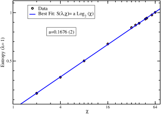
We can now match this scaling to the result of Ref.[10] that states that, away from criticality, $S\simeq\frac{c}{6}\log\xi$. Then, the hypothesis of finite-$\chi$ scaling suggests the half-chain entropy to behave as

$$S_{\chi}\sim\frac{c}{6}\log\chi^{\kappa}.$$ (23)

In the case of the Ising model, we find

$$\xi=\chi^{\kappa},\qquad{\rm with\ }\kappa\simeq 2.011(2),$$ (24)

where we have used that the central charge $c$ is equal to $1/2$ for the Ising model. The error in our result only reflects the quality of the fit. This depends on the use of small values of $\chi$, where scaling may not be present, and on possible violations of that scaling. The uncertainty is then not representing a faithful systematic error but just the order of magnitude of the freedom in the fit. Our goal in this paper remains to collect a first consistent estimate for what is the actual value of $\kappa$.

In practical terms, this result shows that numerical exploration of the critical properties should be well described using relatively small MPS. A value of $\chi\sim 20$ describes faithfully correlations up to 400 sites.

We now consolidate this result by checking its consistency with the computation of other observables.

III.2 Shift of the critical point

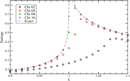
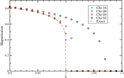
In the vicinity of the critical value $\lambda^{*}=1$, the entanglement entropy of half of the Ising chain diverges and the magnetization abruptly drops to zero. The best MPS approximation to this scenario manages to produce a peak in the entropy and sudden drop of the magnetization for values of $\lambda$ which are shifted from the infinite chain critical value. We label $\lambda^{*}_{\chi,S}$ the coupling where the entropy presents a peak and the $\lambda^{*}_{\chi,M}$ the one where the magnetization vanishes abruptly. As in finite size simulation schemes [11], we have found that both $\lambda^{*}_{\chi,S}\neq\lambda^{*}$ and $\lambda^{*}_{\chi,M}\neq\lambda^{*}$. But we have found that, within the accuracy of our simulation, $\lambda^{*}_{\chi,M}=\lambda^{*}_{\chi,S}=\lambda^{*}_{\chi}$. This can be understood as a check of the consistent representation of criticality that MPS develop.

Our results are shown in Fig. 2 for the entropy and the magnetization respectively. We can see that (i) the amplitude of the shift $\lambda^{*}-\lambda^{*}_{\chi}$ reduces when we increase $\chi$, (ii) the peak of the entropy rises with increasing $\chi$, and that (iii) far from the critical point, modest values of $\chi$ are sufficient to get faithful approximation of the ground state (in the sense that the curves obtained for different values of $\chi$ tend to collapse).

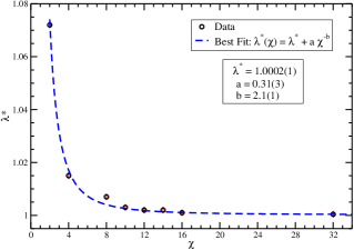
We have checked that the shift of the critical point obeys the law (13). The results are plotted in Fig. 3. As expected, the way $\lambda^{*}_{\chi}$ approaches $\lambda^{*}$ is correctly described by a power law. Using $\nu=1$ we extract:

$$\kappa=2.1(1)$$ (25)

where, again, the error is only reflecting the precision of the fit.

This value is compatible with the value extracted using the entanglement entropy. We see, however, that this estimation is less precise. This fact is related to the difficulties encountered in the determination of $\lambda^{*}_{\chi}$. In principle the finer the scan, the more precise the value of $\lambda^{*}_{\chi}$. However the sharpness of the scan is limited by the numerical precision with which we obtain the entropy. At some point, entropies of chains with close but different values of $\lambda$ are compatible within their error bars. Then, we cannot further refine our scan and should accept the obtained precision as the best we can achieve for the location of the transition.

Figure 2: Entropy and magnetization around the theoretical critical point obtained for $\chi=2,4,8$ and $16$ using, as described in the appendices, $\varepsilon=10^{-1}$ and after convergence of the eighth decimal. The error bars due to the finite value of $\varepsilon$ are smaller than the points size.

Figure 3: Effective critical point $\lambda^{*}_{\chi}$ as a function of $\chi$. As discussed in the appendices, the values for $\chi=2$ and $4$ were obtained with $\varepsilon=10^{-3}$, while for $\chi=8$, $16$ and $32$ with $\varepsilon=10^{-2}$. The errors bar are due to the finite value of $\varepsilon$.

III.3 Magnetization

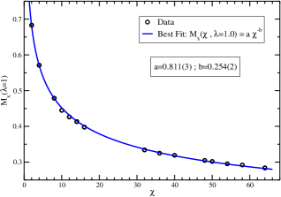
The drop of the magnetization near the critical point obeys scaling laws as discussed previously. We actually expect the magnetization at finite $\chi$ to behave as $M_{\chi}(\lambda=\lambda^{*})\sim\chi^{-\frac{\beta\kappa}{\nu}}$ with the Ising critical exponents $\beta=1/8$ and $\nu=1$. We may now take our numerical results and fit $\kappa$ in this expected scaling law. In Fig. 4, we have plotted $M_{\chi}$ as a function of $\chi$ for the Ising chain at $\lambda=1$. By fitting our numerical results with a function of the form $a\chi^{b}$ (see Fig. 4), we obtain:

$$\kappa=2.03(2).$$ (26)

This value of $\kappa$ is in agreement with our two previous determinations.

Figure 4: Magnetization as a function of $\chi$ at $\lambda=1$.

III.4 Block entropy

A new consistency check consists in considering the entropy of the reduced density operator of a block of $L$ contiguous particles. For a critical systems, this entropy scales with $L$ as $S_{L}\simeq\frac{c}{3}\log L$ [8]. We have observed that, for a fixed value of $\chi$, this entropy saturates at a distance $L\simeq\chi^{\kappa}$. We can make a very qualitative assumption on the fact that the length at which the entropy saturate is of the order of the correlation length and in this way use this value as determination of the correlation length. It is likely that this qualitative assumption can be made rigorous in a renormalization group framework by introducing a new scaling field $\chi^{\kappa/\nu}$. However this analysis is out of the scope of this paper. By using the relation (10) with this estimation of the correlation length we can have an idea of the magnitude of $\kappa$.

In order to compute the entropy of a block of $L$ spins, we have used the ideas contained in the work by Verstraete et al. [17]. The basic idea is to reconstruct the effective new matrix MPS upon successive RG coarse-graining transformations. Our results are displayed on Table 1, where we can see that $S_{L}$ saturates for $L\simeq\chi^{2}$. So that we get a further confirmation that, for the Ising model,

$$\kappa\sim 2.0(1),$$ (27)

in agreement with the previous estimations, though less accurate. We observe that for sufficiently large $L$, $S_{L}$ is approximately equal to two times $S_{\chi}$ (the half-chain von Neumann entropy) calculated at the same $\lambda$. Let us recall that the explanation for this factor $2$ is that a finite block has two boundaries available to establish correlations with the rest of the chain, whereas a half-infinite chain only has one.

$L$	$S(L,\chi=2)$	$S(L,\chi=4)$	$S(L,\chi=8)$
2	0.2994	0.4825	0.5883
4	0.3279	0.5647	0.6976
8	0.3317	0.6271	0.7934
16	0.3317	0.6586	0.8720
32	0.3317	0.6586	0.9288
64	0.3317	0.6586	0.9577
128	0.3317	0.6586	0.9630
256	0.3317	0.6586	0.9632
512	0.3317	0.6586	0.9632
1024	0.3317	0.6586	0.9632

Table 1: Entropy of a block of $L$ spins using the ideas contained in [17]. We observe that the entropy saturates around $L\sim\chi^{2}$. Note that the values obtained for the entropy after saturation are the double of those obtained for half of the chain. This factor of two is due to the fact that here the block has two boundaries.

III.5 Correlation length

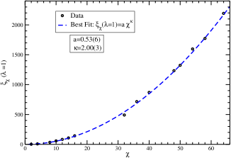
All our previous results should be a consequence of the emergence of a finite correlation length $\xi_{\chi}$. This fact was first investigated in Ref. [9]. We can address this point by analyzing the ratio of the two highest eigenvalues of the transfer matrix [16] computed from the matrices in the MPS. On Fig.(5), we have plotted the value of $\xi_{\chi}$ as a function of $\chi$. To extract the value of the exponent $\kappa$, we have performed a fit to numerical data with a function of the type $a\chi^{\kappa}$ with $a$ and $\kappa$ left as free parameters. We have found

$$\kappa=2.00(3).$$ (28)

Again, the consistency of this result with our previous determinations is manifest.

Figure 5: Correlation length as a function of the size of the $\chi$ in the case of the Ising model at $\lambda=1$.

III.6 Scaling function for the magnetization

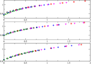
A further manner to test finite-$\chi$ scaling is to analyze in more detail the magnetization. It follows from the scaling analysis in Sect. II that $M_{\chi}$ depends on $\chi$ only through the product $x=\chi^{\kappa/\nu}t$. Therefore, we can plot the rescaled magnetization $M_{\chi}(\chi^{\kappa/\nu}t)\chi^{\kappa\beta/\nu}$ as a function of $\chi^{\kappa/\nu}t$ for different values of $\chi$, assuming the known values of $\nu=1$ and $\beta=1/8$ of the Ising universality class. In case finite-$\chi$ scaling is verified, all points should lie on the same curve. The quality of this collapse is, hence, a function of the correct value of $\kappa$ alone.

We have scanned $\kappa$ for a broad range of values and selected the ones that qualitatively produced a collapse of the numerical points onto a single curve. Remarkably, we have verified that only for a relatively small interval of $\kappa$ values, all the points obtained with this procedure lie on the same curve. Whatever small variation outside this interval of $\kappa$ reflects on a sensible spread of the point outside the curve.

Our results are displayed on Fig.6. Again, we find a further confirmation that $\kappa\simeq 2.0(1)$ is the right scaling exponent.

Figure 6: Collapse of the rescaled magnetization obtained with different MPS using distinct values of $\kappa$ on the scaling function: $\kappa=1.9,2.0,2.1$ for upper, middle and lower graphs, respectively.

III.7 Scaling function for the the energy difference and comparison with classical results

In this section, we clarify why studying the deviation from the critical point with finite MPS we face a two scale problem. This problem is the quantum version of the already studied two scale finite-size scaling ansatz in the context of classical systems [19]. In our case, the analysis is performed considering infinite size systems.The first scale is given by the MPS dimension $\chi$ and the second scale is given by $t$. We saw in the previous section that by correctly treating the two scales, one is able to extract universal scaling functions. The universality, implies that scaling functions however, should not depend on which system, among those in the same universality class, one decide to consider. This statemet can be checked by comparing our results with the one contained in Ref. [19] about the classical Ising model in two dimensions at critical temperature. This system is indeed in the same universality class we are considering: the two dimensional Ising universality class. The authors apply the ideas of the Corner Transfer Matrix (CTM) renormalization group [20] to it. This is a technique that generalizes the DMRG renormalization ideas and its related variational techniques over MPS to a real space renormalization algorithm for classical systems. Once the CTMRG is applied at critical temperature as in ref. [19] a new scale emerges. This is the inverse of a correlation length depending on the dimension of the renormalized CTM $m$. The authors label this scale $\xi(m)$. This scale exactly corresponds to the scale we are calling here $\xi_{\chi}$ . In this way, the authors of ref. [19], by treating the finite size classical system of dimension $N$ studied with a finite renormalized CTM of dimension $m$ as a two scale problem, extract the value of all critical exponents. Here we consider the precise map between our results and the one contained there. Following the recipes in Ref. [20] we see that, (as already implicit in the identification of scales) the classical correspondence of $\chi$ is the size of the renormalized CTM (called $m$ in both references). We can use again the finite size scaling ansatz and map the distance from the critical point that we call $t$ to the size of the classical system considered in ref. [19] ( called $N$ ). In this way the scaling variable $x_{m}=\xi(m)/N$ of ref. [19] is related to the one we use $x$ as : $x_{m}=x^{\nu}$. As for the Ising model $\nu=1$, the results in ref. [19] should exactly correspond to ours. We check this claim by consider what in our language would be the plot in figure 3 of Ref. [19]. It represent the energy difference as a function of $x$ with respect to the exact result. We can use the standard mapping between the free energy of a classical system and the ground state energy of the corresponding quantum system and compare the plot in figure 3 of ref. [19]. with our results for the ground state energy per bond. To do this we plot the difference of the ground state energy with a given $\chi$ and the exact result $E(\infty)=-1.27323954$. The scaling function for the energy difference is obtained by plotting $(E_{\chi}(1/x)-E_{\infty})\chi^{\kappa/\nu}$ . Again we see that by using a value of $\kappa=2$ the points obtained with different $\chi$ collapse to a single curve. We also see that the curve we obtain has the same shape but a different normalization factor with respect to the one obtained in figure 3 of Ref. [19]. This is expected since the normalization factors are known to be universal but boundary condition dependent [21] and we used different boundary condition from the ones used in Ref. [19].

Figure 7: Collapse of the rescaled energy difference obtained with different MPS. The values we use are $\kappa=2$, $E(\infty)=-1.27323954$.

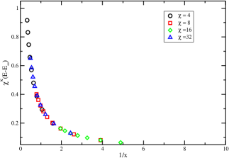
We can hence confirm that the scaling observed in this work in the case of a quantum phase transition is the analogue to the one observed in a classical phase transition in ref. [19].

IV Evidence of finite-$\chi$ scaling for the Heisenberg chain

An extensive analysis of the emergence of finite-$\chi$ scaling in different models is necessary to gain insight in the role of the scaling exponent $\kappa$. Here, we only make a first step and explore the Heisenberg spin 1/2 Hamiltonian

$$H=\sum_{i}\vec{\sigma}_{i}\cdot\vec{\sigma}_{i+1}\ .$$ (29)

We may conjecture that $\kappa$ should only vary with the universality class of the model considered. To assess the new value of $\kappa$, we consider the scaling of the half chain entropy since this strategy provided very precise determination in the Ising case.

We then follow the same steps as described for the Ising case and we take the central charge to be $c=1$. By fitting the numerical data with a curve of the type $a+b\log\chi$ and using the actual value of the central charge we obtain, as observed on Fig. 8,

$$\kappa=1.36(2).$$ (30)

Let us note that the fit now includes a non-zero intersect. This was absent in the Ising case.

This result can be checked for consistency in a similar way as the results presented for the Ising model. Here, we present as a further piece of evidence for finte-$\chi$ scaling the scaling of the correlation length as computed from the ratio of the largest eigenvalues of the transfer matrix. As shown in Fig. 9, the numerical data are described correctly by a law of the type in Eq. (10) with an exponent

$$\kappa=1.38(2).$$ (31)

Figure 8: Entropy as a function of $\log\chi$ for the Heisenberg model. Data have been fitted with a function of the type $a+b\log(\chi)$ with $a$ and $b$ free parameters. The results of the factor $b$ for the fit in the $\chi$ interval from $16$ to $44$ is $b=0.226(2)$.

Figure 9: Correlation length as a function of $\chi$ in the case of the Heisenberg model. This behavior can be correctly described by a relation of the type 10 with an exponent $\kappa=1.38(4)$. The fit has been performed in the $\chi$ interval $20-44$

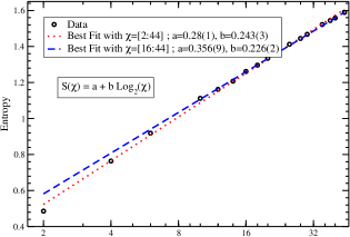
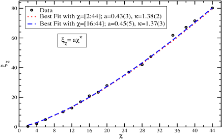
Both determinations in Eq. (30) and (31) are compatible and support the value $\kappa\sim 1.37(2)$, which depends on the universality class of the model under discussion.

V Applications of finite-$\chi$ scaling

As in the case of finite size scaling, we can use finite $\chi$-scaling to extract critical exponents. The ideal strategy is the one that does not rely on the knowledge of the position of the finite $\chi$ pseudo critical point. This is so because the determination of the pseudo critical point is very delicate. Any small error in it propagates to the determination of critical exponents as we explicitly saw when dealing with the determination of $\kappa$.

Keeping this in mind, we can envisage two different scenarios: a first simple scenario, as the one of the Ising model, when we know a priori the location of the phase transition. In this case, in order to extract the critical exponents we proceed as follows: i)Extract the value of $\kappa$ by studying the behavior of $\xi_{\chi}$ at the critical point. ii) Extract all the ratios $\alpha/\nu$ where here $\alpha$ represents a generic critical exponent by studying universal quantities as function of $\chi$ at the phase transition using the value of $\kappa$ obtained in i). iii) Extract the value of $\nu$ (and hence $\alpha$ from the ratio obtained in ii) )by studying the derivatives of the universal quantities with respect to $t$. The second scenario and by far the most unfavorable and frequent is the one where we do not know the location of the critical point. In this case, we need to adapt some strategy known from finite size analysis to extract its value if we want to apply finite $\chi$-scaling to the transition. A possibility is obtained by considering the techniques of [22] (more efficient methods can be found i.e. in Ref. [23, 24]). A review of this method for the case of finite size scaling is contained in ref. [25]. We adapt it in the following way: we iteratively obtain estimates of $\kappa$ and the critical point by considering the behavior of the correlation length as a function of increasingly big $\chi$. Once these estimates converge to a fixed value, we can use the obtained values for $\kappa$ and for the critical point to repeat the steps from i) to iii) of case one. In this way we extract all the other critical exponents. The main source of error in all these determinations is, as in the case of the finite size scaling, the existence of scaling violations that we do not analyze in this work. However, even without taking the scaling violations into account, we think that the extracted exponent should be much more accurate than the ones obtained with standard techniques. To justify this statement, we review what we mean by standard techniques for extracting critical exponents with an infinite MPS by considering again the case of the Ising model.

We can extract the value of the exponent $\nu$ by studying the behavior of the correlation length at fixed $\chi$ when we approach the phase transition. We expect that far enough from the region where finite-$\chi$ effects appear, a modest value of $\chi$ should provide a faithful description of the Ising ground state. The correlation length should obey a law of the type $(\lambda-\lambda^{*})^{-\nu}$. Fitting the data with this function and leaving $\lambda^{*}$ and $\nu$ as free parameters we obtain an estimate of both $\lambda^{*}$ (the phase transition point) and $\nu$. We also expect that due to systematic errors induced by the fitting procedure (the difficult point is to locate the correct window of $\lambda$ values for which we should perform the fit) these estimates would have a slight dependence on $\chi$ and should converge to the exact $\lambda^{*}$ and $\nu$ for $\chi$ large enough. In Fig. 10 we show the results of such study, again for the Ising model. We extract as best estimate of $\nu$ in the case of $\chi=16$

$$\nu\simeq 1.00(5).$$ (32)

See also Ref. [26, 19, 27] and references therein to see how in the case of finite chains described with MPS, finite size scaling can be used as an alternative to extract critical exponents .

Figure 10: Fine tuning of the correlation length around the critical point for $\chi=16$ and $\varepsilon=0.1$. Note that the points are not equally spaced. Inset: Values obtained for $\nu$ by fitting magnetic field window of different sizes (all starting at $\lambda=0.90$ and finishing at the point in the x-axis). We notice a good region of stability which can be used to extract our best estimate for the $\nu$ exponent.

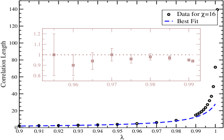
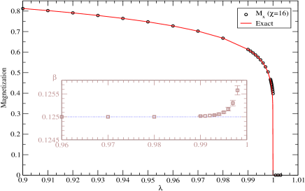
A similar strategy can be used to extract the $\beta$ critical exponent. Again, working slightly away from criticality, the scaling of the magnetization is very nicely fitted with

$$\beta\simeq.1250(1)$$ (33)

as shown in Fig. 11.

Figure 11: Fine tuning of the magnetization around the critical point for $\chi=16$ and $\varepsilon=0.1$. Note that the points are not equally spaced. Inset: Values obtained for $\beta$ by fitting magnetic field window of different sizes all starting at $\lambda=0.90$. We clearly notice a good region of stability which can be used to extract our best estimate for the $\beta$ exponent.

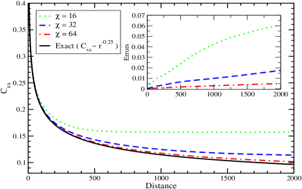
In addition to the exponent $\beta$, one can consider the exponent $\eta$ by studying the behavior of the two point correlation function of the order parameter $\sigma_{x}$. Both exponent are related via the hyper scaling relation: $\beta=(d-2+\eta)/2$, where in this case $d=2$ as we are considering the universality class of the classical two dimensional Ising model.

This relation implies that if $\beta=1/8$, then $\eta$ should be $1/4$. We checked this for consistency. We plot the two point correlation function of the order parameter as a function of the distance in Fig. 12. In a log-log plot, an algebraic decay such $r^{-\eta}$ is seen as a straight line. We plot this straight lines together with the correlations functions obtained for the MPS at the phase transition with $\chi=16,32,64$. We appreciate how the range for which the correlations reproduce the exact result increases with the matrix dimension. Once the range of distances is correctly selected, a fit to a power law in the case of correlation function of the $\chi=64$ MPS at $\lambda=1$ produce the following best estimate for $\eta$

$$\eta\simeq.24800(25).$$ (34)

Again, this result only reflects the quality of the fitting strategy.

Figure 12: Study of the order parameter two point correlation function at $\lambda=1$ for $\chi=16,32,64$ and $\varepsilon=0.01$ compared with the expected exact behavior $r^{-0.25}$. We note that the range of distances for which there is good agreement between the numerical correlation function and the exact result increases with $\chi$ as expected. Inset: Results of fits with a power law of the type $ar^{-\eta}$ for the case of $\chi=64$ in the $r$ windows for which the extracted correlation functions agree with the analytical results.

VI Conclusions

The amount of entanglement supported by the MPS approximation is limited by the size $\chi$ of the matrices that form the ansatz. We have studied numerically this issue and found that all observables we have considered approach their exact values at criticality obeying scaling laws in $\chi$. The case of the quantum Ising chain in a transverse field is consistently described by an effective finite correlation length that scales as $\xi_{\chi}=\chi^{\kappa}$, with $\kappa\simeq 2$. Most of the results presented here were related to the Ising model, but the numerical work we have performed shows that our findings are qualitatively valid for other models, such as the Heisenberg model where our calculations indicate that $\kappa\simeq 1.36$. Interestingly, the value of $\kappa$ seems to be model-dependent.

In the case of the Ising model, it is specially interesting to note the accurate fit of the half-chain entropy to $S\sim\frac{1}{6}\log\chi$ at $\lambda=1$ with no constant or important subleading corrections. This effect is not present for the Heisenberg model.

All our numerical results were found using the iTEBD algorithm and checked to agree with standard DMRG [6, 28]. It would be, in principle, possible to use other algorithms as a brute force minimization of energy in the space of matrices in the MPS structure. Such an approach may fail due to the proliferation of local minima. Somehow, DMRG and iTEBD manage to circumnavigate local minima an find the absolute minimum within the approximation.

We have also checked that the scaling we encounter here coincides with the emergence of a second scale in some treatment of classical phase transition as pointed out in Ref. [19].

This correspondence is a hint that this phenomenon is quite general and appears whenever one tries to approximate operators with an infinite rank (such as the CTM or the half chain reduced density matrix) with finite rank operators Therefore it is likely that scaling is not strictly related to the MPS representation of the ground state. We are currently investigating this issue by repeating a similar study to the one presented here with different tensor network representations [29].

With the same reasoning, we expect finite-$\chi$ scaling to appear for some generalizations of MPS, such as Tensor Product States [30] also known as Projected Entangled Pairs States [31]. It remains an open problem to derive the scaling relation analytically for exactly solvable models.

VII Acknowledgments

We thank P. Calabrese, J. I. Cirac, J. J. García-Ripoll, Ll. Masanes, S. Montangero, R. Orús, M. Roncaglia, E. Vicari and G. Vidal for discussions and suggestions on the topics presented here. We thank I. P. McCulloch for his comments on the manuscript. Financial support from QAP (EU), MEC (Spain), Generalitat de Catalunya and CAPES (Brazil) is acknowledged.

Appendix A Error control and convergence issues with the iTEBD algorithm

In this section, we wish to address the reliability of the data output by the iTEBD algorithm. Let us start by reminding the main features of this algorithm. A more technical presentation can be found in [12].

The iTEBD algorithm aims at finding the ground state energy per particle of a Hamiltonian of the form

$$H=\sum_{i=-\infty}^{\infty}h_{i},$$ (35)

where $h_{i}$ represents a two-spin next-neighbor interaction term. This algorithm is based on the following identity, valid for any gapped Hamiltonian:

$$|\Psi_{g}\rangle=\mathcal{N}\lim_{\tau\to\infty}e^{-\tau H}|\Psi_{0}\rangle.$$ (36)

That is, a ground state of $H$ can be obtained by evolving some initial state $\Psi_{0}$ in imaginary (Euclidean) time whenever $H$ has a gap above the ground state and $\langle\Psi_{0}|\Psi_{g}\rangle\neq 0$. For many Hamiltonians of interest, though, Eq.(36) cannot be used as such. Rather, one computes the following sequence until convergence is attained:

$$\Psi_{i+1}=\mathscr{E}_{i}(\epsilon,H)\Psi_{i}/||\mathscr{E}_{i}(\epsilon,H)\Psi_{i}||,$$ (37)

where $\epsilon$ is some tunable parameter such that $\mathscr{E}_{i}(\epsilon)\simeq e^{-\epsilon H}$ for $\epsilon$ small enough. In the iTEBD algorithm, $\mathscr{E}_{i}(\epsilon,H)$ is decomposed into

$$\mathscr{E}_{i}(\epsilon,H)=\mathscr{Q}_{i}\mathscr{P}_{i}\mathscr{F}_{i}(\epsilon,H),$$ (38)

where the factors appearing in the last expression correspond each to a different approximation that makes numerical computations tractable:

• i) The first factor $\mathscr{F}_{i}(\epsilon,H)$ comes from using a cut off Suzuki-Trotter expansion [1] in order to approximate the action of $e^{-\epsilon H}$ by a product of two-body operators. (As a result, the form of $\mathscr{F}_{i}$ depends on $i$.) The error introduced by truncating the Suzuki-Trotter expansion vanishes when $\epsilon\to 0$. We call this error finite time step error.

• ii) The second factor $\mathscr{P}_{i}$ is a projector that approximates $\mathscr{F}_{i}(\epsilon,H)\Psi_{i}$ by an MPS with matrices of some prescribed finite size $\chi$. This approximation is made in order to have an efficient description of the state at each step of the sequence (37). Indeed, both storing of $\Psi_{i+1}$ and the computation of the mean value of a local operator now takes a time that is polynomial in $\chi$ [12]. This approximation boils down to limiting the amount of correlations present in the system. We will call truncation error the error due to this approximation.

• iii) The operator $e^{-\epsilon H}$ is not unitary, and as a result $\mathscr{P}_{i}\mathscr{F}_{i}(\epsilon,H)$ neither is. This non-unitarity have small spurious effects that we can safely neglect . The third operator, $\mathscr{Q}_{i}$, does exactly this job, producing what we call an orthonormalization error.

In order to study the time-step error, we have applied the iTEBD algorithm to obtain an MPS approximation of the ground state of the quantum Ising chain with matrices of size $\chi$ equal to 2. The reason why we have chosen to discuss the time-step error with such a small value of $\chi$ is that it is most illustrative. For various values of $\epsilon$ ranging from $10^{-1}$ to $10^{-5}$, we have computed the behavior of the ground state energy and the half-chain von Neumann entropy. It is natural to test the performance of the algorithm looking at the ground state energy since it is designed to minimize this quantity. It is less obvious why we also looked at the half-chain entropy. We will explain it shortly.

In principle, the smaller $\epsilon$, the more accurate the description of the state. But small values of $\epsilon$ also increase the number of time steps necessary to guarantee convergence of the simulation. One way to proceed, in order to correctly choose $\epsilon$, is as follows: (i) run a simulation with a rather large value of $\epsilon$, $\epsilon_{1}$, and get an estimate of the energy and the entropy. (ii) Repeat the simulation with a smaller value of $\epsilon$, $\epsilon_{2}$, and compare the resulting energy and entropy with those of the simulation at $\epsilon_{1}$. (iii) If the results are close enough (according to a predetermined margin), stop the simulation. Otherwise, repeat with smaller values of $\epsilon$ until convergence is attained.

$\lambda$	S1-S5	S2-S5	S3-S5	S4-S5
0.9	9124	921	91	8
1.0	42495	4203	416	38
1.071	368647	35489	3501	318
1.072	69632	6951	689	62
1.073	69200	6908	684	62
1.1	58718	5871	581	53

Table 2: Convergence of the entropy as a function of $\varepsilon$ for some values of $\lambda$. The table shows the difference of the entropy found using a given $\varepsilon$ with our best simulations corresponding to $\varepsilon=10^{-5}$ ( S1 is the value of the half-chain entropy obtained for $\varepsilon=10^{-1}$, S2 the values obtained for $\varepsilon=10^{-2}$ and so on). All entries in this table should be multiplied by $10^{-8}$.

$\lambda$	$\Delta E$	$\Delta S$
0.5	$<0.1$	39
0.7	$<0.1$	706
0.8	$<0.1$	2521
1.0	7	42495
1.071	41	368647
1.072	34	69632
1.073	34	69200
1.1	29	58718
1.4	7	14226
1.5	4	9807

Table 3: $\Delta E$ and $\Delta S$ corresponding to the difference between the values obtained for the entropy and energy when using $\varepsilon=10^{-1}$ and $\varepsilon=10^{-5}$ for $\chi=2$. This gives an estimation of the error due to $\varepsilon$ when using $10^{-1}$ as its value. Note that the errors increase around the critical point and that the errors in the entropy are much greater than the ones in the energy. All entries of this table should be multiplied by $10^{-8}$.

On Table 2, we report on the convergence of the von Neumann entropy, as a function of $\epsilon$, for various values of $\lambda$, while Table 3 shows the difference of the values for the energy (resp. entropy) for $\epsilon=0.1$ and $\epsilon=10^{-5}$. We interpret these differences as an estimation of the finite time step error at $\epsilon$. (The results for the energy with $\epsilon=0.1$ and $\epsilon=0.01$ are already identical up to 8 decimals. This is why we have not shown them.) We observe from these tables that the error on the entropy is about ten times larger than that on the energy and that both increase around the pseudo critical point $\lambda_{\chi}^{*}$. Simulations with $\chi=4$ and $\chi=8$ show similar results. If we now compare the values of the energy and entropy yielded by our simulations with the exact values for an infinite chain (Table 4 and Table 5), we see that the errors are larger in the vicinity of the critical point and that, as expected, they decrease as we decrease $\epsilon$.

$\lambda$	Exact	$\chi=2$	$\chi=4$	$\chi=8$	$\chi=16$
0.5	1.06354440	33	$<0.1$	$<0.1$	$<0.1$
0.6	1.09223858	172	$<0.1$	$<0.1$	$<0.1$
0.7	1.12682867	745	2	$<0.1$	$<0.1$
0.8	1.16780951	2978	12	$<0.1$	$<0.1$
0.9	1.21600091	12173	126	$<0.1$	$<0.1$
1.0	1.27323954	69712	4683	261	15
1.1	1.34286402	146576	1642	6	$<0.1$
1.2	1.41961927	77696	416	$<0.1$	$<0.1$
1.3	1.50082324	45675	141	$<0.1$	$<0.1$
1.4	1.58518830	28719	57	$<0.1$	$<0.1$
1.5	1.67192622	18964	25	$<0.1$	$<0.1$

Table 4: Errors in the energy in relation to the exact value for $\chi=2,4,8\mbox{ and }16$. These errors are greater around the critical point (which for $\chi=2$ is close to $\lambda=1.1$). These values were obtained with $\varepsilon=0.1$, showing a clear dominance of truncation error over the errors introduced by finite step time evolution. All entries of this table should be multiplied by $10^{-8}$.

$\lambda$	Exact	$\chi=2$	$\chi=4$	$\chi=8$	$\chi=16$
0.5	421292	-3	-3	$<0.1$	$<0.1$
0.6	914778	-36	-36	$<0.1$	$<0.1$
0.7	1869961	-389	-389	$<0.1$	$<0.1$
0.8	3804448	-4255	-4255	-1	$<0.1$
0.9	8484551	-66920	-66920	-12	-2
1.1	47444179	-437545	-437545	-6473	-3
1.2	36551466	-74387	-74387	-270	5
1.3	30064632	-20221	-20221	-23	5
1.4	25539496	-6976	-6976	$<0.1$	5
1.5	22144107	-2797	-2797	4	5

Table 5: Errors in the entropy for different values non-critical $\lambda$ and of $\chi$. All values have been multiplied by $10^{8}$. Note the increasing accuracy as a function of $\chi$.

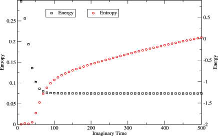
Let us now clarify why we were interested in reaching full convergence for the half-chain entropy. A common method to locate a phase transition is to analyze the variation of an order parameter. On another hand, we know that the half-chain entropy of a critical system diverges while, off and close to criticality, it scales as the logarithm of the correlation length and thus remains finite [8]. It is therefore reasonable to think of using the half-chain von Neumann entropy, to detect a phase transition. It turns out that when running the iTEBD algorithm, $S$ converges faster to a steady value than the mean value of the order parameter and thus provides a faster detection of the position of the critical point (varying the magnetic field, $\lambda$, and scanning for the peak of $S$). Yet, the von Neumann entropy converges more slowly than the energy, see Fig. 13. Around the critical point, the spectrum of the Hamiltonian is filled with a lot of low-energy excited levels which energy is very close to that of the ground state. An arbitrary superposition of such excited states will have energy close to that of the ground state, but can in principle exhibit very different entanglement properties. We believe that this is why it takes much longer to get a reliable estimate of the entropy. One has to make the energy converge close enough to that of the ground state so that the entropy of the obtained state also faithfully reflects that of the ground state.

Figure 13: Convergence of the energy and entropy, at the effective critical point, during the imaginary time evolution, with $\chi=8$, $\lambda=1.006$ and $\varepsilon=10^{-2}$. The full convergence of the energy (eight decimals) took $\sim 10^{5}$ steps while $\sim 6\ 10^{5}$ steps where necessary to make the entropy converge.

Appendix B Metastabilities

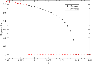
An important issue when running the iTEBD algorithm is to be sure that one is not driven to a local minimum. Here we point out the existence of some meta stabilities in the simulation with respect to the choice of the initial state (an effect which is also present in standard DMRG simulations). In all our calculations, we have used an initial state which matrices $\Gamma_{A}$ and $\Gamma_{B}$ (see [12] for details) are of the following form : random entries in the $2\times 2$ left upper corner, and all other entries set to zero. However, when performing a simulation for the Ising chain for some value $\lambda$ of the transverse field, one could use, as initial state, the result of a simulation performed at some close value of $\lambda$. Although this procedure can substantially decrease the time necessary to make the energy and the half-chain entropy converge, it can also lead to misleading results regarding the position of $\lambda^{*}_{\chi}$, taken as the point where the order parameter vanishes, as can be seen on Fig. 14. Simulations which start from a previous minimization run of a larger $\lambda$ do produce unphysical results. Thus, all simulations must start from random initial conditions.

Figure 14: Magnetization as a function of the transverse magnetic field using different initial states for $\chi=4$ and $\varepsilon=0.1$. In one case (open circles) we use a random $2\times 2$ matrix as an initial state. In the second case (open squares) the initial state for $\lambda=\lambda_{0}$ is the final state obtained for $\lambda=\lambda_{0}+0.001$. The two methods do not give similar results for the position of the critical point.

Appendix C Boosted iTEBD

The performance of the iTEBD algorithm depends on the initial conditions and the gap above the ground state. The results of our study suggest that using finite $\chi$ one is perturbing the system in a way similar to have an effective gapped Hamiltonian. However, if the gap is small the convergence of the algorithm can be very slow. To see this, we can consider as initial state a state with non zero projection on the ground state

$$|\psi\rangle=\alpha|\psi_{0}\rangle+\sqrt{(1-\alpha^{2})}|\psi_{\perp}\rangle$$ (39)

with $|\alpha|<1$. It is easy to see that, if the Hamiltonian has a gap $\Delta$, the Euclidean evolution of an initial state with non zero projection on the ground state will lead to:

$$|\psi^{\prime}\rangle=\exp(-H\tau)|\psi\rangle=\alpha\exp(-E_{0}\tau)|\psi_{0}\rangle+\sqrt{(1-\alpha^{2})}|\psi^{\prime}_{\perp}\rangle$$ (40)

with $|\psi^{\prime}_{\perp}\rangle=\exp(-Ht)|\psi_{\perp}\rangle$. From

$$\langle\psi^{\prime}_{\perp}|H|\psi^{\prime}_{\perp}\rangle\geqslant\Delta+E_{0},$$ (41)

we see the long time limit of the above expression, differs from the ground state (as already pointed out in ref. [1]) by terms of the order:

$$|\langle\psi_{0}|\psi^{\prime}\rangle|\sim 1-\frac{1-\alpha^{2}}{2\alpha^{2}}\exp(-2\tau\Delta).$$ (42)

Now if we approach the critical point of a phase transition we know that the correlation length scales with the critical index $\nu$ of the corresponding universality class

$$\xi\sim t^{-\nu},$$ (43)

where $t$ denotes, again, the distance from the critical point. Assuming that $\Delta\sim 1/\xi$, we see that, even in the case of a good guess of the initial state (that is, in the case $|\alpha|^{2}\sim 1$), the convergence of the algorithm slows down in the critical region. In order to partially cure this slowing down we can perform a linear extrapolation of the results obtained after a small interval of Euclidean time $d\tau$ and get a new estimate for the MPS. Given a generic element of the MPS matrix at Euclidean time $\tau$, $A(s_{i})(\tau)$, and the same element at time $\tau+d\tau$, $A(s_{i})(\tau+d\tau)$, we construct a new MPS which matrix elements $A(s_{i})(T)$ are the extrapolation at time $T$ of the straight line passing from the two points at $\tau$ and $\tau+d\tau$. Before promoting the guessed MPS to a new initial condition, we should check that the state it describes has a lower energy than the MPS obtained at $\tau+d\tau$ before the extrapolation. A lower energy indeed means a greater overlap with the ground state. In this case the extrapolation is successful and we promote the guess to an initial condition of the new evolution. In case the energy of the new extrapolated state is greater than the energy of the state before the extrapolation, we just neglect it and keep the state we had before the extrapolation. The new Euclidean evolution is also of length $d\tau$ and is followed by the attempt of a new extrapolation. We iterate the procedure till we reach convergence. We call this technique boosted iTEBD.

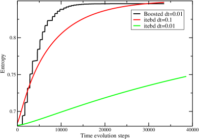
In order for the extrapolation to work, we have to tune finely its two parameters: the waiting time $d\tau$ and the amount of time we extrapolate, $T$. Once these two parameters are fixed, we are able to accelerate the convergence by a factor greater than $10$. A typical case is shown in Fig. 15 where we show the convergence of the simulations of a $\chi=32$ MPS at $\lambda=1$. Without the boosted iTEBD algorithm, with $\varepsilon=0.01$, after the number of Trotter steps considered, the system had still not converged. Increasing $\varepsilon=0.1$ translates in a coarser precision but with a convergence time about ten times shorter. A further improvement in convergence is obtained by keeping the same $\varepsilon=0.01$, and hence the same precision, but boosting the evolution with the extrapolation technique described. We see that the gain in convergence time is bigger by a factor of ten. As we can see, there is a point where the extrapolation fails and the normal evolution is continued. We can also check that before the first extrapolation, the boosted evolution coincides with the unboosted evolution with the same $\varepsilon$.

Figure 15: Boosted itedb algorithm. We plot the half-chain entropy as a function of the Trotter steps for a $\chi=32$ MPS at $\lambda=1$. This is taken as a typical case from a large number of examples with different $\chi$ and magnetic fields that present a similar behavior. We compare the results obtained with $\varepsilon=0.01$ with both boosted and standard iTEBD and the results obtained with $\varepsilon=0.1$ with standard iTEBD. As we can see, the unboosted case with $\varepsilon=0.01$ is far from having converged in the number of Trotter steps considered. On the other hand, the boosted system with $\varepsilon=0.01$ converges (up to 8 decimals) in a smaller amount of time steps than the unboosted algorithm with an $\varepsilon$ ten times bigger. Indeed, the latter simulation has still not converged in the window of Trotter steps shown. The discrepancy in the asymptotic values is due to $\varepsilon$ corrections described in the previous appendices. From this plot, we can safely deduce that the effect of the boost is to reduce the convergence time by a factor greater than $10$ in the case we have analyzed.

Appendix D Comparison with DMRG

In order to ensure that the effects we observe are not artifacts of the algorithm used, we reproduced some of them with a different algorithm. We have chosen to use the open source code for DMRG written by the Pisa group . This program performs an infinite DMRG update of the system by growing it till it reaches a chosen chain length. At this stage, it performs several finite size sweeps through the chain (at least three in our case) in order to compute the reduced density matrix of all possible chain bipartitions and improve the infinite results [32] .

	Energy	Entropy
DMRG N=16284	-1.27321717	0.68557374
iTEBD	-1.27323939	0.68065196
iTEBD - DMRG(N=16384)	-0.00002222	-0.00492178

Table 6: Comparison of DMRG energy and entropy results with the infinite size result produced by iTEBD with $\epsilon=10^{-4}$ and where both methods used $\chi=16$.

We checked the stability of the presented results on the variation of the number of finite size sweeps. In this way, we are sure that the results have converged. We have checked that for a fixed number of level ($m$ in the language of DMRG that corresponds to $\chi$ in this paper), increasing the chain length makes the results converge to those obtained with the algorithm we have used in the paper. It was interesting to see that the DMRG convergence is however quite slow as compared with the boosted iTEBD.

References

- [1] G. Vidal, Phys. Rev. Lett. 91, 147902 (2003). G. Vidal, Phys. Rev. Lett. 93, 040502 (2004).
- [2] S. R. White, Phys. Rev. Lett. 69, 2863 (1992); Phys. Rev. B 48, 10345 (1993).
- [3] U. Schollwoeck, Rev. Mod. Phys. 77, 259 (2005).
- [4] K. Hallberg, Adv. Phys. 55, 477 (2006).
- [5] S. Östlund and S. Rommer, Phys. Rev. Lett. 75, 3537 (1995); S. Rommer and S. Östlund, Phys. Rev. B55, 2164 (1997).
- [6] I. P. McCulloch, J. Stat. Mech. 10, 10014 (2007).
- [7] M. Fannes, B. Nachtergaele, and R. F. Werner, Comm. Math. Phys. 144 (1992); D. Pérez-García, F. Verstraete, M. M. Wolf and J.I. Cirac, Quantum Inf. Comput. 7, 401 (2007).
- [8] G. Vidal, J. I. Latorre, E. Rico and A. Kitaev, Phys. Rev. Lett. 90, 227902 (2003); J. I. Latorre, E. Rico and G. Vidal, Quant. Inf. Comp. 4 48 (2004). C. Holzhey, F. Larsen and F. Wilczek, Nucl. Phys. B 424, 44 (1994).
- [9] M. Andersson, M. Boman and S. Östlund, Phys. Rev. B 59, 10493 (1999).
- [10] P. Calabrese and J. Cardy, Int. J. Quant. Inf. 4, 429 (2006).
- [11] M. N. Barber, Phase Transitions and Critical Phenomena, edited by C. Domb and J. L. Lebowitz, vol. 8, Academic Press (1983).
- [12] G. Vidal, Phys. Rev. Lett. 98, 070201 (2007).
- [13] R. Orús and G. Vidal, arxiv:0711.3960.
- [14] S. Sachdev, Quantum Phase Transitions, Cambridge University Press (1999).
- [15] P. Pfeuty, Annals of Physics 57, 79 (1970).
- [16] M. M. Wolf, G. Ortiz, F. Verstraete and J. I. Cirac, Phys. Rev. Lett. 97, 110403 (2006).
- [17] F. Verstraete, J. I. Cirac, J. I. Latorre, E. Rico and M. M. Wolf, Phys.Rev.Lett. 94, 140601 (2005).
- [18] R. Orús, J. I. Latorre, J. Eisert and M. Cramer, Phys. Rev. A 73, 060303 (2006).
- [19] T. Nishino, K. Okunishi and M. Kikuchi, Phys. Lett. A 213, 69 (1996).
- [20] T. Nishino, K. Okunishi Journal of the Physical Society of Japan 65, 891-894 (1996)
- [21] Privman, Valdimir and Fisher, Michael Phys. Rev. B 30 322–327 (1984).
- [22] M. P. Nightingale, Physica A 83 (1976) 561; Phys. Lett. A 59 (1976) 486.
- [23] L. Campos Venuti, C. Degli Esposti Boschi, M. Roncaglia, and A. Scaramucci, Phys. Rev. A 73, 010303(R) (2006).
- [24] M. Roncaglia, L. Campos Venuti and C. Degli Esposti Boschi Phys. Rev. B 77, 155413 (2008)
- [25] A. Pelissetto and E. Vicari, Phys. Rep. 368 (2002) 549.
- [26] R. Bursill and F. Gode, J. Phys. Cond. Matt. 7, 9765 (1995).
- [27] M. S. L. du Croo de Jongh, J. M. J. van Leeuven, Phys. Rev. B 57, 8494 (1998).
- [28] J. Dukelsky, M. A. Martín-Delgado, T. Nishino and G. Sierra, Europhys. Lett. 43, 457 (1998).
- [29] J.I. Latorre, V. Pico, L. Tagliacozzo, G. Vidal in preparation
- [30] T. Nishino, K. Okunishi, Y. Hieida, N. Maeshima and Y. Akutsu, Nucl. Phys. B575, 504 (2000).
- [31] F. Verstraete and J. I. Cirac, arXiv:cond-mat/0407066. V. Murg, F. Verstraete and J. I. Cirac, Phys. Rev. A 75, 033605 (2007). G. Vidal, arXiv:0707.1454. J. Jordan, R. Orús, G. Vidal, F. Verstraete, J. I. Cirac, arXiv:cond-mat/0703788.
- [32] G. De Chiara, M. Rizzi, D. Rossini and S. Montangero, cond-mat/0603842