The Network of Commuters in London

Abstract

We study the directed and weighted network in which the wards of London are vertices and two vertices are connected whenever there is at least one person commuting to work from a ward to another. Remarkably the in-strength and in-degree distribution tail is a power law with exponent around $-2$, while the out-strength and out-degree distribution tail is exponential. We propose a simple square lattice model to explain the observed empirical behaviour.

I Introduction.

Applications of graph theory to the study of urban development has a long history, initiated by Euler’s study of urban traffic problems e1 ; e2 . A review of the state of the art on cities and complexity, studied through cellular automata, agent-based models and fractals can be found in b . Following the seminal work of Barabasi et al. on growing scale free networks 4 , many attempts have been made to embed growing networks in a Euclidean bi-dimensional spaceh . Some of these consider vertices to be random points in a selected spacem , some others consider vertices to be cells in a given latticer ; y . Moreover spectral analysis on urban networks v have shown to unreveal many interesting aspects of metropolitan organisation.

We study the network of commuters in London. Data on commuters’ behaviour was obtained from the London 2001 census that is available in lc . London is composed of 634 wards. We consider the network in which vertices are wards and two vertices are linked whenever there is a flux of people commuting from a ward to another to work. Loops are considered. Since this network is embedded in a geographical space we need to introduce a definition of physical distance between the vertices. In a city like London the Euclidean distance is not the best choice if we want to deal with the organization of people and the development of the city. Many places in the city can be very close in terms of Euclidean distance, but far apart if we consider their accessibility, that is the time a person would take to commute from one place to another. For this reason we adopt as a distance between two wards the $generalised$ $time$ $t^{*}$ to travel from a ward to the other. The definition and data sets for the generalised time were developed by Transport for London tfl for the Greater London Authority. The generalised time is defined as $t^{*}=in-vehicle$ $time+2*(waiting$ $time)+1.5*(access$ $and$ $egress$ $time)+interchange+$ $bus$ $boarding$ $penalty$ and it is measured in minutes.

All data available concern just London. For instance people living out of London and working in London, or people living in London and working out of London are not counted. This bias can be important if we consider that the 25$\%$ of people working in the central activity zones of London live out of London.

The links of this network are directed and weighted. The directionality of the network is implicit in the complexity of urban commuting. The city is composed of wards that are mainly devoted to business, wards that are mainly residential and wards that are both business and residential oriented. This implies the way people commute from a ward to another is strongly ward dependent and directional. We will consider people out-going from the ward where they live and in-coming to the ward where they work. The result of this approach is that the in and out vertices properties are different for different wards and give light to two different mechanisms involved in the development of the city. A weighted analysis of this network is motivated by the fact that the flux of people commuting from one ward to another is an important measure of the dynamics of the city.

We define the weighted adjacency matrix $W=\{w_{ij}\}$ , $i,j=1,2,...,634$, for the network, where $w_{ij}$ is the weight of the link connecting the vertex $i$ to the vertex $j$, that is the number of people living in ward $i$ and commuting to ward $j$ to work. Note that, since the network is directed, this number will be different from $w_{ji}$, that is the number of people living in ward $j$ and working in ward $i$, i.e. the matrix is not symmetric. We define the out and in-degree $k_{i}^{out/in}$ of a vertex $i$ as the number of its first out/in nearest neighbours, that is , $k_{i}^{out/in}=\sum_{j=1}^{634}\Theta(w_{ij/ji}-\epsilon)$, where $\epsilon=o(w_{ij})$ and $\Theta$ is the Heaviside function defined as: $\Theta(x)=0$ if $x<0$, $\Theta(x)=1$ if $x>0$. The out-degree of the vertex $i$ represents the number of different wards people who live in ward $i$ work in. The in-degree of the vertex $i$ represents the number of different wards people who work in ward $i$ live in. We define the out/in-strength $s_{i}^{out/in}$ of a vertex $i$ as the total out/in number of commuters, departing from/going to the ward $i$, that is $s_{i}^{out/in}=\sum_{j=1}^{634}w_{ij/ji}$.

Since the quantities defined above are dependent on the size of the wards, in order to describe our system we will consider the strength and degree area densities, both measured in $km^{-2}$. We first define the weighted adjacency matrix $R=\{\rho_{ij}\}$ where $\rho_{ij}=\frac{w_{ij}}{A_{i}}$ and $A_{i}$ is the area of ward $i$ measured in $km^{2}$. $\rho_{ij}$ represents the density of commuters moving from ward $i$ to ward $j$. Our decision to use a real density as the standard quantities to analyse our system is supported by the fact that $\rho_{ij}$ shows a strong dependence on $t^{*}$, that is $\rho_{ij}(t^{*})\propto{t^{*}}^{-2.48}$ (see Fig.1). This power law behaviour demonstrates the strong geographical dependence of the network.

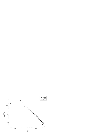
Figure 1: Average density of people $<\rho_{ij}>$ commuting from ward $i$ to ward $j$ as a function of the generalised time $t^{*}$ to travel from ward $i$ to ward $j$. The power law behaviour is a signature of the strong geographical dependence of the network.

We then define the degree density $\tau_{i}^{out/in}$ for ward $i$ as $\tau_{i}^{out/in}=\frac{k_{i}^{out/in}}{A_{i}}$ and the strength density $\sigma_{i}^{out/in}$ for ward $i$ as $\sigma_{i}^{out/in}=\frac{s_{i}^{out/in}}{A_{i}}$.

In section II we will show the main results of the empirical analysis of the data. In section III we will propose a simple model to reproduce the behaviour of commuters in the city.

II Empirical analysis

The network is composed by 634 vertices connected by 143102 edges with an average degree $<k>=226$, so that we can say it is a very well connected network indeed.

The out-degree density or out-connectivity density $\tau_{i}^{out}$ of the vertex $i$ is the number of different wards people living in the ward $i$ work in, divided for the area of the ward $i$, that is the area density of working connections a ward can create with other wards in London. It can be seen as a measure of the average commuting chances of a ward. The out-degree density, in this network, spans from values of 4.9, for $Darwin$ ward, to 501, for $Aldersgate$ ward. The average out-degree density is 142.8. Examples of wards with out-degree density around the average are: $St.Pancras$ $and$ $Somers$ $Town$ ward, $The$ $Wrythe$ ward, etc.. In the top left of Fig.2 the map of the geographical distribution of the wards out-degree density is shown. It is interesting to notice how wards are organized in zones well defined within this measure. In particular the light coloured ring around the center in Fig.2 looks to be a good zone to commute to any other area of London.

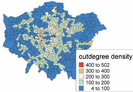
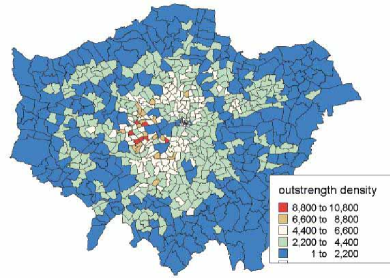
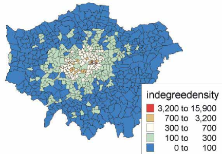
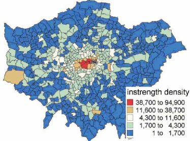
Figure 2: Maps of London showing the geographical distribution for: top left the out-degree density $\tau_{out}$; top right the out-strength density $\sigma_{out}$; bottom left the in-degree density $\tau_{in}$; bottom right the in-strength density $\sigma_{in}$.

The in-degree density or in-connectivity density $\tau_{i}^{in}$ of the vertex $i$ represents the number of wards people working in ward $i$ live in, divided for the area of ward $i$. It can be seen as a measure of the accessibility of a ward in respect of the other wards. The in-degree density, in this network, spans from values of 2, for $Darwin$ ward, to 15525, for $Walbrook$ ward. The average in-degree density is around 226. Examples of wards with in-degree density around the average are: $Canonbury$ ward, $Southfield$ ward, etc.. In the bottom left of Fig.2 it is shown the map of the geographical distribution of the wards’ in-degree density. From those maps it is possible to appreciate how this measure can identify the major business areas of London, where the in-degree is large, and the residential areas where the in-degree is small.

From these first results we can observe that the in-degree has a range of values that is larger by two orders of magnitude than that of the out-degree. This result reflects two very different phenomena behind the distribution process for settlement and business areas. This is due to the wards selectivity for urban function, where business tends to be concentrated in few areas while residential wards tend to spread over a much broader region.

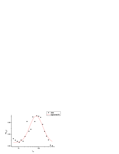
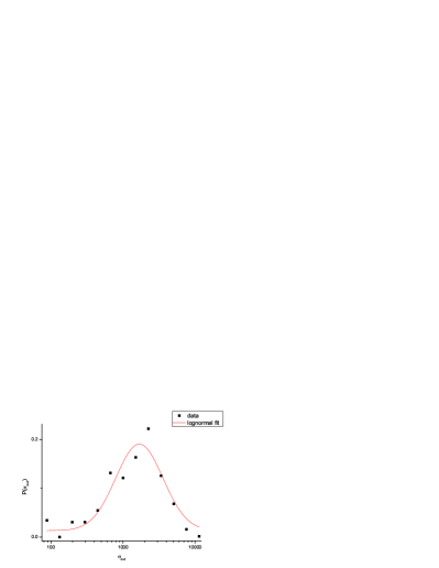
Figure 3: Top panels: Distribution for the out-degree density $\tau_{out}$. On the left the log-linear scale shows a log-normal shape, while the log-log scale on the right shows the power law behaviour in the tale of the distribution. Bottom panels:Distribution for the out-strength density $\sigma_{out}$. On the left the log-linear scale shows the log-normal shape, while the log-log scale on the right illustrates the power law behavior of the tale of the distribution.

The out-strength density $\sigma^{out}_{i}$ of the vertex $i$ represents the area density of employed people living in the ward $i$. The out-strength density values in our data span from a minimum of 70.20 for $Darwin$ ward, to a maximum of 10771.70 for $Earl^{\prime}s$ $Court$, with an average of 3051.38. Wards like $Golborne$, $Nunhead$, $Muswell$ $Hill$, etc are around the out-strength average values. The geographical distribution for the wards out-strength is given in the map in the upper right of Fig.2.

The in-strength density $\sigma^{in}_{i}$ of a vertex $i$ represents the total area density of people living in London who work in ward $i$, including ward $i$ itself. The in-strength density can be seen as a measure of the business capacity of a ward. The in-strength density values span from a minimum of 158.48 for $Darwin$ ward, to a maximum of 94805.70 for $St.James^{\prime}s$, with an average of 3027.27. Around the average in-strength density values we find wards like $Woodside$, $Hackney$ $Central$, $Cantelowes$, etc.. The geographical distribution for the wards in-strength is given in the map at the bottom right of Fig.2.

As we noticed before for the degree density, in this case we got that the out-strength density values range is just the $11\%$ of the in-strength density values range. In fact business areas tend to be concentrated in certain zones, defined by high values of in-strength. The out-strength values reflect the residential habits: the fact people tend to live in places that are more widely distributed around the whole city.

The differences between out and in vertex properties are better understood if we look at the experimental density distributions of probability for those quantities. In Fig.3 we show the out-degree/strength distributions. Since they’re very similar in shape, we can discuss them together. On the left we show the plots on a linear-log scale. In this way the shapes look very similar to log-normal distributions, that is the distribution of a measure whose logarithm is normally distributed. Nevertheless if we look at the same distributions on a log-linear scale we notice that the tail is a straight exponential.

In Fig.4 we show the in-degree and the in-strength distributions. As in the previous case the shapes are very similar. On a linear-log scale we find again the shape of a log-normal distribution. However the difference with the previous case is that when we look at the tail of the distribution on a log-log scale, we see that the distributions fall as a power law with exponent around $-2$.

In the next section we will give a simple interpretation of those results.

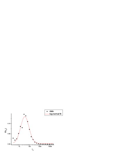
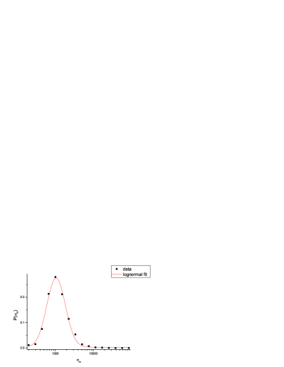
Figure 4: Top panels: Distribution for the in-degree density $\tau_{in}$. On the left the log-linear scale shows the log-normal shape, while the log-log scale on the right shows the power law behavior of the tale of the distribution. Bottom panels:Distribution for the in-strength density $\sigma_{in}$. On the left the log-linear scale shows the log-normal shape, while the log-log scale on the right shows the power law behavior of the tale of the distribution.

III The Model

To understand the statistical behaviour of the data, we focus on the fact that the phenomena we are dealing with, that is the metropolitan business centers and the metropolitan human residential settlements, are strictly related and influence each other during the growth of the city.

To understand the former phenomena, we have to look at the bottom right panel of Fig.2. The center of London, spreading from $the$ $City$ to $West$ $End$, has the biggest concentration of jobs in London, going away from this center the business centers gradually decrease. Then we can notice three other smaller business centers in the same map, $Heathrow$ in the west, $Croydon$ in the south and $Isle$ $of$ $Dogs$ east of the center. Analysing the nearest neighbour properties of those areas,we can see that, on a smaller scale, they reproduce the behaviour of central London.

The other strong evidence is that the strength and degree distributions have a peak and a power law tail with exponent around $-2$. This tail can be explained if we consider a distribution of points in a circle where the occupation probability $\Pi$ is proportional to the inverse of the square of the distance from the center $r$,

$$\Pi^{in}(r)\propto\frac{1}{r^{2}}.$$ (1)

If we define the in-strength $s^{in}$ in this case as the number of points falling in a certain area of the circle, then the in-strength will be completely dependent on the occupation process and we will have that $<s^{in}>\propto\frac{1}{r^{2}}$. To calculate the probability density function $P(s^{in})$ for the in-strength, we can calculate the probability density function for $r^{-2}$. In general we have that, if $<s^{in}>\propto r^{-\alpha}$, then $P(s^{in})=P(r^{-\alpha})\frac{dr^{-\alpha}}{ds^{in}}\propto P(r)r^{\alpha+1}\frac{dr^{-\alpha}}{ds^{in}}\propto s_{in}^{-1-2/\alpha}$. It is thus easy to see that, if $\alpha=2$, $P(s^{in})\propto s_{in}^{-2}$.

The peaked curve can be explained by the asymmetries of the city, that is London is not circular. To demonstrate this, we performed a simulation on a square lattice with 625 cells that we populated with 1875000 points with the probability given in Eq.1(these parameters are chosen to reproduce the London statistics). In the top left of Fig.5 we show the resulting map for the in strength while in the central panels of the same figure the resulting in-strength distribution. Those results have to be compared with the distribution in Fig4. Although we don’t capture the behaviour of the distribution for the values of the in-strength going to zero, we can notice that for the small values of the in-strength, the curves are very similar.

We can then assume that the in-strength distribution, that is the distribution of business metropolitan areas, is a geographical dependent variable. This means that once the business areas are settled, then they will grow just as an organism does, trying to be as compact as possible and with a radial homogeneous distribution.

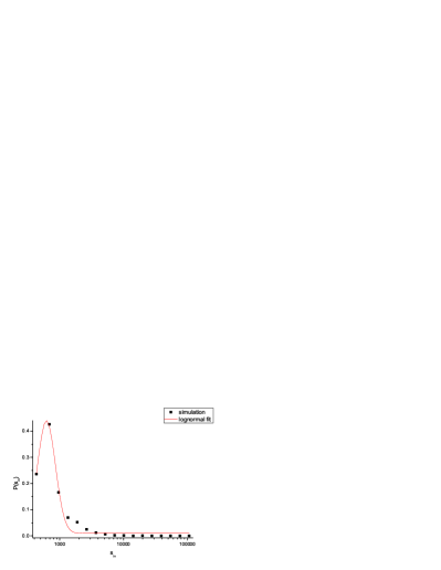
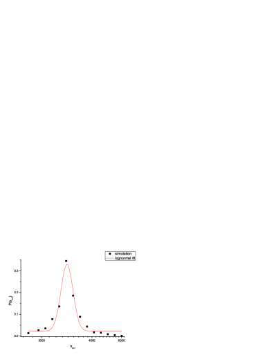
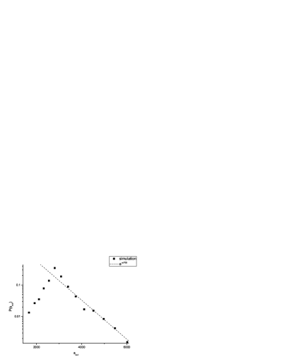
Figure 5: Square lattice simulation results. Top left panel: simulation for the in-strength, representing the business centers distribution. Top right: simulation for the out strength, representing the settlement distribution. Central panels: in-strength distribution: on the left the log-linear scale evidences the log-normal shape, while the log-log scale on the right evidences the power law behavior of the tale of the distribution. Bottom panels: distribution for the out-strength. On the left the log-linear scale evidences the log-normal shape, while the linear-log scale on the right evidences the exponential behavior of the tale of the distribution.

To understand the properties of the out-degree/strength distributions, that is where people decide to live, we can notice (Fig.2) that people tend to live close to their workplace, but not in the wards where there is a massive business activity. We interpret this observation in a stochastic growing model on the square lattice whose cells represent the wards of London. So, as we did for the in-strength distribution, we consider a square lattice with 625 cells. While the business centers are populated with the probability given in Eq.1, the residential ward $i$ will be populated with a probability given by:

$$\Pi^{out}_{i}\propto\frac{1}{s^{in}_{i}r_{i}^{2}},$$ (2)

where $r_{i}$ is the Euclidean distance from the ward $i$ to the center of the lattice. The probability in Eq.2 takes into account the fact that generally people tend to live close to their workplace with a rate that is proportional to the inverse of the square of $r$, but people don’t want to live in an area completely devoted to business, so with a inverse proportional dependence on the in-strength $s^{in}$ of the ward. The resulting simulated map for the out-strength is given in the top right panel of Fig.5. From the bottom panels of the same figure we can see that the probability distribution obtained for the out-strength possesses the required features, that is a peaked distribution with exponential tail.

IV Conclusions

In this work we analysed the network of commuters in London. Our empirical analysis is in itself important and unique. The data from 2001 census regarding the working habits of people of London are organised and contextualised in the framework of network theory. The organization of a city relies on many levels of complexity, from the social differences between people to the geographical constraints in the landscape of the city itself. Our research focuses on the organization seen as a result of phenomena related to the geographical locations of jobs and the accessibility of those places. We believe that in order to understand the organization of the city, those habits are the most important to consider, and actually London is the biggest and most productive city of western Europe.

We show that the power law for the distribution of business centers can be considered as the result of a pure geographical distribution of business areas, that is business centers tend to aggregate to preexisting business centers. In the model we propose the residential distribution in the city is described as a phenomena dependent on the distribution of business centers. This dependence on the business centers is shown to be $anti-preferential$, that is people want to be close to their place of work, but don’t want to live in an area devoted to business. The simulations seem to agree with the real data even if the model is minimal. In fact we showed how in London, beside the bigger activity center that is in Central London, other activity centers emerge at different scales. In our minimal model this effect is not considered, so that it can be seen as a model of local development that can be used at different scales.

- (1) A.L. Barabasi, R. Albert, H. Jeong, Physica A 272, 173 (1999).
- (2) M.Batty, Cities and Complexity, MIT Press (2007).
- (3) L. Euler, Comm. Acad. Sci. I. Petropol. 8, 128 (1736).
- (4) L. Euler, Novi Comm. Acad. Sci. Imp. Petropol. 4, 140 (1758).
- (5) Y. Hayashi, IPSJ Trans. Special Issue on Network Ecology 47, 776 (2006).
- (6) S.S. Manna, P. Sen, Phys. Rev. E 66, 066114 (2002).
- (7) A.F. Rozenfeld, R. Cohen, D. Ben-Avraham, S. Havlin, Phys. Rev. Lett. 89, 218701 (2002).
- (8) D. Volchenkov, P. Blanchard, Phys. Rev. E 75, 026104 (2007).
- (9) K. Yang, L. Huang, L. Yang, Phys. Rev. E 70, 015102(R) (2004).
- (10) http://www.statistics.gov.uk/census/
- (11) http://www.tfl.gov.uk/