LERW as an example of off-critical SLEs

Abstract

Two dimensional loop erased random walk (LERW) is a random curve, whose continuum limit is known to be a Schramm-Loewner evolution (SLE) with parameter $\kappa=2$. In this article we study “off-critical loop erased random walks”, loop erasures of random walks penalized by their number of steps. On one hand we are able to identify counterparts for some LERW observables in terms of symplectic fermions ($c=-2$), thus making further steps towards a field theoretic description of LERWs. On the other hand, we show that it is possible to understand the Loewner driving function of the continuum limit of off-critical LERWs, thus providing an example of application of SLE-like techniques to models near their critical point. Such a description is bound to be quite complicated because outside the critical point one has a finite correlation length and therefore no conformal invariance. However, the example here shows the question need not be intractable. We will present the results with emphasis on general features that can be expected to be true in other off-critical models.

Michel Bauer, Denis Bernard, Kalle Kytölä

1 Introduction

Over the last few years, our understanding of interfaces in two dimensional systems at criticality has improved tremendously. Schramm’s idea [26] to describe these interfaces via growth processes has met a great success. We are now in position to answer quantitatively in a routine way many questions of interest for physicists and/or mathematicians (the overlap is only partial, but non void).

All these successes suggest that we might try to be more ambitious and it seems that time has come to start thinking about what can be said for interfaces in non-critical systems. So far, the only attempts in this direction seem to be [8, 25], although also some yet unpublished work [24] will treat questions similar to this article in various models.

Needless to say, we do not aim to achieve general and definitive success in these notes. It is more our purpose to review some examples and see what we can say in each situation. We shall go a bit deeper into the specific example of loop erased random walks (LERW). This choice has a number of reasons. First, certain quantities for the LERW can be computed using only the underlying walk (with its loops kept), whose scaling limit is the familiar Brownian motion. This is the case for instance of boundary hitting probabilities. Second, the quantum field theory of the LERW is that of symplectic fermions, a free fermionic theory. This relationship is part of the standard lore at criticality, but it persists in the massive situation, and the specific perturbation we study is related to the Brownian local time, making it possible to compare closely the points of view of physics and mathematics.

To understand the difficulties inherent to the study of noncritical interfaces, it is perhaps worth spending some time on the physical and mathematical views concerning criticality and conformal invariance

In statistical mechanics on the lattice, for generic values of the parameters (collectively called $J$ here, examples include temperature, pressure, magnetic field, fugacity) the connected correlations among local observables decrease quickly (typically exponentially) with the distance : a correlation length $n(J)$ (in lattice units) can be defined and turns out to be of the order of a finite number of lattice mesh. Achieving a large $n(J)$ requires to adjust the parameters. Imagine we cover the plane (or approximate a fixed domain in the plane) with a lattice of mesh $a$, and tune the parameters $J$ in such a way that the macroscopic correlation length $an(J)=\zeta$ remains fixed while $a$ goes to $0$. Then it is expected on physical grounds that a limiting continuum theory exists, which may describe only some of the initial degrees of freedom in the system. Lattice translation symmetry becomes usual translation invariance in the limit. Rotation invariance is also very often restored. Over scales $s\gg a$ the discrete system is expected to be well approximated by the continuum theory.

In the limit $a\rightarrow 0$, $J$ tends to a limiting critical value $J_{c}$ (when several parameters are present this may be a critical manifold). The approach of $J$ to $J_{c}$ when $a\rightarrow 0$ is described by critical exponents. As $n(J_{c})$ is infinite, so is $an(J_{c})$ for any $a$, and the macroscopic correlation length is infinite at the critical point as well : the system has no characteristic length scale and the continuum limit is scale invariant. Over scales $s\ll\zeta$ the continuum off-critical system is expected to be well approximated by the critical system. On the lattice, an infinite number of control parameters can easily be exhibited, but if only their influence on the long distance physics is considered the equivalence classes form usually a finite dimensional space. Similarly, in the continuum limit, usually only a finite number of perturbations out of criticality are relevant.

For many two dimensional systems of interest, translation, rotation and scale invariance give local conformal invariance for free : the descriptions of the system in two conformally equivalent geometries are related by pure kinematics. This remarkable feature that emerges only in the continuum limit is suggested by convincing physical arguments but unproved in almost all cases of interest. The consequences of conformal invariance have been vigorously exploited by physicists for local observables since the 1984 and the seminal paper [7], even if the road to a complete classification of local two dimensional conformal field theories is still a distant horizon.

Schramm’s result in 1999 [26], on the other hand, is a complete classification of probability measures on random curves in (simply connected) domains of the complex plane (say joining two boundary points for definiteness) satisfying two axioms : conformal invariance and the domain Markov property. Again, the actual proof that a lattice interface has a limiting continuum description which satisfies the two axioms requires independent hard work. However the number of treated cases is growing rapidly, including the LERW, the Ising model, the harmonic navigator, percolation. A notorious exception which up to now has resisted to all attacks is the case of self avoiding walks.

Suppose that for each triple $({\mathbb{D}},x_{0},x_{\infty})$ consisting of a domain with two marked boundary points one has a probability measure on curves joining $x_{0}$ to $x_{\infty}$ (so we have the chordal case in mind). Consider an initial segment of curve, say $\gamma$, joining $x_{0}$ to a bulk point $x^{\prime}$ in ${\mathbb{D}}$. The domain Markov property relates the distribution of random curves in two situations : it states the equality of 1) the distribution of the rest of the random curve from $x^{\prime}$ to $x_{\infty}$ in ${\mathbb{D}}$ conditional on $\gamma$ and 2) the distribution of the random curve from $x^{\prime}$ to $x_{\infty}$ in ${\mathbb{D}}\backslash\gamma$.

This leads naturally to a description of the random curve as a growth process : if one knows how to grow an (infinitesimal) initial segment $\gamma$ in $({\mathbb{D}},x_{0},x_{\infty})$ from $x_{0}$ to $x_{\infty}$, one can apply the domain Markov property to build the rest of the curve as a curve in the cut domain $({\mathbb{D}}\backslash\gamma,x^{\prime},x_{\infty})$ and then conformal invariance to ”unzip” the cut i.e. map $({\mathbb{D}}\backslash\gamma,x^{\prime},x_{\infty})$ conformally to $({\mathbb{D}},x_{0},x_{\infty})$, so that another (infinitesimal) initial segment can be grown and mapped back to $({\mathbb{D}}\backslash\gamma,x^{\prime},x_{\infty})$ to get a larger piece of curve, and so on.

Technically, Schramm’s proof is made simpler by using the upper half plane $\mathbb{H}$ with $0$ and $\infty$ as marked points, with a time parameterization of the curve by (half) its capacity. Then the conformal map $g_{t}(z)$ that unzips the curve grown up to time $t$ and behaves at $\infty$ like $z+O(z^{-1})$ satisfies a Loewner differential equation $\frac{dg_{t}(z)}{dt}=\frac{2}{g_{t}(z)-\xi_{t}}$ which amounts to encoding the growing curve via the real continuous driving function $\xi_{t}$. It should be stressed that this representation is valid for any curve (or more generally any locally growing hull), independently of conformal invariance. However, the domain Markov property and conformal unzipping of the random curves straightforwardly translate into nice properties of the process $\xi_{t}$ : it has independent and stationary increments. Continuity yields that $\xi_{t}$ is a linear combination of a Brownian motion and time. Finally scale invariance, the conformal transformations fixing $({\mathbb{H}},0,\infty)$, leaves the sole possibility that $\xi_{t}=\sqrt{\kappa}B_{t}$ for some normalized Brownian motion $B_{t}$ and nonnegative scale factor $\kappa$.

Now suppose we consider the system out of criticality. Intuitively, there is no doubt that the probability that the interface has a certain topology with respect to a finite number of points in the domain should depend smoothly on the correlation length $\zeta$. But can we say a bit more ? Conformal invariance cannot be used to relate different domains and concentrating on the upper half plane case, as in the following, is really a choice. We can then describe the interface again by a Loewner equation for a $g^{\zeta}_{t}(z)$ with some (off-critical) source $\xi_{t}^{\zeta}$. What do we expect for this new random process?

At scales much smaller that the correlation length, i.e. in the ultraviolet regime, the deviation from criticality is small, and for instance the interface should look locally just like the critical interface. This means that over short time periods, the off-critical $\xi_{t}^{\zeta}$ should not be much different from its critical counterpart. Is is easily seen that if $\lambda>0$, the rescaled Loewner map $\frac{1}{\lambda}g_{\lambda^{2}t}(\lambda z)$ still satisfies the Loewner equation, but with a source $\frac{1}{\lambda}\xi_{\lambda^{2}t}^{\zeta}$. Taking a small $\lambda$ amounts to zoom at small scales near the origin and we expect that (in some yet unspecified topology) $\lim_{\lambda\rightarrow 0^{+}}\frac{1}{\lambda}\xi_{\lambda^{2}t}^{\zeta}$ exists and is a $\sqrt{\kappa}B_{t}$ for some normalized Brownian motion. As the interface looks like a critical interface not only close to the origin but close to any of its points, we also expect that $g_{s}^{\zeta}$ maps the interface to a curve that looks like a critical curve close to the origin, so that more generally for fixed $s$ the limit $\lim_{\lambda\rightarrow 0^{+}}\frac{1}{\lambda}(\xi_{s+\lambda^{2}t}^{\zeta}-\xi_{s}^{\zeta})$ should exist and be a $\sqrt{\kappa}B_{t}$. Hence to each fixed $s$ we can in principle define a Brownian motion. The Brownian motions defined for distinct $s$’s are moreover expected to be independent. To go further, we would need to have some control on how uniform in $s$ the convergence is, and how fast the correlations between $\frac{1}{\lambda}(\xi_{s+\lambda^{2}t}^{\zeta}-\xi_{s}^{\zeta})$ for distinct values of $s$ decrease with $\lambda$. There could be some problem with inversions of limits. In the nice situation, we would naively deduce for the above facts that the quadratic variation of $\xi_{t}^{\zeta}$ is exactly $\kappa t$ even at finite $\zeta$. This raises the question whether $\xi_{t}^{\zeta}$ can be represented as the sum of a Brownian motion (scaled by $\sqrt{\kappa}$) plus some process, contributing $0$ to the quadratic variation, but whose precise regularity would remain to be understood. Finally, the strongest relationship one could imagine between $\xi_{t}^{\zeta}$ and its critical counterpart $\xi_{t}$ would be that their laws are mutually absolutely continuous over finite time intervals. We shall see examples of this situation in the sequel, but at least one counterexample is known, off-critical percolation [25]. On the lattice, the set of interfaces is discrete, and the question of absolute continuity trivializes. One can write down discrete martingales describing the relative weight of an initial interface segment off/at criticality and a naive extrapolation to the continuum limit yields a candidate for the Radon-Nikodym derivative for the growth of the interface. This is the basis of much of the forthcoming discussion.

At scales large with respect to $\zeta$ however, i.e. in the infrared regime, the behavior is different and the interface should look like another SLE with a new $\kappa_{ir}$. Think of the Ising model for example. At criticality $\kappa=3$ but if the temperature is raised above the critical point, renormalization group arguments indicate that at large scale the interface looks like the interface at infinite temperature, i.e; percolation and $\kappa_{ir}=6$. One expects in general that $\lim_{\lambda\rightarrow+\infty}\frac{1}{\lambda}\xi_{\lambda^{2}t}^{\zeta}$ exists and is a $\sqrt{\kappa_{ir}}B_{t}$. This means that the process $\xi_{t}^{\zeta}$ could yield information on the flow of the renormalization group. Whether this can be used as an effective tool is unclear at the moment.

Let us close this introduction with the following observations. Conformal invariance and the domain Markov property have a rather different status. Whereas conformal invariance emerges (at best) in the continuum limit at criticality, the domain Markov property makes sense and is satisfied on the lattice without tuning parameters for many systems of interest. It can be considered as a manifestation of locality (in the physicists terminology). Hence the domain Markov property is still expected to hold off criticality. However the consequences of this property on $\xi_{t}^{\zeta}$ do not seem to have a simple formulation. As for conformal invariance, there is a trick to preserve it formally out of the critical point : instead of perturbing with a scaling field $O(z,\bar{z})$ times a coupling constant $\lambda$, perturb by a scaling field times a density $\lambda(z,\bar{z})$ of appropriate weight, in such a way that $\lambda(z,\bar{z})O(z,\bar{z})d\bar{z}\wedge dz$ is a $2$-form. This also gets rid of infrared divergences that occur in unbounded domain if $\lambda(z,\bar{z})$ has compact support. We shall use this trick in some places, but beware that if perturbation theory contains divergences, problems with scale invariance will arise, hence the cautious word ”formally” used above.

The paper is organized as follows. We start with a few examples in section 2. A brief account of SLEs, as appropriate for our needs, is given in section 3. Section 4 is devoted to the general philosophy of how one might hope to attack the question of interfaces in off-critical models. In particular we propose a field theoretical formula for Radon-Nikodym derivative between the off-critical and critical measures on curves. The main example of LERW is treated in detail in section 5. We discuss the critical and off-critical field theory for LERW, compute multipoint functions of the perturbing operator and subinterval hitting probabilities — and derive in two ways the off-critical driving process to first order in the magnitude of the perturbation.

2 Examples

To give some concreteness to the thoughts presented in the introduction, we will start with a couple of examples.

2.1 Self avoiding walks

Our first example deals with self avoiding walks (SAW). Consider a lattice of mesh size $a$ embedded in a domain $\mathbb{D}$ in the complex plane. A sample of a SAW is a simple nearest neighbor path on the lattice never visiting twice any lattice site. The statistics of SAW is specified by giving the weight $w_{\gamma}=x^{|\gamma|}$, with $|\gamma|$ the number of steps of $\gamma$ and $x$ the fugacity, to each path $\gamma$. The partition function $Z_{\mathbb{D}}$ is the sum $Z_{\mathbb{D}}=\sum_{\gamma}x^{|\gamma|}$ and the probability of occurrence of a curve $\gamma$ is $w_{\gamma}/Z_{\mathbb{D}}$.

There is a critical value $x_{c}$, depending on the lattice, for which typical sample consists of paths of macroscopic sizes so that the continuum limit $a\to 0$ can be taken. This continuum limit is conjectured to be conformally invariant and described by chordal SLE_8/3 if we restrict ourselves to SAW starting and ending at prescribed points on the boundary of $\mathbb{D}$.

The off-critical SAW model in the scaling regime consists of looking at SAW for fugacity $x$ close to its critical value $x_{c}$ (and approaching $x_{c}$ in a appropriate way as the mesh size goes to zero). The continuous limiting theory is not anymore conformally invariant as a scale parameter is introduced when specifying the way $x$ approaches its critical value. Renormalization group arguments tell us that if $x<x_{c}$ the fugacity flows to zero at large distances so that the partition function is dominated by the shortest path while if $x>x_{c}$ it flows to the critical value corresponding to uniform spanning trees (UST) so that the partition function is dominated by these space filling paths.

The off-critical partition function $\sum_{\gamma}x_{c}^{|\gamma|}(x/x_{c})^{|\gamma|}$ can be written as an expectation value with respect to the critical measure

$$Z_{\mathbb{D}}/Z^{c}_{\mathbb{D}}=\mathsf{E}[\,(x/x_{c})^{|\gamma|}\,]$$

with $Z^{c}_{\mathbb{D}}$ the critical partition function and $\mathsf{E}$ the critical measure. If a sample path $\gamma$ has a typical length scale $l_{\mathbb{D}}(\gamma)$, which is macroscopic in the critical theory, its number of steps scales as $|\gamma|\simeq(l_{\mathbb{D}}(\gamma)/a)^{d_{\kappa}}$ with $a$ the lattice mesh size and $d_{\kappa}$ the fractal dimension (more or less by definition of the fractal dimension). The scaling limit defining the continuous off-critical theory then consists of taking the limit $x\to x_{c}$ such that $\nu:=-a^{-d_{\kappa}}\log(x/x_{c})$ is finite as $a\to 0$, that is $(x-x_{c})/x_{c}\simeq-\nu\,a^{d_{\kappa}}$ as $a\to 0$. The parameter $\nu$ has scaling dimension $d_{\kappa}$ and introduces a scale and a typical correlation length $\zeta\simeq\nu^{-1/d_{\kappa}}$. This ensures that the relative weights $(x/x_{c})^{|\gamma|}\simeq e^{-\nu|\gamma|a^{d_{\kappa}}}$ have a finite limit for typical paths as the mesh size goes to zero. In the continuum the weights (relative the critical weights) are $e^{-\nu{L}_{\mathbb{D}}(\gamma)}$ with ${L}_{\mathbb{D}}(\gamma)\simeq l_{\mathbb{D}}(\gamma)^{d_{\kappa}}$ and the ratio of the off-critical partition function to the critical one is

$$\mathcal{Z}_{\mathbb{D}}=\mathsf{E}[\,e^{-\nu{L}_{\mathbb{D}}(\gamma)}\,].$$

In the continuum limit the critical curve should be described by SLEs and we’d like to understand what the above teaches us about the off-critical curves. Recall that SLE comes as a one parameter family SLE_κ, $\kappa>0$, and that critical SAW is conjectured to be described by SLE_8/3. For simplicity we consider here chordal SLE in which one looks for curves starting and ending at fixed points $x_{0},\ x_{\infty}$ on the boundary $\partial\mathbb{D}$ of $\mathbb{D}$. Recall that in the SLE construction the curves are given a ’time’ parametrization $\gamma:[0,T]\rightarrow\overline{\mathbb{D}}$, with $\gamma_{0}=x_{0}$, $\gamma_{T}=x_{\infty}$, such that the filtration associated to the knowledge of the curve up to time $t$, $(\mathcal{F}^{\gamma}_{t})_{t\in[0,T]}$, is the filtration generated by the Loewner driving process $(\xi_{t})_{t\in[0,T]}$, i.e. $\mathcal{F}^{\gamma}_{t}=\sigma\{\xi_{s}:0\leq s\leq t\}$ (for a reader not yet familiar with SLE, see section 3). The expectation $\mathsf{E}[\cdots]$ in the previous formula becomes the SLE measure. The mathematical definition of ${L}_{\mathbb{D}}(\cdot)$ is related to what is known as natural parametrization of the SLE curve [18, 21, 14]. It should satisfy the additivity property

$${L}_{\mathbb{D}}(\gamma_{[0,t+s]})={L}_{\mathbb{D}}(\gamma_{[0,t]})+{L}_{\mathbb{D}\setminus\gamma_{[0,t]}}(\gamma_{[t,t+s]}),$$

or even the stronger property that the natural parameterization of a piece of SLE can be defined without reference to the domain, and ${L}(\gamma_{[0,t+s]})={L}(\gamma_{[0,t]})+{L}(\gamma_{[t,t+s]}),$ since ${L}(\gamma)$ is naively proportional to the number of steps of $\gamma$. We shall later define in a more general context the notion of an interface energy and see that it possesses an analogous additivity property.

The factor $e^{-\nu{L}_{\mathbb{D}}(\cdot)}$ specifies the Radon-Nikodym derivative of the off-critical measure with respect to the critical SLE measure so that the off-critical expectation of an observable ${\cal O}$ is

$$\mathsf{E}^{\nu}[\,{\cal O}\,]=\mathcal{Z}_{\mathbb{D}}^{-1}\,\mathsf{E}[\,e^{-\nu{L}_{\mathbb{D}}(\cdot)}\,{\cal O}\,]\quad{\rm with}\quad\mathcal{Z}_{\mathbb{D}}=\mathsf{E}[\,e^{-\nu{L}_{\mathbb{D}}(\cdot)}\,].$$

If ${\cal O}$ is $\mathcal{F}^{\gamma}_{t}$-measurable, that is if ${\cal O}$ only depends on the knowledge of the curve up to time $t$, we have

$$\mathsf{E}^{\nu}[\,{\cal O}\,]=\mathsf{E}[\,M_{t}\,{\cal O}\,]\quad{\rm with}\quad M_{t}:=\mathcal{Z}_{\mathbb{D}}^{-1}\,\mathsf{E}[e^{-\nu{L}_{\mathbb{D}}(\cdot)}|\mathcal{F}^{\gamma}_{t}]$$

since $\mathsf{E}[\,e^{-\nu{L}_{\mathbb{D}}(\cdot)}\,{\cal O}]=\mathsf{E}[\,\mathsf{E}[\,e^{-\nu{L}_{\mathbb{D}}(\cdot)}\,{\cal O}|\mathcal{F}^{\gamma}_{t}\,]\,]=\mathsf{E}[\,M_{t}\,{\cal O}\,]$ because we can take out what is known, $\mathsf{E}[\,e^{-\nu{L}_{\mathbb{D}}(\cdot)}\,{\cal O}|\mathcal{F}^{\gamma}_{t}\,]={\cal O}\,\mathsf{E}[\,e^{-\nu{L}_{\mathbb{D}}(\cdot)}|\mathcal{F}^{\gamma}_{t}\,]$.

In other words, the off-critical SLE (corresponding to the perturbation by the natural parametrization) is obtained by weighting the SLE expectation with $M_{t}$. As a conditional expected value, $M_{t}$ is by construction a martingale and $M_{0}=1$ so that $\mathsf{E}^{\nu}$ is correctly normalized to be a probability measure. Notice that, modulo a few regularity assumptions, this is the framework in which Girsanov’s theorem applies, as will be discussed in section 4.3. The additivity property of the natural parametrization implies that $M_{t}=e^{-\nu{L}_{\mathbb{D}}(\gamma_{[0,t]})}\,\mathcal{Z}_{\mathbb{D}}^{-1}\,\mathsf{E}[e^{-\nu{L}_{\mathbb{D}\setminus\gamma_{[0,t]}}(\cdot)}]$ so that

$$M_{t}=e^{-\nu{L}_{\mathbb{D}}(\gamma_{[0,t]})}\,\frac{\mathcal{Z}_{\mathbb{D}\setminus\gamma_{[0,t]}}}{\mathcal{Z}_{\mathbb{D}}}\textrm{ .}$$ (1)

$M_{t}$ can naturally be interpreted as the off-critical weight (relative to the critical one) given to the curve $\gamma_{[0,t]}$. It is made of two contributions, one is a ratio of partition functions in the cut domain $\mathbb{D}\setminus\gamma_{[0,t]}$ and in $\mathbb{D}$, the other is an ’interface energy’ contribution $\nu{L}_{\mathbb{D}}(\gamma_{[0,t]})$ associated to the curve. We shall recover this decomposition in a more general (but more formal) context of perturbed SLEs in following sections.

2.2 Loop erased random walks

The second example deals with loop erased random walks (LERW) and it will be further developed in section 5. Let us first recall the definition of a LERW. Again let us start with a lattice $\mathbb{D}^{(a)}$ of mesh $a$ embedded in a domain $\mathbb{D}$. Given a path $W=(W_{0},W_{1},\cdots,W_{n})$ on the lattice its loop erasure $\gamma$ is defined as follows: let $n_{0}=\max\{m:W_{m}=W_{0}\}$ and set $\gamma_{0}=W_{n_{0}}=W_{0}$, next let $n_{1}=\max\{m:W_{m}=W_{n_{0}+1}\}$ and set $\gamma_{1}=W_{n_{1}}$, and then inductively let $n_{j+1}=\max\{m:W_{m}=W_{n_{j}+1}\}$ and set $\gamma_{j}=W_{n_{j}}$. This produces a simple path $\gamma=\mathcal{L}(W)=(\gamma_{0},\gamma_{1},\ldots,\gamma_{l})$ from $\gamma_{0}=W_{0}$ to $\gamma_{l}=W_{n}$, called the loop-erasure of $W$, but its number of steps $l$ is in general much smaller than that of the original path $W$. We emphasize that the starting and end points are not changed by the loop-erasing.

We point out that the above definition of loop erasure is equivalent to the result of a recursive procedure of chronological loop erasing: the loop erasure of a $0$ step path $(W_{0})$ is itself, $\gamma=(W_{0})$ and if the erasure of $W=(W_{0},\ldots,W_{m})$ is the simple path $\mathcal{L}(W)=(\gamma_{0},\ldots,\gamma_{l})$ then for the loop erasure of $W^{\prime}=(W_{0},\ldots,W_{m},W_{m+1})$ there are two cases depending on whether a loop is formed on step $m+1$. If $W_{m+1}\notin\{\gamma_{0},\ldots,\gamma_{l}\}$ then the loop erasure of $W^{\prime}$ is $\gamma^{\prime}=(\gamma_{0},\ldots,\gamma_{l},W_{m+1})$. But if a loop is formed, $W_{m+1}=\gamma_{k}$ for some $k\leq l$ (unique because $\gamma$ is simple), then the loop erasure of $W^{\prime}$ is $\gamma^{\prime}=(\gamma_{0},\ldots,\gamma_{k})$.

In this paper we shall be interested in paths starting at a boundary point ${x_{0}}$ and ending on a subset $S$ of the boundary of $\mathbb{D}$.

Statistics of LERW is defined by associating to any simple path $\gamma$ a weight $w_{\gamma}=\sum_{W:\mathcal{L}(W)=\gamma}\mu^{|W|}$, where the sum is over all nearest neighbor paths $W$ whose erasures produce $\gamma$, and $|W|$ denotes the number of steps of $W$. There is a critical value $\mu_{c}$ of the fugacity at which the underlying paths $W$ become just ordinary random walks. The partition function $\sum_{\gamma}w_{\gamma}$ of LERWs from $z$ to $S$ in $\mathbb{D}$ can be rewritten as a sum over walks in the domain $\mathbb{D}$, started from $z$ and counting only those that exit the domain through set $S$

$$Z^{\mathbb{D};z;S}_{\mathrm{RW}}\;=\;\sum_{\begin{subarray}{c}\gamma\textrm{ simple path}\\ \textrm{from $z$ to $S$ in $\mathbb{D}$}\end{subarray}}w_{\gamma}\;=\;\sum_{\begin{subarray}{c}W\textrm{ walk from}\\ \textrm{$z$ to $S$ in $\mathbb{D}$}\end{subarray}}\mu^{|W|}\textrm{ .}$$

Written in terms of critical random walks, the partition function thus reads $\mathsf{E}^{z}_{\mathrm{RW}}\big{[}(\mu/\mu_{c})^{|W|}\;\mathbf{1}_{W_{\tau^{\mathrm{RW}}_{\mathbb{D}}}\in S}\big{]}$, where $\tau^{\mathrm{RW}}_{\mathbb{D}}$ denotes the exit time of the random walk $W$ from $\mathbb{D}$.

Critical LERW corresponds to the critical fugacity and is described by SLE₂, see [26, 19, 31]. For $\mu<\mu_{c}$ — which is the case we shall consider — paths of small lengths are more favourable and renormalization group arguments tell that at large distances the path of smallest length dominates. The off-critical theory in the scaling regime corresponds to non critical fugacity $\mu$ but approaching the critical one as the mesh size tends to zero. At fixed typical macroscopic size, the number of steps of typical critical random walks (not of their loop erasures) scales as $a^{-2}$, so that the scaling limit is such that $\nu:=-a^{-2}\log(\mu/\mu_{c})$ is finite as $a\to 0$, ie. $(\mu-\mu_{c})/\mu_{c}\simeq-\nu\,a^{2}$ and $\nu$ has scaling dimension $2$ and fixes a mass scale $m\simeq\sqrt{\nu}$ and a correlation length $\zeta\simeq 1/m$. In this scaling limit the weights become $(\mu/\mu_{c})^{|W|}\simeq e^{-\nu a^{2}|W|}$ and the random walks converge to two dimensional Brownian motions $\bf{B}$ with $a^{2}|W|=a^{2}\tau^{\mathrm{RW}}_{\mathbb{D}}$ converging to the times $\tau_{\mathbb{D}}$ spent in $\mathbb{D}$ by $\bf{B}$ before exiting. The off-critical partition function can thus be written as a Brownian expectation value $Z^{\mathbb{D};z;S}_{\nu}\longrightarrow\mathsf{E}^{z}_{\mathrm{BM}}\big{[}\,e^{-\nu\tau_{\mathbb{D}}}\,\mathbf{1}_{\bf{B}_{\tau_{\mathbb{D}}}\in S}\,\big{]}$ as $a\downarrow 0$. We may generalize this by letting $\nu$ vary in space: steps out of site $w\in\mathbb{D}$ are given weight factor $\mu(w)=\mu_{c}\;e^{-a^{2}\nu(w)}$ , in which case the partition function is

$$Z^{\mathbb{D};z;S}_{\nu}=\mathsf{E}^{z}_{\mathrm{RW}}\big{[}\,e^{-\sum_{0\leq j<\tau^{\mathrm{RW}}_{\mathbb{D}}}a^{2}\nu(W_{j})}\,\mathbf{1}_{W_{\tau^{\mathrm{RW}}_{\mathbb{D}}}\in S}\,\big{]}\underset{a\downarrow 0}{\longrightarrow}\mathsf{E}^{z}_{\mathrm{BM}}\big{[}\,e^{-\int_{0}^{\tau_{\mathbb{D}}}\nu({\bf{B}}_{s})\,\mathrm{d}s}\,\mathbf{1}_{{\bf{B}}_{\tau_{\mathbb{D}}}\in S}\,\big{]}\textrm{ .}$$

The explicit weighting by $e^{-\nu\tau^{\mathrm{RW}}_{\mathbb{D}}}$ is transparent for the random walk, but becomes less concrete for the LERW since the same path $\gamma$ can be produced by random walks of different lengths and by walks that visit different points. Compared to the previous example of SAW, the description of the off-critical LERW theory via SLE martingales is thus more involved but will (partially) be described in following sections.

2.3 Percolation

We will briefly also mention the case of off-critical percolation, just for some comparisons. A way to study the scaling limit in the off-critical regime was suggested in [8].

It is most convenient to define interfaces in percolation on the hexagonal lattice. A configuration $\omega$ of face percolation on lattice domain $\mathbb{D}$ with lattice spacing $a$ is a colouring of all faces (hexagons) to open (1) or closed (0), i.e. $\omega\in\{0,1\}^{F_{\mathbb{D}}}$, where $F_{\mathbb{D}}$ is the set of faces. The Boltzmann weight of a configuration is $w_{\omega}=p^{\#\mathrm{open}(\omega)}(1-p)^{\#\mathrm{closed}(\omega)}$ — that is hexagons are chosen open with probability $p$ independently. This hexagonal lattice face percolation (triangular lattice site percolation) is critical at $p=p_{c}=1/2$ and has been proven to be conformally invariant [28]. Exploration path, an interface between closed and open clusters, is described in the continuum limit by SLE₆. Note also that

$$Z_{\mathbb{D}}=\sum_{\omega}p^{\#\mathrm{open}(\omega)}(1-p)^{\#\mathrm{closed}(\omega)}=\prod_{z\in F_{\mathbb{D}}}(p+(1-p))=1$$

for any $p\in(0,1)$.

The off-critical regime now consists of changing the state of some faces that are macroscopically pivotal, i.e. affect connectivity properties to macroscopic distances. Informally, these faces are such that from their neighborhood there exists four paths of alternating colors to a macroscopic distance away from the point. The number of such points in the domain $\mathbb{D}$ should be of order $|\mathbb{D}|\times a^{-3/4}$, so that in order to have finite probability of changing a macroscopically pivotal face we should take $|p-p_{c}|\sim a^{3/4}$. We denote the perturbation amplitude by $\nu=a^{-3/4}\log(\frac{p}{p_{c}})$.

For more about interfaces in off-critical percolation, the reader should turn to [8, 25]. The above remarks will be enough for us to give a point of comparison.

3 SLE basics

The method of Schramm-Loewner evolutions (SLE) is a significant recent development in the understanding of conformally invariant interfaces in two dimensions. We will describe the main ideas briefly and informally, and refer the reader to the many reviews of the topic, e.g. [17, 29, 12, 1, 11], among which one can choose according to the desired level of mathematical rigour, physical intuition, emphasis and prerequisite knowledge.

3.1 Chordal SLE in the standard normalization

It was essentially shown in [26] that with assumptions of conformal invariance and domain Markov property, probability measures on random curves in a simply connected domain $\mathbb{D}$ from a point $x_{0}\in\partial\mathbb{D}$ to $x_{\infty}\in\partial\mathbb{D}$ are classified by one parameter, $\kappa\geq 0$. These random curves are called chordal SLE_κ.

The curves SLE_κ are simple curves (no double points) iff $0\leq\kappa\leq 4$. For the purposes of this paper simple curves are enough, so we restrict ourselves to this least complicated case. To describe the chordal SLE_κ, we note that by the assumed conformal invariance it suffices to discuss it in the domain $\mathbb{H}=\{z\in\mathbb{C}:\Im\textrm{m }z>0\}$ (upper half plane) from $0$ to $\infty$ — for any other choice of $\mathbb{D},{x_{0}},{x_{\infty}}$ one applies a conformal map $f:\mathbb{H}\rightarrow\mathbb{D}$ such that $f(0)=x_{0}$, $f(\infty)=x_{\infty}$. The existence of such $f$ follows from Riemann mapping theorem and well-definedness of the resulting curve ($f$ is only unique up to composition with a scaling $z\mapsto\lambda z$ of $\mathbb{H}$) from the scale invariance of chordal SLE.

So, let $0\leq\kappa\leq 4$ and let $g_{t}(z)$ be the solution of the Loewner’s equation

$$\frac{\mathrm{d}}{\mathrm{d}t}g_{t}(z)=\frac{2}{g_{t}(z)-\xi_{t}}$$ (2)

with initial condition $g_{0}(z)=z\in\mathbb{H}$ and $\xi_{t}=\sqrt{\kappa}B_{t}$ a Brownian motion with variance parameter $\kappa$. The solution exists up to time $t$ for $z\in\mathbb{H}\setminus\gamma[0,t]$, where $\gamma:[0,\infty]\rightarrow\overline{\mathbb{H}}$ is a random simple curve such that $\gamma_{0}=0$ and $\gamma_{\infty}=\infty$. This curve is called the (trace of) chordal SLE_κ. Furthermore, $g_{t}$ is the unique conformal map from $\mathbb{H}\setminus\gamma[0,t]$ to $\mathbb{H}$ with the hydrodynamic normalization $g_{t}(z)=z+\mathcal{O}(z^{-1})$ as $z\rightarrow\infty$.

3.2 Chordal and dipolar SLEs in the half plane

The Loewner’s equation (2) can be used to describe any simple curve in $\mathbb{H}$ starting from the boundary $\partial\mathbb{H}=\mathbb{R}$ in the sense that $g_{t}$ is the hydrodynamically normalized conformal map from the complement of an initial segment of the curve to the half plane. In particular, a chordal SLE_κ in $\mathbb{H}$ from $x_{0}\in\mathbb{R}$ to $x_{\infty}\in\mathbb{R}$ is obtained by letting $\xi_{0}={x_{0}}$, $\eta_{0}={x_{\infty}}$ and $\xi_{t}$, $\eta_{t}$ solutions of the Itô differential equations

$$\begin{cases}\mathrm{d}\xi_{t}\;=\;\sqrt{\kappa}\;\mathrm{d}B_{t}+\frac{\rho_{c}}{\xi_{t}-\eta_{t}}\;\mathrm{d}t&\\ \mathrm{d}\eta_{t}\;=\;\frac{2}{\eta_{t}-\xi_{t}}\;\mathrm{d}t&\qquad\textrm{ that is }\eta_{t}=g_{t}(x_{\infty})\end{cases}$$

with $\rho_{c}=\kappa-6$, see e.g. [27, 6]. The maximal time interval of the solution is $t\in[0,T]$, where $T$ is a (random) stopping time and $\gamma_{T}=x_{\infty}$.

Another interesting case is a curve in $\mathbb{H}$ depending on the starting point $x_{0}$ and two other points $x_{+}<x_{-}$ such that $x_{0}\notin[x_{+},x_{-}]$. If the two points play a symmetric role, then the appropriate random conformally invariant curve is the dipolar SLE_κ [4]. We again have the Loewner’s equation (2) with $\xi_{0}={x_{0}}$, $X^{\pm}_{0}=x_{\pm}$ and Itô differential equations

$$\begin{cases}\mathrm{d}\xi_{t}\;=\;\sqrt{\kappa}\;\mathrm{d}B_{t}+\frac{\rho_{d}}{\xi_{t}-X^{+}_{t}}\;\mathrm{d}t+\frac{\rho_{d}}{\xi_{t}-X^{-}_{t}}\;\mathrm{d}t&\\ \mathrm{d}X^{\pm}_{t}\,=\,\frac{2}{X^{\pm}_{t}-\xi_{t}}\;\mathrm{d}t&\qquad\textrm{ that is }X^{\pm}_{t}=g_{t}(x_{\pm})\end{cases}$$

with $\rho_{d}=\frac{\kappa-6}{2}$. Again dipolar SLE is defined for $t\in[0,T]$, where $T>0$ is (random) stopping time such that $\gamma_{T}\in[x_{+},x_{-}]$.

Both these examples can be understood from the point of view of statistical physics in such a way that the (regularized) partition function for the model in $\mathbb{H}$ is $Z(x_{0},x_{\infty})=|x_{\infty}-x_{0}|^{\rho_{c}/\kappa}$ for the chordal SLE_κ and $Z(x_{0},x_{+},x_{-})=|x_{-}-x_{0}|^{\rho_{d}/\kappa}\;|x_{+}-x_{0}|^{\rho_{d}/\kappa}\;|x_{-}-x_{+}|^{\rho_{d}^{2}\,/\,2\kappa}$ for the dipolar SLE_κ. The driving process satisfies $\mathrm{d}\xi_{t}=\sqrt{\kappa}\;\mathrm{d}B_{t}+\kappa(\partial_{\xi}\log Z)\;\mathrm{d}t$ and other points follow the flow $g_{t}$. For discussion of more general SLE variants of this kind see [6, 15, 16, 1].

4 Probability measures

4.1 Definition from discrete stat. mech. models

Let us first recall how measures on curves are defined in statistical physics models via Boltzmann weights. We have in mind Ising like models. Let $\mathcal{C}$ be the configuration space of a lattice statistical model defined on a domain $\mathbb{D}$. For simplicity we assume $\mathcal{C}$ to be discrete and finite but as large as desired. Let $w_{c}$, $w_{c}\geq 0$, $c\in{\cal C}$, be the Boltzmann weights and $Z_{\mathbb{D}}$ the partition function, $Z_{\mathbb{D}}:=\sum_{c\in\mathcal{C}}\ w_{c}$. By Boltzmann rules, the probability of a configuration $c$ is $\mathsf{P}[\{c\}]:=w_{c}/Z_{\mathbb{D}}$, and this makes $\mathcal{C}$ a probability space.

In the present context, imagine that specific boundary conditions are imposed in such a way as to ensure the presence of an interface in $\mathbb{D}$ for any sample – for simplicity we consider only one interface. Given a curve $\gamma$ in $\mathbb{D}$, that we aim at identifying as an interface, there exists a subset of configurations $\mathcal{C}_{\gamma}$ for which the actual interface coincides with the prescribed curve $\gamma$. Again by Boltzmann rules, the probability of occurrence of the curve $\gamma$ as an interface, i.e. the probability of the event $\mathcal{C}_{\gamma}$, is the ratio of the partition functions

$$\mathsf{P}_{\mathbb{D}}[\mathcal{C}_{\gamma}]=Z_{\mathbb{D}}[\gamma]/Z_{\mathbb{D}}.$$ (3)

where $Z_{\mathbb{D}}[\gamma]$ is the conditioned partition function defined by the restricted sum

$$Z_{\mathbb{D}}[\gamma]:=\sum_{c\in\mathcal{C}_{\gamma}}w_{c}~{}.$$

The Boltzmann weights may depend on parameters such that for critical values the statistical model is critical. We denote by $\mathsf{P}_{\mathbb{D}}^{0}$ the probability measure at criticality, with Boltzmann weight $w^{0}$, which in the continuum is expected to become an SLE measure if only the statistics of the interface are considered. We generically denote by $\mathsf{P}_{\mathbb{D}}^{\nu}$ the off-critical measures, with Boltzmann weights $w^{\nu}$. These probability measures differ by a density:

$$\mathsf{P}_{\mathbb{D}}^{\nu}=M^{\nu}_{\mathbb{D}}\ \mathsf{P}_{\mathbb{D}}^{0}$$

where, by construction, $M^{\nu}_{\mathbb{D}}$ are defined as ratio of partition functions (again, no degrees of freedom other than the shape of the interface are considered):

$$M^{\nu}_{\mathbb{D}}=\frac{Z^{\nu}_{\mathbb{D}}[\gamma]/Z^{0}_{\mathbb{D}}[\gamma]}{Z^{\nu}_{\mathbb{D}}/Z^{0}_{\mathbb{D}}}\ .$$

As in our previous examples, $M^{\nu}_{\mathbb{D}}$ code for the off-critical weights relative to the critical ones. On a finite lattice, they are typically well defined but their existence in the continuum limit may be questioned. This has to be analysed case by case.

Assume as in the SLE context that the interfaces emerge from the boundary of $\mathbb{D}$ so that the cut domains $\mathbb{D}\setminus\gamma$ are also domains of the complex plane. The restricted partition function $Z_{\mathbb{D}}[\gamma]$ is then proportional to the partition function in the cut domain

$$Z_{\mathbb{D}}^{\nu}[\gamma]=e^{{\cal E}^{\nu}_{\mathbb{D}}(\gamma)}Z^{\nu}_{\mathbb{D}\setminus\gamma}\textrm{ .}$$

The extra term ${\cal E}^{\nu}_{\mathbb{D}}(\gamma)$ arises from the energy of the lattice bonds which have been cut from $\mathbb{D}$ to make $\mathbb{D}\setminus\gamma$. We call it the ’interface energy’ of $\gamma$. It inherits from the domain Markov property an additivity identity similar to the one satisfied by the natural parameterization, i.e.

$${\cal E}^{\nu}_{\mathbb{D}}(\gamma.\gamma^{\prime})={\cal E}^{\nu}_{\mathbb{D}}(\gamma)+{\cal E}^{\nu}_{\mathbb{D}\setminus\gamma}(\gamma^{\prime})\textrm{ .}$$

where $\gamma.\gamma^{\prime}$ is the concatenation of successive segments of the interface.

The off-critical weights then read:

$$M^{\nu}_{\mathbb{D}}(\gamma)=e^{{\cal E}_{\mathbb{D}}^{\nu}(\gamma)-{\cal E}_{\mathbb{D}}^{0}(\gamma)}\ \frac{Z^{\nu}_{\mathbb{D}\setminus\gamma}/Z^{0}_{\mathbb{D}\setminus\gamma}}{Z^{\nu}_{\mathbb{D}}/Z^{0}_{\mathbb{D}}}.$$ (4)

This can be compared with (1). The presence of the energy term ${\cal E}_{\mathbb{D}}^{\nu}(\gamma)-{\cal E}_{\mathbb{D}}^{0}(\gamma)$ in the continuum has also to be analysed case by case, see below. We furthermore point out that there may be several natural choices of what to include in the Boltzmann weights and different choices may lead to different ${\cal E}_{\mathbb{D}}^{\nu}$ term — to the extent that vanishing of this term can be a question of convention.

To make contact with SLE, we also define a stochastic growth process that describes the curve, in terms of which we define a filtration on $\mathcal{C}$. Consider portions of interfaces $\gamma[0,t]$, where the index $t$ specify say their lengths and will be identified with the ‘time’ of the process. We may partition our configuration space according to these portions at time $t$. The elements of the partition $\mathcal{Q}_{t}$ are denoted by $\mathcal{C}_{\gamma_{[0,t]}}$, indexed by $\gamma[0,t]$ in such a way that $c\in\mathcal{C}_{\gamma[0,t]}$ if and only if the configuration $c$ gives rise to $\gamma[0,t]$ as a portion of the interface. Thus we have $\mathcal{C}=\bigcup_{\gamma[0,t]}\mathcal{C}_{\gamma[0,t]}$, with $\mathcal{C}_{\gamma[0,t]}$ all disjoint. By convention $\mathcal{Q}_{0}$ is the trivial partition with the whole configuration space $\mathcal{C}$ as its single piece. We assume these partitions to be finer as $t$ increases because specifying longer and longer portions of interfaces defines finer and finer partitions. This means that for any $s>t$ and any element $\mathcal{C}_{\gamma[0,t]}$ of the partition at time $t$ there exist elements of $\mathcal{Q}_{s}$ which form a partition of $\mathcal{C}_{\gamma[0,t]}$ (corresponding to those $\gamma[0,s]$ which extend $\gamma[0,t]$). To any partition $\mathcal{Q}_{t}$ is associated a $\sigma$-algebra $\mathcal{F}^{\gamma}_{t}$ on $\mathcal{C}$, the one generated by the elements of this partition. Since these partitions are finer as ‘time’ $t$ increases, these constitute a filtration $(\mathcal{F}^{\gamma}_{t})_{t\geq 0}$ on $\mathcal{C}$, i.e. $\mathcal{F}^{\gamma}_{t}\subset\mathcal{F}^{\gamma}_{s}$ for $s>t$. The fact that we trivially get a filtration simply means that increasing ‘time’ $t$ increases the knowledge on the system. In the SLE context the information about the curve is encoded in the driving process $(\xi_{t})_{t\geq 0}$, so this filtration $(\mathcal{F}^{\gamma}_{t})_{t\geq 0}$ becomes the one generated by $\xi$.

On ${\cal C}$ with the filtration $(\mathcal{F}^{\gamma}_{t})_{t\geq 0}$, we may define two processes using either the critical $\mathsf{P}^{0}$ or the off-critical $\mathsf{P}^{\nu}$ probability measures. They differ by $M^{\nu}_{\mathbb{D}}(\gamma[0,t])$ which can then be written as a conditioned expectation with respect to the critical measure

$$M^{\nu}_{\mathbb{D}}(\gamma[0,t])=\frac{Z_{\mathbb{D}}^{0}}{Z_{\mathbb{D}}^{\nu}}\ \mathsf{E}[\,\frac{w^{\nu}}{w^{0}}\,|\mathcal{F}^{\gamma}_{t}\,]$$

Thus $M_{\mathbb{D}}^{\nu}(\gamma[0,t])$ is a $P_{\mathbb{D}}^{0}$-martingale and the two processes differ by a martingale, which is the context in which Girsanov theorem applies. It is similar to what we encountered in the SAW example. One of our aims is to (try to) understand how this tautological construction applies in the continuum.

4.2 Continuum limit

4.2.1 Massive continuum limits in field theory

In the continuum limit, the critical model should be described by a conformal field theory (CFT) and the critical measure on curves by SLE. The Boltzmann weights are $e^{-S}$ with $S$ the action. Off-critical perturbation is generated by a so-called perturbing field $\Phi$ so that

$$S=S^{0}+\nu\int_{\mathbb{D}}d^{2}z\,\Phi(z,\bar{z})$$

with $S^{0}$ the conformal field theory action. The ratio of the (off-critical) field theory partition function to the CFT (critical) one is the expectation value

$$\frac{\langle\exp[-\nu\int_{\mathbb{D}}d^{2}z\,\Phi(z,\bar{z})]\;(\mathrm{bdry}\;\mathrm{cond.})\rangle_{\mathbb{D}}}{\langle(\mathrm{bdry}\;\mathrm{cond.})\rangle_{\mathbb{D}}}$$ (5)

where the brackets denote CFT expectations and the boundary conditions $(\mathrm{bdry}\;\mathrm{cond.})$ are implemented by insertion of appropriate boundary operators, including in particular the operators that generate the interface.

The coupling constant $\nu$ has dimension $2-h-\overline{h}$, linked to the scaling dimension $h+\overline{h}$ of the perturbing operator $\Phi$. In our previous examples we determined explicitly this dimension by looking at the way the scaling limit is defined. We got (the perturbing operators in all cases are spinless, $h=\overline{h}$):
(i) SAW: $\nu$ has dimension $d_{\kappa}=1+\kappa/8$, i.e. $d_{8/3}=4/3$ for $\kappa=8/3$ which is the value corresponding to the SAW. The perturbing operator has dimension $h_{\kappa}+\overline{h}_{\kappa}=1-\kappa/8$, i.e. $h=\overline{h}=1/3$ for SAW. It is the operator $\Phi_{0;1}$ which is known to be the operator testing for the presence of the SLE curve in the neighbourhood of its point of insertion (in particular its one-point function gives the probability for the SLE curve to visit a tiny neighbourhood of a point in the complex plane, [3]). This had to be expected since the perturbation by the natural parametrization as described in the first section just counts the number of lattice size boxes crossed by the curve.
(ii) LERW: the coupling constant has dimension $2$ so that the perturbing operator has dimension $h=\overline{h}=0$ (up to logarithmic correction). We shall identify it either in terms of symplectic fermions or in terms of Brownian local time in the following sections.
(iii) Percolation: the coupling constant has dimension $3/4$ and therefore the perturbing operator should have $h=\overline{h}=5/8$. This operator is the bulk four-leg operator $\Phi_{0,2}$ testing for the presence of a macroscopically pivotal point.

4.2.2 Curves, RN-derivatives and interface energy

Assuming (with possibly a posteriori justifications) that the discrete martingale (4) has a nice continuum limit, one infers that the off-critical measure $\mathsf{E}^{\nu}[\,\cdots\,]$ and critical SLE measure $\mathsf{E}[\,\cdots\,]$ on curves differ by a martingale (the Radon-Nikodym derivative exists) so that

$$\mathsf{E}^{\nu}[\,X\,]=\mathsf{E}[\,M_{t}^{\nu}\,X\,]$$

for any $\mathcal{F}^{\gamma}_{t}$-measurable observable with $M_{t}$ given by the continuum limit of eq.(4),

$$M_{t}^{\nu}=e^{\Delta{\cal E}_{\mathbb{D}}^{\nu}(\gamma_{[0,t]})}\ \frac{Z^{\nu}_{\mathbb{D}\setminus\gamma_{[0,t]}}/Z^{0}_{\mathbb{D}\setminus\gamma_{[0,t]}}}{Z^{\nu}_{\mathbb{D}}/Z^{0}_{\mathbb{D}}}\textrm{ .}$$ (6)

We expect the above ratio of partition functions to become the field theory expression (5) in the continuum. This is clearly a complicated (and useless) formula, but the existence of $M_{t}^{\nu}$, at least in finite domain, is suggested by the physical intuition that typical samples of the critical and off-critical interfaces look locally similar on scales small compared to the correlation length which is macroscopic.

As far as we know, there is no simple field theoretical formula for the surface energy term $\Delta{\cal E}_{\mathbb{D}}^{\nu}(\gamma_{[0,t]})$. However, to discuss whether this term is present or not we may consider the discrete models and propose criteria.

In the discrete setup we can typically write the offcritical Boltzmann weight as $w^{\nu}=w^{0}\,e^{-\sum_{z}\nu^{(a)}(z)\phi(z)}$, where $\phi$ is a field by which we perturb the model. Under renormalization it corresponds to the scaling field $\Phi$ in the sense that $a^{-h-\overline{h}}\phi(z)$ can in the limit $a\downarrow 0$ be replaced by $\Phi(z)$. With our choice $\nu^{(a)}(z)=a^{2-h-\overline{h}}\nu(z)$, the sum $\sum_{z\in\mathbb{D}^{(a)}}\nu^{(a)}(z)\phi(z)$ becomes $\int_{\mathbb{D}}\nu(z)\Phi(z,\overline{z})\mathrm{d}^{2}z$ in the continuum. The martingale $M_{t}$ can be written in terms of

$$\mathsf{E}_{\mathbb{D}^{(a)}}\Big{[}\exp\big{(}-\sum_{z\in\mathbb{D}^{(a)}}\nu^{(a)}(z)\phi(z)\big{)}\Big{|}\mathcal{F}^{\gamma}_{t}\Big{]}\textrm{ .}$$

For example for SAW we have $\phi(z)=1$ if the walk passes through $z$ and $\phi(z)=0$ otherwise. For the Ising model in near critical temperature, $\phi$ is the energy, most conveniently defined on edges and not vertices, taking values $\pm 1$.

Let us assume, having in mind spin models with local interactions or SAW, that $\phi(z)$ becomes determined ($\mathcal{F}^{\gamma}_{t}$-measurable) for those $z$ that are microscopically close to the curve $\gamma^{(a)}[0,t]$. Moreover we must assume the domain Markov property. We then get

$$M_{t}^{(a)} \;=\; \mathrm{const.}\,\;\times\;\exp\big{(}-\sum_{z\in\gamma^{(a)}[0,t]}a^{2-h-\overline{h}}\nu(z)\phi(z)\big{)}$$

$$\qquad\times\;\mathsf{E}_{\mathbb{D}^{(a)}\setminus\gamma^{(a)}[0,t]}\Big{[}\exp\big{(}\sum_{z\in\mathbb{D}^{(a)}\setminus\gamma^{(a)}[0,t]}a^{2-h-\overline{h}}\nu(z)\phi(z)\big{)}\Big{]}\textrm{ .}$$

The first part corresponds to the “interface energy” and the latter to the same model in the remaining domain. Since the number of points microscopically close to the interface is of order $\sim a^{-d}$ (where $d$ is the fractal dimension of the curve) and $\phi$ is typically bounded, the interface energy term should vanish in the continuum if $2-d-h-\overline{h}>0$. In the case $2-d-h-\overline{h}=0$ there may remain a finite interface energy in the continuum. If $2-d-h-\overline{h}<0$ some additional cancellations would have to take place if the expressions were to have continuum limits.

In view of the above, we notice that for example for percolation $h=\overline{h}=5/8$ and $d=7/4$, so we must be careful. Indeed, the near critical percolation interfaces have been considered in [25] and they have been shown not to be absolutely continuous with respect to the critical ones. The SAW is just the marginal case: $h=\overline{h}=1/3$ and $d=4/3$ so that $2-d-h-\overline{h}=0$. Indeed we expect a finite interface energy term $L_{\mathbb{D}}(\cdot)$ in the continuum.

However, the LERW doesn’t quite fit into the above setup as such — some long range interactions are present. The field $\phi(z)$ is now the number of visits of the underlying walk to $z$, denoted by $\ell_{\mathbb{D}^{(a)}}(z)$ (for a more formal definition, see section 5.1). It splits to $\ell_{\mathbb{D}}(z)=\ell^{(t)}_{\mathbb{D}}(z)+\ell_{\mathbb{D}\setminus\gamma[0,t]}(z)$ where the former represents visits of the walk to $z$ until the last time it comes to $\gamma_{t}$ and the latter represents the visits to $z$ of the walk after this time. The quantity $\ell^{(t)}_{\mathbb{D}}$ is not $\mathcal{F}^{\gamma}_{t}$-measurable, but conditional on $\mathcal{F}^{\gamma}_{t}$ it is independent of the walk after the last time it came to $\gamma_{t}$, see e.g. [19]. Thus we have

$$M_{t}^{(a)} \;=\; \mathrm{const.}\,\;\times\;\mathsf{E}\big{[}\exp\big{(}-a^{2}\sum_{z\in\mathbb{D}^{(a)}}\nu(z)\ell^{(t)}_{\mathbb{D}^{(a)}}(z)\big{)}\big{|}\mathcal{F}^{\gamma}_{t}\big{]}$$

$$\qquad\times\;\mathsf{E}_{\mathbb{D}^{(a)}\setminus\gamma^{(a)}[0,t]}\Big{[}\exp\big{(}a^{2}\sum_{z\in\mathbb{D}^{(a)}\setminus\gamma^{(a)}[0,t]}\nu(z)\ell_{\mathbb{D}^{(a)}\setminus\gamma^{(a)}[0,t]}(z)\big{)}\Big{]}\textrm{ .}$$

The former term is again a property of the curve $\gamma[0,t]$ and the domain: it can be written in terms of random walk bubbles along the curve. The bubbles may occasionally reach far away and thus they feel the values of $\nu$ in the whole domain. In this sense an interface energy is present in the LERW (with our conventions). The crucial difference is, however, that sites microscopically close to the curve don’t contribute to the continuum limit. The values of $\ell^{(t)}_{\mathbb{D}^{(a)}}$ on the curve remain of constant order (or diverges logarithmically still in accordance with $h=\overline{h}=0$) while the number of sites close to the curve is $\sim a^{-d}$ with $d=5/4$. The contribution along the curve to the interface energy thus vanishes like $\sim a^{3/4}$. We will use repeatedly the possibility to change between domains $\mathbb{D}$ and $\mathbb{D}\setminus\gamma[0,t]$ in integrals of type $\int\nu(z)\ell(z)\mathrm{d}^{2}z$.

4.2.3 Field theoretic considerations of the RN-derivative

If it were correct to use the field theory expression (5) in formula (6) in the continuum limit without an interface energy term, we would have to first order in $\nu$

$$M_{t}^{\nu}=1+\nu[\,\int_{\mathbb{D}\setminus\gamma_{[0,t]}}\mathrm{d}^{2}z\,N_{t}(z)-\int_{\mathbb{D}}d^{2}z\,N_{0}(z)\,]+\cdots$$ (7)

with

$$N_{t}(z):=\frac{\langle\Phi(z,\bar{z})\;(\mathrm{bdry}\;\mathrm{cond.})\rangle_{\mathbb{D}\setminus\gamma_{[0,t]}}}{\langle(\mathrm{bdry}\;\mathrm{cond.})\rangle_{\mathbb{D}\setminus\gamma_{[0,t]}}}$$ (8)

Here the $(\mathrm{bdry}\;\mathrm{cond.})$ refers to insertion of the appropriate boundary operators. For any point $z$, this ratio $N_{t}(z)$ of correlation functions is a SLE (local) martingale, see e.g. [4, 6] and discussion in section 5.2.3. This is a good sign since $M_{t}$, if it exists, should be a martingale by construction. In the case of LERW, we will see also in section 5.2.3 that $N_{t}(z)$ thus defined is a sum of two parts, precisely corresponding to $\ell_{\mathbb{D}\setminus\gamma[0,t]}$ and $\ell_{\mathbb{D}}^{(t)}$, and $N_{t}(z)$ will indeed be closely related to the Radon-Nikodym derivative $M_{t}$.

4.3 Off-critical drift term and Girsanov theorem

As argued above, the off-critical expectations are related to the critical ones by insertion of the martingale $M_{t}^{\nu}$:

$$\mathsf{E}^{\nu}[\,X\,]=\mathsf{E}[\,M_{t}^{\nu}\,X\,]$$

for any $\mathcal{F}^{\gamma}_{t}$-measurable observable. With some regularity assumptions, this is a situation in which one may apply the Girsanov’s theorem, which relates the decompositions of semimartingales in two probability measures one of which is absolutely continuous with respect to the other. A simple illustration of the idea of Girsanov’s theorem is given in appendix A.

By definition of chordal SLE, $\xi_{t}=\sqrt{\kappa}B_{t}$ with $B_{t}$ a Brownian with respect to the critical measure $\mathsf{P}^{0}$. Since $M_{t}$ is a martingale, its Itô derivative is of the form $M_{t}^{-1}\,\mathrm{d}M_{t}=V_{t}\,\mathrm{d}B_{t}$. Girsanov theorem tells us we may write

$$\mathrm{d}\xi_{t}\;=\;\sqrt{\kappa}\;\mathrm{d}B_{t}^{\prime}+\sqrt{\kappa}\,V_{t}\;\mathrm{d}t$$

where $B_{t}^{\prime}$ is Brownian motion with respect to the off-critical measure $\mathsf{P}^{\nu}$.

In other words, weighting the expectation by the martingale $M_{t}$ adds a drift term to the stochastic evolution of the driving process $\xi_{t}$.

In the present context the martingale, if it exists, is given by (6) and it seems hopeless to compute and use the drift term directly. However, if the field theoretic expression (7) is correct and we may omit contributions along the curve, we have to first order in perturbation simply

$$V_{t}\,\mathrm{d}B_{t}\;=\;\nu\int_{\mathbb{D}\setminus\gamma[0,t]}\mathrm{d}^{2}z\,\big{(}\mathrm{d}\,N_{t}(z)\big{)}\textrm{ .}$$

In this situation we’d have under $\mathsf{P}^{\nu}$ the following drift, to first order in perturbation $\nu$

$$\mathrm{d}\xi_{t}\approx\sqrt{\kappa}\;\mathrm{d}B_{t}^{\prime}+\sqrt{\kappa}\nu\;\int_{\mathbb{D}}\mathrm{d}^{2}z\;\big{(}\mathrm{d}\langle B,N\rangle_{t}\big{)}\textrm{ ,}$$

where $\langle B,N\rangle_{t}$ is the quadratic covariation of $B$ and $N$, $\mathrm{d}\langle B,N\rangle_{t}=V_{t}\;\mathrm{d}t$. In section 5.4 we will argue in two different ways that the above formula applies to the LERW case. The explicit knowledge of $N_{t}(z)$ will of course make this more concrete.

The same change of drift applies to variants of SLE, where the driving process contains a drift to start with. If a process has increments $\mathrm{d}\xi_{t}=\beta\;\mathrm{d}B_{t}+\alpha\;\mathrm{d}t$, it is only the random part of the increment $\beta\;\mathrm{d}B_{t}$ that is affected by the change of probability measure: the deterministic increments remain otherwise unchanged, but they gain the additional term discussed above from the change of the random one.

5 Critical and off-critical LERW

In our attempt to gain insight to curves out of the critical point we now concentrate on the concrete example of loop-erased random walks (LERW). It is worth noticing that the powerful method of Schramm-Loewner evolutions (SLE) that applies very generally to critical (conformally invariant) statistical mechanics in two dimensions, was in fact first introduced with an application to LERW [26]. And one of the major early successes of SLEs was indeed the proof that scaling limit of (radial) LERW is (radial) SLE₂ [19]. We will not consider the radial LERW, but very natural variants of the same idea, namely chordal and dipolar LERW: in chordal setup the curves go from a boundary point ${x_{0}}\in\partial\mathbb{D}$ to another boundary point ${x_{\infty}}\in\partial\mathbb{D}$, and in the dipolar setup from a boundary point ${x_{0}}$ to a boundary arch $S\subset\partial\mathbb{D}$. Scaling limits of these and other LERW variants at criticality have been studied mathematically in [31].

5.1 Continuum limit of LERWs

The discrete setting for LERWs was described in the introduction and we gave a formula for the offcritical measure in terms of the random walks: the relative weight was

$$e^{-\sum_{0\leq j\leq\tau^{\mathrm{RW}}_{\mathbb{D}}}a^{2}\nu(W_{j})}\textrm{ .}$$ (9)

There’s an alternative way of writing the Boltzmann weights of the walks on lattice $\mathbb{D}^{(a)}$ of mesh $a$. Let $\ell^{(a)}(z)=\#\{0\leq j<\tau^{\mathrm{RW}}_{\mathbb{D}^{(a)}}:W^{(a)}_{j}=z\}$ be the number of visits to $z\in\mathbb{D}^{(a)}$ by the walk $W^{(a)}$. Then the Boltzmann weight is

$$\prod_{0\leq j<\tau^{{\rm rw}}_{\mathbb{D}^{(a)}}}\mu^{(a)}(W_{j}) = \prod_{z\in\mathbb{D}^{(a)}}\mu^{(a)}(z)^{\ell(z)}\textrm{ .}$$

In terms of the $\nu(z)=a^{-2}\log(\mu_{c}/\mu^{(a)}(z))$ we can write the partition function as an expected value for a random walk $W^{(a)}$ started from $w^{(a)}\in\mathbb{D}^{(a)}$

$$Z^{\mathbb{D}^{(a)};w^{(a)};S^{(a)}}_{\nu} = \mathsf{E}^{w^{(a)}}_{\mathrm{RW}}\Big{[}\exp\big{(}-\sum_{z\in\mathbb{D}^{(a)}}a^{2}\nu(z)\ell^{(a)}(z)\big{)}\;\mathbf{1}_{W^{(a)}_{\tau^{\mathrm{RW}}_{\mathbb{D}^{(a)}}}\in S}\Big{]}\textrm{ .}$$ (10)

We will take the continuum limit by letting the lattice spacing $a$ tend to zero and choosing $\mathbb{D}^{(a)}$ that approximate a given open, simply connected domain $\mathbb{D}$. The starting points $w^{(a)}$ approximate $w\in\mathbb{D}$ and the target set $S^{(a)}$ approximate $S\subset\partial\mathbb{D}$. Simple random walks $W^{(a)}$ on the lattice should be scaled according to $B^{(a)}_{t}=W^{(a)}_{\lfloor t/a^{2}\rfloor}$, so that $B_{t}^{(a)}$ converges to two-dimensional Brownian motion $\bf{B}_{t}$. In the limit $a^{2}\sum_{z\in\mathbb{D}^{(a)}}$ becomes an integral $\int_{\mathbb{D}}\mathrm{d}^{2}z$ and the partition function (10) becomes

$$Z^{\mathbb{D};w;S}_{\nu} = \mathsf{E}^{w}_{\mathrm{BM}}\Big{[}\exp\Big{(}-\int_{D}\mathrm{d}^{2}z\;\nu(z)\ell(z)\Big{)}\;\mathbf{1}_{{\bf{B}}_{\tau_{D}}\in S}\Big{]}\textrm{ ,}$$ (11)

where $\ell(z)$ needed no rescaling: it is the limit of $\ell(z^{(a)})$ with $z^{(a)}\in\mathbb{D}^{(a)}$ approximating $z\in\mathbb{D}$. This way $\ell(z)$ becomes the Brownian local time: it has an interpretation as the occupation time density

$$\int_{0}^{\tau_{\mathbb{D}}}F({\bf{B}}_{t})\mathrm{d}t=\int_{\mathbb{D}}\ell(z)F(z)\;\mathrm{d}^{2}z\textrm{ ,}$$

a discete analogue of which we already used for $F=\nu$ to obtain the alternative expression for the Boltzmann weights.

By comparing (11) with (5), we see that the Brownian local time $\ell(z)$, although not a CFT operator, plays a role very analogous to the perturbation $\Phi$. Similarly, “$\mathbf{1}_{\textrm{exit in $S$}}$” together with “start from $w$” impose the boundary conditions.

Remark: Our notation $\ell(z)$ is not totally fair, but in line with other traditional field theory notation. It would be more appropriate to consider $\ell$ as a random positive Borel measure on $\mathbb{D}$ with finite positive total mass $\tau_{\mathbb{D}}$. This measure is supported on the graph ${\bf{B}}[0,\tau_{\mathbb{D}})\subset\mathbb{D}$ of the Brownian motion, which has Lebesgue measure $0$ (although its Hausdorff dimension is $2$). Therefore $\ell$ can not be absolutely continuous w.r.t. Lebesgue measure, as our notation suggests: we’d like $\ell(z)$ to be defined pointwise as the density of the occupation time $\ell$ with respect to Lebesgue measure. However, as usual in field theory, it is possible to make sense of pointwise correlation functions as long as the insertions are not at coinciding points and we will stick to the convenient notation $\ell(z)$ although it seems to misleadingly suggest a pointwise definition of $\ell$.

5.1.1 Continuum partition functions in the half-plane

We now choose as our domain the upper half plane $\mathbb{H}=\{z\in\mathbb{C}:\Im\textrm{m }z>0\}$ and as the target set an interval $S=[x_{+},x_{-}]$. The partition function (11) can be written in terms of a Brownian expectation value

$$Z^{w;[x_{+},x_{-}]}_{\nu} = \mathsf{E}^{w}_{\mathrm{BM}}\Big{[}\exp\Big{(}-\int_{0}^{\tau_{\mathbb{H}}}\nu({\bf{B}}_{s})\,\mathrm{d}s\Big{)}\;\mathbf{1}_{{\bf{B}}_{\tau_{\mathbb{H}}}\in[x_{+},x_{-}]}\Big{]}$$

$$= \mathsf{E}^{w}_{\mathrm{BM}}\Big{[}\exp\Big{(}-\int_{\mathbb{H}}\mathrm{d}^{2}z\;\nu(z)\ell(z)\Big{)}\;\mathbf{1}_{{\bf{B}}_{\tau_{\mathbb{H}}}\in[x_{+},x_{-}]}\Big{]}$$

with $\tau_{\mathbb{H}}=\inf\{t\geq 0:{\bf{B}}_{t}\notin\mathbb{H}\}$ the exit time from the half-plane.

We would like to let the LERW start from the boundary, that is take $z\rightarrow x_{0}\in\partial\mathbb{D}$. In the limit $z\rightarrow{x_{0}}$ the partition function vanishes like $Z^{{x_{0}}+i\delta;[x_{+},x_{-}]}_{\nu}\sim\delta\times(\cdots)$ so to obtain a nontrivial limit, we set

$$Z^{{x_{0}};[x_{+},x_{-}]}_{\nu} = \lim_{\delta\rightarrow 0}\frac{1}{\delta}\mathsf{E}^{{x_{0}}+i\delta}_{\mathrm{BM}}\Big{[}\exp\Big{(}-\int_{0}^{\tau_{\mathbb{H}}}\nu({\bf{B}}_{s})\mathrm{d}s\Big{)}\;\mathbf{1}_{{\bf{B}}_{\tau_{\mathbb{H}}}\in[x_{+},x_{-}]}\Big{]}$$ (12)

$$= \lim_{\delta\rightarrow 0}\frac{1}{\delta}\mathsf{E}^{{x_{0}}+i\delta}_{\mathrm{BM}}\Big{[}\exp\Big{(}-\int_{\mathbb{H}}\mathrm{d}^{2}z\;\nu(z)\ell(z)\Big{)}\;\mathbf{1}_{{\bf{B}}_{\tau_{\mathbb{H}}}\in[x_{+},x_{-}]}\Big{]}\textrm{ .}$$ (13)

Furthermore, we may wish to shrink the target set $S=[x_{+},x_{-}]$ to a point ${x_{\infty}}$ so as to obtain a chordal LERW, nontrivial limit is obtained if we set

$$Z^{{x_{0}};{x_{\infty}}}_{\nu} = \lim_{\delta,\delta^{\prime}\rightarrow 0}\frac{1}{\delta\,\delta^{\prime}}\mathsf{E}^{{x_{0}}+i\delta}_{\mathrm{BM}}\Big{[}\exp\Big{(}-\int_{0}^{\tau_{\mathbb{H}}}\nu({\bf{B}}_{s})\mathrm{d}s\Big{)}\;\mathbf{1}_{{\bf{B}}_{\tau_{\mathbb{H}}}\in[{x_{\infty}}-\delta^{\prime},{x_{\infty}}+\delta^{\prime}]}\Big{]}\textrm{ .}$$

In the unperturbed case $\nu=0$, we have $Z^{{x_{0}};[x_{+},x_{-}]}_{0}=\frac{1}{\pi}\big{(}\frac{1}{{x_{0}}-x_{-}}-\frac{1}{{x_{0}}-x_{+}}\big{)}=\frac{1}{\pi}\frac{x_{-}-x_{+}}{({x_{0}}-x_{-})({x_{0}}-x_{+})}$ and $Z^{{x_{0}};{x_{\infty}}}_{0}=\frac{2}{\pi}({x_{\infty}}-{x_{0}})^{-2}$. The former is indeed the partition function of a dipolar SLE₂ and the latter is that of chordal SLE₂ from ${x_{0}}$ to ${x_{\infty}}$, see [4, 6, 15, 16].

Partition functions with a nonzero perturbation will be considered in more detail in section 5.4.1.

5.1.2 The perturbation and conformal transformations

The perturbation $\ell(z)$ corresponds to an operator of dimension zero. According to a general argument that can be found e.g. in [10], this fact already manifested itself when we observed that no rescaling under renormalization was needed in its continuum definition, $a^{\Delta_{\ell}}\,\ell^{(a)}(v^{(a)})\rightarrow\ell(z)$ with $\Delta_{\ell}=0$. From its definition as a local time of 2-d Brownian motion we can also directly check how $\ell(z)$ transforms under conformal transformations. The local time $\ell(z)$ gives us the occupation time in the following sense: if $F:\mathbb{D}\rightarrow\mathbb{R}$, then

$$\int_{0}^{\tau_{\mathbb{D}}}F({\bf{B}}_{t})\;\mathrm{d}t=\int_{\mathbb{D}}F(z)\ell(z)\;\mathrm{d}^{2}z\textrm{ .}$$

Taking in place of $F$ an approximate delta function, we see that $\ell(z)=\int_{0}^{\tau_{\mathbb{D}}}\delta({\bf{B}}_{t}-z)\,\mathrm{d}t$.

Let $f:\mathbb{D}\rightarrow\tilde{\mathbb{D}}$ be conformal and $({\bf{B}}_{t})_{t\in[0,\tau_{\mathbb{D}}]}$ Brownian motion in $\mathbb{D}$ started from $w\in\mathbb{D}$ and stopped upon exiting the domain $\tau_{\mathbb{D}}=\inf\{t\geq 0:{\bf{B}}_{t}\notin\mathbb{D}\}$. Then a direct application of Ito’s formula tells us that $(f({\bf{B}}_{t}))_{t\in[0,\tau_{\mathbb{D}}]}$ is a (two-component) martingale in $\tilde{\mathbb{D}}$, started from $\tilde{w}=f(w)$, and the quadratic variation of its components is $\mathrm{d}\langle F({\bf{B}})_{j},F({\bf{B}})_{k}\rangle_{t}\;=\;\delta_{j,k}|f^{\prime}({\bf{B}}_{t})|^{2}\,\mathrm{d}t$, ($j,k=1,2$). The time changed process $\tilde{\bf{B}}_{s}=f({\bf{B}}_{t(s)})$ with $\mathrm{d}s=|f^{\prime}({\bf{B}}_{t})|^{2}\,\mathrm{d}t$ is a Brownian motion in $\tilde{\mathbb{D}}$, started from $\tilde{w}=f(w)$.

Given $\tilde{F}:\tilde{\mathbb{D}}\rightarrow\mathbb{R}$ we set $F=\tilde{F}\circ f:\mathbb{D}\rightarrow\mathbb{R}$ and we have by definitions

$$\int_{\tilde{\mathbb{D}}}\tilde{F}(z^{\prime})\ell_{\tilde{\mathbb{D}};w^{\prime}}(z^{\prime})\;\mathrm{d}^{2}z^{\prime} = \int_{0}^{\tilde{\tau}_{\tilde{\mathbb{D}}}}\tilde{F}(\tilde{\bf{B}}_{s})\;\mathrm{d}s$$

$$= \int_{0}^{\tau_{\mathbb{D}}}F(f({\bf{B}}_{t}))|f^{\prime}({\bf{B}}_{t})|^{2}\;\mathrm{d}t$$

$$= \int_{\mathbb{D}}F(z)|f^{\prime}(z)|^{2}\ell_{\mathbb{D};w}(z)\;\mathrm{d}^{2}z$$

If $\tilde{F}$ is an approximate delta function at $z^{\prime}=f(z)$, then $|f^{\prime}|^{2}\times F$ is an approximate delta at $z$ and we conclude that $\ell$ indeed transforms as a scalar

$$\ell_{f(\mathbb{D});f(w)}(f(z))\;\overset{\textrm{in law}}{=}\;\ell_{\mathbb{D};w}(z)\textrm{ .}$$

We will later in section 5.2.2 identify the conformal field theory equivalent of $\ell(z)$ and exhibit its corresponding transformation properties.

5.1.3 Brownian local time expectations

The multipoint correlation functions of the perturbing operator $\ell(z)$ are the basic building blocks of the perturbative analysis of LERW near critical point since we can expand the partition function (13) in powers of the small perturbation $\nu=\varepsilon\tilde{\nu}$

$$Z^{{x_{0}};[x_{+},x^{-}]}_{\varepsilon\tilde{\nu}} = \lim_{\delta\rightarrow 0}\frac{1}{\delta}\mathsf{E}^{{x_{0}}+i\delta}_{\mathrm{BM}}\Big{[}e^{-\varepsilon\int_{\mathbb{H}}\tilde{\nu}(z)\ell(z)\;\mathrm{d}^{2}z}\;\mathbf{1}_{{\bf{B}}_{\tau_{D}}\in[x_{+},x_{-}]}\Big{]}$$ (14)

$$= Z^{{x_{0}};[x_{+},x_{-}]}_{0}+\sum_{n=1}^{\infty}\frac{\varepsilon^{n}}{n!}\int\!\!\!\cdot\!\!\cdot\!\!\cdot\!\!\!\int\mathrm{d}^{2}z_{1}\!\cdots\!\mathrm{d}^{2}z_{n}\;\tilde{\nu}(z_{1})\cdots\tilde{\nu}(z_{n})$$

$$\qquad\times\Big{(}\lim_{\delta\rightarrow 0}\frac{1}{\delta}\mathsf{E}^{{x_{0}}+i\delta}_{\mathrm{BM}}\Big{[}\ell(z_{1})\cdots\ell(z_{n})\;\mathbf{1}_{{\bf{B}}_{\tau_{D}}\in[x_{+},x_{-}]}\Big{]}\Big{)}\textrm{ .}$$

Next we will compute these explicitly and afterwards we’ll find the field theoretic interpretation.

For a smooth compactly supported function $f:\mathbb{D}\rightarrow\mathbb{R}$, let $\ell_{f}=\int_{0}^{\tau_{\mathbb{D}}}f({\bf{B}}_{t})\;\mathrm{d}t$. Consider the correlation function

$$C^{S}_{f_{1},\ldots,f_{n}}(w) = \mathsf{E}^{w}_{\mathrm{BM}}\Big{[}\Big{(}\prod_{j=1}^{n}\ell_{f_{j}}\big{)}\;\mathbf{1}_{{\bf{B}}_{\tau_{\mathbb{D}}}\in S}\Big{]}\textrm{ .}$$

If $\sigma\leq\tau_{\mathbb{D}}$ is a stopping time of the Brownian motion, then write $\ell_{f}=\int_{0}^{\sigma}f({\bf{B}}_{t})\;\mathrm{d}t+\int_{\sigma}^{\tau_{\mathbb{D}}}f({\bf{B}}_{t})\;\mathrm{d}t=\ell^{\leq\sigma}_{f}+\ell^{>\sigma}_{f}$. The part $\ell^{\leq\sigma}_{f}$ is $\mathcal{F}^{\mathrm{BM}}_{\sigma}$-measurable while $\ell^{>\sigma}_{f}$ depends on $\mathcal{F}^{\mathrm{BM}}_{\sigma}$ only through ${\bf{B}}_{\sigma}$. Obviously we have $\ell^{\leq 0}_{f}=0$ and $\mathrm{d}\ell^{\leq t\land\tau_{\mathbb{D}}}_{f}=\mathbf{1}_{t\leq\tau_{\mathbb{D}}}f({\bf{B}}_{t})\;\mathrm{d}t$. By the strong Markov property we have

$$\mathsf{E}_{\mathrm{BM}}^{w}\Big{[}\Big{(}\prod_{j=1}^{n}\ell_{f_{j}}\Big{)}\;\mathbf{1}_{{\bf{B}}_{\tau_{\mathbb{D}}}\in S}\Big{|}\mathcal{F}^{\mathrm{BM}}_{t\land\tau_{\mathbb{D}}}\Big{]}$$

$$= \sum_{J\subset\{1,\ldots,n\}}\Big{(}\prod_{j\in J}\ell^{\leq t\land\tau_{D}}_{f_{j}}\Big{)}\;\times\;C^{S}_{(f_{j})_{j\in\complement J}}({\bf{B}}_{t\land\tau_{D}})$$

and this is a martingale by construction. It is also a continuous semimartingale and its Itô drift

$$\sum_{J\subset\{1,\ldots,n\}}\Big{\{}\sum_{k\in J}\mathbf{1}_{t\leq\tau_{\mathbb{D}}}f_{k}({\bf{B}}_{t})\;\Big{(}\prod_{j\in J\setminus\{k\}}\ell^{\leq t\land\tau_{\mathbb{D}}}_{f_{j}}\Big{)}\;\times\;C^{S}_{(f_{j})_{j\in\complement J}}({\bf{B}}_{t\land\tau_{\mathbb{D}}})$$

$$\qquad+\Big{(}\prod_{j\in J}\ell^{\leq t\land\tau_{\mathbb{D}}}_{f_{j}}\Big{)}\;\times\;\frac{1}{2}\mathbf{1}_{t\leq\tau_{\mathbb{D}}}\;\triangle C^{S}_{(f_{j})_{j\in\complement J}}({\bf{B}}_{t\land\tau_{\mathbb{D}}})\Big{\}}$$

should vanish. At $t=0$ we have simplifications due to $\ell^{\leq 0}_{f}=0$ and $\mathbf{1}_{0\leq\tau_{\mathbb{D}}}=1$, so this reduces to a useful differential equation for $C^{S}_{f_{1},\ldots,f_{n}}$

$$\frac{1}{2}\triangle C^{S}_{f_{1},\ldots,f_{n}}(w)+\sum_{k=1}^{n}f_{k}(w)C^{S}_{(f_{j})_{j\neq k}}(w)\;=\;0$$

in terms of correlation functions of type $C^{S}_{f_{1},\ldots,f_{n-1}}$. Boundary conditions for $n\geq 1$ are zero, and for $n=0$ case the correlation function is just the harmonic measure of $S$, $C^{S}_{\emptyset}(w)=H_{\mathbb{D}}(w;S)$.

We are interested in replacing $f_{j}(z)$ by $\delta(z-z_{j})$, in which case we denote the correlation function by $C^{S}(w;z_{1},\ldots,z_{n})$. It is then straightforward to solve the recursion and the result is

$$C^{S}(w;z_{1},\ldots,z_{n}) = \mathsf{E}_{\mathrm{BM}}^{w}\Big{[}\ell(z_{1})\cdots\ell(z_{n})\;\mathbf{1}_{{\bf{B}}_{\tau_{\mathbb{D}}}\in S}\Big{]}$$

$$= \sum_{\pi\in S_{n}}G_{\mathbb{D}}(w,z_{\pi(1)})\;\Big{(}\prod_{j=2}^{n}G_{\mathbb{D}}(z_{\pi(j-1)},z_{\pi(j)})\Big{)}\;H_{\mathbb{D}}(z_{\pi(n)},S)\textrm{ ,}$$

where $G_{\mathbb{D}}$ is the Green’s function $\triangle_{z}G_{\mathbb{D}}(z,w)=-2\delta(z-w)$ with Dirichlet boundary conditions $G_{\mathbb{D}}(z,w)\rightarrow 0$ as $z\rightarrow\partial\mathbb{D}$. To get the multipoint correlation function for Brownian motion conditioned to exit through $S$, we must divide by $\mathsf{E}^{w}_{\mathrm{BM}}[\mathbf{1}_{{\bf{B}}_{\tau_{\mathbb{D}}}\in S}]=H_{\mathbb{D}}(w,S)$, which we remind is also the partition function at criticality. The ratio has a nontrivial limit as we take $w$ to the boundary of the domain. Alternatively, we can regularize both the correlation function and the partition function in the same manner, as suggested also by formula (14). In the half-plane $\mathbb{H}$ with $S=[x_{+},x_{-}]$, regularized as in section 5.1.1 we have

$$C^{{x_{0}};[x_{+},x_{-}]}(z_{1},\ldots,z_{n})$$ (15)

$$:= \lim_{\delta\rightarrow 0}\frac{1}{\delta}\mathsf{E}_{\mathrm{BM}}^{{x_{0}}+i\delta}\Big{[}\ell(z_{1})\cdots\ell(z_{n})\;\mathbf{1}_{{\bf{B}}_{\tau_{D}}\in[x_{+},x_{-}]}\Big{]}$$

$$= \sum_{\pi\in S_{n}}K_{\mathbb{H}}({x_{0}},z_{\pi(1)})\;\Big{(}\prod_{j=2}^{n}G_{\mathbb{H}}(z_{\pi(j-1)},z_{\pi(j)})\Big{)}\;H_{\mathbb{H}}(z_{\pi(n)};[x_{+},x_{-}])\textrm{ ,}$$

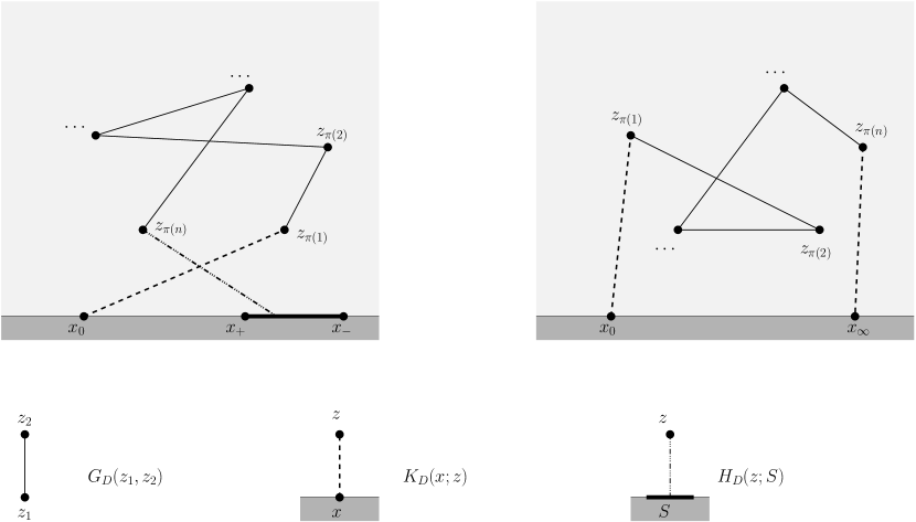
Figure 1: Example diagrams representing the terms in the local time multipoint correlation functions. Dipolar case (15) is on the left and chordal case (16) on the right.

with explicit expressions

$$G_{\mathbb{H}}(z,w) = -\frac{1}{\pi}\log\big{|}\frac{z-w}{z-\overline{w}}\big{|}$$

$$K_{\mathbb{H}}({x_{0}},z) = -\frac{2}{\pi}\;\Im\textrm{m }\big{(}\frac{1}{z-{x_{0}}}\big{)}$$

$$H_{\mathbb{H}}(z,[x_{+},x_{-}]) = \frac{1}{\pi}\;\Im\textrm{m }\Big{(}\log\frac{z-x_{-}}{z-x_{+}}\Big{)}\textrm{ .}$$

It is convenient to represent the terms in this result diagrammatically as in figure 1. The chordal case is obtained by limit $\delta^{\prime}\rightarrow 0$ with choice $x_{\pm}={x_{\infty}}\mp\delta^{\prime}$,

$$C^{{x_{0}};{x_{\infty}}}(z_{1},\ldots,z_{n})$$ (16)

$$:= \lim_{\delta\rightarrow 0}\frac{1}{\delta\,\delta^{\prime}}\mathsf{E}_{\mathrm{BM}}^{{x_{0}}+i\delta}\Big{[}\ell(z_{1})\cdots\ell(z_{n})\;\mathbf{1}_{{\bf{B}}_{\tau_{D}}\in[{x_{\infty}}-\delta^{\prime},{x_{\infty}}+\delta^{\prime}]}\Big{]}$$

$$= \sum_{\pi\in S_{n}}K_{\mathbb{H}}({x_{0}},z_{\pi(1)})\;\Big{(}\prod_{j=2}^{n}G_{\mathbb{H}}(z_{\pi(j-1)},z_{\pi(j)})\Big{)}\;K_{\mathbb{H}}({x_{\infty}},z_{\pi(n)})\textrm{ .}$$

5.2 On conformal field theory of LERWs

It is known from general arguments that SLE_κ corresponds to conformal field theory of central charge $c=\frac{(6-\kappa)(3\kappa-8)}{2\kappa}$, [2], so that LERWs should have $c=-2$. But we can be more specific about the CFT appropriate for our case.

First of all, LERWs are “dual” to uniform spanning trees (UST) [30, 26, 19], for which fermionic field theories have been given [9], see also [23]. Indeed a field theory of free symplectic fermions would have central charge $c=-2$, [13]. The theory is Gaussian. It has two basic fields $\chi^{+}$ and $\chi^{-}$ whose correlation functions in domain $\mathbb{D}$ (Dirichlet boundary conditions) are determined by

$$\langle\chi^{\alpha}(z,\overline{z})\chi^{\beta}(w,\overline{w})\rangle=J^{\alpha\beta}G_{\mathbb{D}}(z,w)\textrm{ ,}$$

with $J^{++}=0=J^{--}$, $J^{+-}=1=-J^{-+}$, and the Wick’s formula.

The fields $\chi^{\alpha}(z,\overline{z})$ are fermionic but scalars, meaning that they transform like scalars under conformal transformations. We shall also be interested in the composite operator $\,\mathrm{:}\chi^{-}\chi^{+}\mathrm{:}\,$ which has to be defined via a point splitting to remove the short distance singularity

$$\;\,\mathrm{:}\chi^{-}\,\chi^{+}\mathrm{:}\,(z,\overline{z})=\lim_{z\to w}\;\chi^{-}(z,\overline{z})\,\chi^{+}(w,\overline{w})-\frac{1}{2\pi}\log|z-w|^{2}$$

Due to this regularisation, $\,\mathrm{:}\chi^{-}\chi^{+}\mathrm{:}\,$ transforms with a logarithmic anomaly under conformal transformations:

$$\,\mathrm{:}\chi^{-}\,\chi^{+}\mathrm{:}\,(z,\overline{z})\to\,\mathrm{:}\chi^{-}\,\chi^{+}\mathrm{:}\,(g(z),\overline{g(z)})-\frac{1}{2\pi}\log|g^{\prime}(z)|^{2}\textrm{ .}$$ (17)

The stress tensor is $T(z)=2\pi\;\,\mathrm{:}\partial_{z}\chi^{+}(z,\overline{z})\,\partial_{z}\chi^{-}(z,\overline{z})\mathrm{:}\,$ with the normal ordering defined by a point splitting similar as above. It is easy to verify that both operators $\partial_{z}\chi^{\alpha}$ are operators of dimension $1$ satisfying the level two null vector equation $(L_{-2}-1/2L_{-1}^{2})\partial_{z}\chi^{\alpha}=0$ with $L_{n}$, $T(z)=\sum_{n}L_{n}z^{-n-2}$, the Virasoro generators. It is this equation which helps identifying the symplectic fermions as the CFT associated to LERW. We will be able to identify some other fields with natural LERW quantities, although there are some important ones for which a good understanding is still lacking (to us).

5.2.1 Boundary changing operators

The partition functions without perturbation involve only boundary operators that account for the LERW starting from ${x_{0}}\in\mathbb{R}$ and aiming at $S\subset\mathbb{R}$. We will identify them below.

We consider the symplectic fermion field theory in the upper half plane $\mathbb{H}$. Let us define the boundary fields $\psi^{\pm}$ as normal derivatives of $\chi^{\pm}$ on the real axis

$$\psi^{\pm}({x_{0}})=\lim_{\delta\rightarrow 0}\frac{1}{\delta}\chi^{\pm}({x_{0}}+i\delta,{x_{0}}-i\delta)\textrm{ .}$$

The level two null field equation says the fields $\psi^{+}$ and $\psi^{-}$ can account for starting point and end point of SLE₂ curves [2, 4, 6] (see also section 5.2.3). And indeed, the two point function $\langle\psi^{+}({x_{0}})\psi^{-}({x_{\infty}})\rangle=\frac{2}{\pi}({x_{\infty}}-{x_{0}})^{-2}$ reproduces our partition function in the chordal setup, compare with sections 3 and 5.1.1.

Let us then remark that the dipolar LERW from ${x_{0}}$ to $[x_{+},x_{-}]$, conditioned to hit a point ${x_{\infty}}\in[x_{+},x_{-}]$ is just the chordal LERW from ${x_{0}}$ to ${x_{\infty}}$ as follows directly from the definitions. It has been pointed out in [5] that $\kappa=2$ is the only value for which the corresponding property holds for dipolar and chordal SLE_κ.

Following the above remark, we decompose the dipolar probability measure according to the endpoint ${x_{\infty}}\in[x_{+},x_{-}]$

$$\mathsf{P}_{{x_{0}},[x_{+},x_{-}]}^{0}\;=\;\int_{x_{+}}^{x_{-}}\mathrm{d}{x_{\infty}}\,A({x_{\infty}})\mathsf{P}^{0}_{{x_{0}};{x_{\infty}}}\textrm{ ,}$$

where $A$ is the probability density for LERW to end at ${x_{\infty}}$

$$A({x_{\infty}}) \;=\; \lim_{\delta,\delta^{\prime}\downarrow 0}\frac{\frac{1}{2\delta^{\prime}}\;H({x_{0}}+i\delta;[{x_{\infty}}-\delta^{\prime},{x_{\infty}}+\delta^{\prime}])}{H({x_{0}}+i\delta);[x_{+},x_{-}])}\;=\;\frac{\frac{1}{2}Z^{{x_{0}};{x_{\infty}}}}{Z^{{x_{0}};[x_{+},x_{-}]}_{0}}$$ (18)

$$\;=\; \frac{({x_{0}}-x_{-})({x_{0}}-x_{+})}{(x_{-}-x_{+})({x_{\infty}}-{x_{0}})^{2}}\textrm{ .}$$

As this is just a ratio of the correlation functions, we may say that the dipolar boundary changing operators are $\psi^{+}({x_{0}})$ and $\frac{1}{2}\int_{x_{+}}^{x_{-}}\psi^{-}({x_{\infty}})\,\mathrm{d}{x_{\infty}}$. Indeed, the partition function is reproduced by

$$\langle\psi^{+}({x_{0}})\,\big{(}\frac{1}{2}\int_{x_{+}}^{x_{-}}\psi^{-}({x_{\infty}})\;\mathrm{d}{x_{\infty}}\big{)}\rangle\;=\;\frac{1}{\pi}\frac{x_{-}-x_{+}}{(x_{-}-{x_{0}})(x_{+}-{x_{0}})}\;=\;Z^{{x_{0}};[x_{+},x_{-}]}_{0}\textrm{ .}$$

5.2.2 Field theory representation of Brownian local time

In section 5.1.3 we derived the expressions (15) and (16) for Brownian local time correlations. We recall that in the chordal case, the multipoint correlation function in the upper half plane is

$$C^{{x_{0}};{x_{\infty}}}(z_{1},\ldots,z_{n})$$

$$= \sum_{\pi\in S_{n}}K_{\mathbb{H}}({x_{0}},z_{\pi(1)})\;\Big{(}\prod_{j=2}^{n}G_{\mathbb{H}}(z_{\pi(j-1)},z_{\pi(j)})\Big{)}\;K_{\mathbb{H}}({x_{\infty}},z_{\pi(n)})\textrm{ .}$$

The two point functions of symplectic fermions involve the same building blocks $\langle\chi^{+}(z)\chi^{-}(w)\rangle=G_{\mathbb{H}}(z,w)$ and $\langle\psi^{+}(x)\chi^{-}(z)\rangle=\langle\chi^{+}(z)\psi^{-}(x)\rangle=K_{\mathbb{H}}(x;z)$. Thus the formula is clearly reminiscent of what Wick’s formula gives for correlations of the composite operator

$$\,\mathrm{:}\chi^{-}\chi^{+}\mathrm{:}_{\mathbb{D}}\,(z)=\lim_{z^{\prime},z^{\prime\prime}\rightarrow z}\Big{(}\chi^{-}(z^{\prime})\chi^{+}(z^{\prime\prime})-G_{\mathbb{D}}(z^{\prime},z^{\prime\prime})\Big{)}\textrm{ ,}$$ (19)

where we substract the full two point function in domain $\mathbb{D}$ so that in the Wick’s formula no terms with pairing within normal orderings appear. Inserting also the boundary changing operators $\psi^{+}({x_{0}})$ and $\psi^{-}({x_{\infty}})$ for the chordal case, we get

$$\langle\psi^{+}({x_{0}})\;\,\mathrm{:}\chi^{-}\chi^{+}\mathrm{:}_{\mathbb{H}}\,(z_{1})\;\cdots\;\,\mathrm{:}\chi^{-}\chi^{+}\mathrm{:}_{\mathbb{H}}\,(z_{n})\;\psi^{-}({x_{\infty}})\rangle$$

$$= \sum_{\begin{subarray}{c}J\subset\{1,\ldots,n\},\;\pi\in S_{J}\\ J_{1},\ldots,J_{s}\textrm{ partition of }\complement J\\ \textrm{$\pi_{r}$ cyclic ordering of $J_{r}$, $r=1,\ldots,s$}\end{subarray}}\prod_{r=1}^{s}\Big{(}G_{\mathbb{H}}(z_{\pi_{r}(1)},z_{\pi_{r}(2)})\cdots G_{\mathbb{H}}(z_{\pi_{r}(|J_{r}|)},z_{\pi_{r}(1)})\Big{)}$$

$$\qquad\times\Big{(}K_{\mathbb{H}}({x_{0}},z_{\pi}(1))\big{(}\prod_{j=2}^{|J|}G_{\mathbb{H}}(z_{\pi(j-1)},z_{\pi(j)})\big{)}K_{\mathbb{H}}({x_{\infty}},z_{\pi(|J|)})\Big{)}\textrm{ ,}$$

which is represented diagrammatically in figure 2.

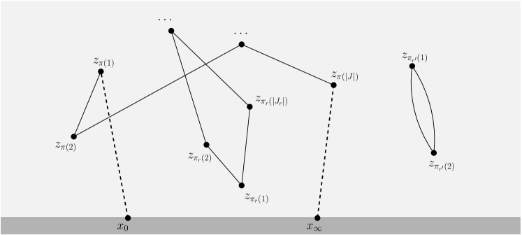
Figure 2: Example diagram for a term appearing in the correlation function (5.2.2) of fields $\,\mathrm{:}\chi^{-}\chi^{+}\mathrm{:}_{\mathbb{H}}\,$. The component containing boundary points $x_{0}$ and $x_{\infty}$ corresponds to $J$ whereas the rest of the connected components correspond to $J_{1},\ldots,J_{s}$. Within each component $J_{r}$ we sum over inequivalent cyclic orderings $\pi_{r}$ of it.

The terms with $J=\{1,2,\ldots,n\}$ are what appear in the correlation function (16) and what are illustrated in figure 1, the rest of the terms correspond to disconnected diagrams. To cure this, we must divide out a loop soup contribution that cancels the disconnected diagrams. We indeed have

$$Z^{{x_{0}};{x_{\infty}}}_{\nu} = \lim_{\delta\rightarrow 0}\frac{1}{\delta\,\delta^{\prime}}\mathsf{E}^{{x_{0}}+i\delta}_{\mathrm{BM}}\Big{[}e^{-\varepsilon\int_{\mathbb{H}}\tilde{\nu}(z)\ell(z)\;\mathrm{d}^{2}z}\;\mathbf{1}_{{\bf{B}}_{\tau_{\mathbb{H}}}\in[{x_{\infty}}-\delta^{\prime},{x_{\infty}}+\delta^{\prime}]}\Big{]}$$

$$= \frac{\langle\psi^{+}({x_{0}})\;e^{-\varepsilon\int_{\mathbb{H}}\tilde{\nu}(z)\,\mathrm{:}\chi^{-}\chi^{+}\mathrm{:}_{\mathbb{H}}\,(z)\;\mathrm{d}^{2}z}\;\psi^{-}({x_{\infty}})\rangle}{\langle e^{-\varepsilon\int_{\mathbb{H}}\tilde{\nu}(z)\,\mathrm{:}\chi^{-}\chi^{+}\mathrm{:}_{\mathbb{H}}\,(z)\;\mathrm{d}^{2}z}\rangle}$$

in the sense of formal expansion in powers of $\varepsilon$. In this formula, however, the precise normal ordering prescription of $\chi^{-}\chi^{+}$ doesn’t matter: had we made another substraction of the logarithmic divergence, the result would differ by a constant and would cancel in the ratio

$$Z^{{x_{0}};{x_{\infty}}}_{\nu} = \frac{\langle\psi^{+}({x_{0}})\;e^{-\varepsilon\int_{\mathbb{H}}\tilde{\nu}(z)\,\mathrm{:}\chi^{-}\chi^{+}\mathrm{:}\,(z)\;\mathrm{d}^{2}z}\;\psi^{-}({x_{\infty}})\rangle}{\langle e^{-\varepsilon\int_{\mathbb{H}}\tilde{\nu}(z)\,\mathrm{:}\chi^{-}\chi^{+}\mathrm{:}\,(z)\;\mathrm{d}^{2}z}\rangle}\textrm{ ,}$$ (21)

so in particular we may use the ordinary normal ordering prescription.

From the chordal case formulas (16) and (21) we can immediately derive also a CFT formula for the dipolar case by observing that $\int_{x_{+}}^{x_{-}}K_{\mathbb{H}}({x_{\infty}},z)\;\mathrm{d}{x_{\infty}}=2\,H_{\mathbb{H}}(z;[x_{+},x_{-}])$. This reads

$$Z^{{x_{0}};[x_{+},x_{-}]}_{\nu} = \frac{\langle\psi^{+}({x_{0}})\;e^{-\varepsilon\int_{\mathbb{H}}\tilde{\nu}(z)\,\mathrm{:}\chi^{-}\chi^{+}\mathrm{:}\,(z)\;\mathrm{d}^{2}z}\;\big{(}\frac{1}{2}\int_{x_{+}}^{x_{-}}\psi^{-}({x_{\infty}})\;\mathrm{d}{x_{\infty}}\big{)}\rangle}{\langle e^{-\varepsilon\int_{\mathbb{H}}\tilde{\nu}(z)\,\mathrm{:}\chi^{-}\chi^{+}\mathrm{:}\,(z)\;\mathrm{d}^{2}z}\rangle}\textrm{ .}$$

5.2.3 SLE martingales from conformal field theory

By a two step averaging argument one can construct tautological martingales for growth processes describing random curves, see for example [4, 6]. One splits the full statistical average to average over configurations that produce a given initial segment of a curve $\gamma[0,t]$, which is then still to be averaged over all possible initial segments. The information about the initial segment is precisely what the SLE filtration $\mathcal{F}_{t}$ represents. If the statistical average can be replaced by CFT correlation function in the continuum limit, one concludes that for any CFT field $\mathcal{O}$ (e.g. product of several primary fields $\mathcal{O}=\Phi_{\alpha_{1}}(z_{1},\overline{z}_{1})\cdots\Phi_{\alpha_{n}}(z_{n},\overline{z}_{n})$) the ratio

$$\frac{{\langle\mathcal{O}\;(\mathrm{bdry}\;\mathrm{cond.})\rangle}_{\mathbb{H}_{t}}}{{\langle(\mathrm{bdry}\;\mathrm{cond.})\rangle}_{\mathbb{H}_{t}}}$$

is a martingale, where $\langle\cdots({\mathrm{bdry}\;\mathrm{cond.}})\rangle_{\mathbb{H}_{t}}$ represents CFT expectation in domain $\mathbb{H}_{t}=\mathbb{H}\setminus\gamma[0,t]$ with insertions of boundary changing operators to account for the boundary conditions. In the denominator, the expected value of the boundary operators corresponds to the partition function. We emphasize that the operator $\mathcal{O}$ is constant in time — time dependency arises only through the changing domain $\mathbb{H}_{t}$ and the operator placed at the tip $\gamma_{t}$ of the curve. For example attempting to use $\mathcal{O}=\,\mathrm{:}\chi^{-}\chi^{+}\mathrm{:}\,_{\mathbb{H}_{t}}$ (the closest analog in field theory of the local time $\ell(z)$) will not result in a (local) martingale because the normal ordering (subtraction) is time dependent.

The above argument has a converse, too. If one considers SLE variant with driving process $\mathrm{d}\xi_{t}=\sqrt{\kappa}\;\mathrm{d}B_{t}+\partial_{\xi}\log Z_{\mathbb{H}}\;\mathrm{d}t$ and uses transformation properties of CFT fields, then by a direct check one concludes that ratios $\langle\mathcal{O}\rangle^{\mathrm{bdry}\;\mathrm{cond.}}/Z$ are local martingales provided the boundary changing operators include a field $\psi$ at the tip $\gamma_{t}$ that has a vanishing descendant $(-4\,L_{-2}+\kappa\,L_{-1}^{2})\psi=0$.

For the continuum limit of chordal and dipolar LERWs we have identified the appropriate boundary changing operators in section 5.2.1 and therefore the ratios

$$\frac{\langle\mathcal{O}\;\psi^{+}(\gamma_{t})\,\psi^{-}({x_{\infty}})\rangle_{\mathbb{H}_{t}}}{\langle\psi^{+}(\gamma_{t})\,\psi^{-}({x_{\infty}})\rangle_{\mathbb{H}_{t}}} \frac{\langle\mathcal{O}\;\psi^{+}(\gamma_{t})\;\int_{x_{+}}^{x_{-}}\psi^{-}({x_{\infty}})\,\mathrm{d}{x_{\infty}}\rangle_{\mathbb{H}_{t}}}{\langle\psi^{+}(\gamma_{t})\;\int_{x_{+}}^{x_{-}}\psi^{-}({x_{\infty}})\,\mathrm{d}{x_{\infty}}\rangle_{\mathbb{H}_{t}}}$$ and

should produce martingales in the two cases respectively. We will in particular be interested in inserting the perturbing operator $\,\mathrm{:}\chi^{-}\chi^{+}\mathrm{:}\,(z)$, since to first order the correlation functions in presence of the perturbation are given by extra insertion of $\mathcal{O}=(\mathbf{1}-\varepsilon\int_{\mathbb{H}}\tilde{\nu}(z)\,\mathrm{:}\chi^{-}\chi^{+}\mathrm{:}\,(z)\;\mathrm{d}^{2}z)$.

In the half-plane Wick’s theorem gives the result

$$\frac{1}{2}\;\langle\,\mathrm{:}\chi^{-}\chi^{+}\mathrm{:}_{\mathbb{H}}\,(z)\;\psi^{+}(\gamma_{t})\;\int_{x_{+}}^{x_{-}}\psi^{-}({x_{\infty}})\,\mathrm{d}{x_{\infty}}\rangle_{\mathbb{H}} \;=\; K_{\mathbb{H}}({x_{0}};z)\,H_{\mathbb{H}}(z;[x_{+},x_{-}])$$

which we recognize also as the local time correlation function $C^{{x_{0}};[x_{+},x_{-}]}(z)$, because the one point function has no disconnected diagrams. Recall the logarithmic anomaly in the transformation property of $\,\mathrm{:}\chi^{-}\chi^{+}\mathrm{:}\,(z)$, eq.(17) to get

$$N_{t}^{{x_{0}};[x_{+},x_{-}]}(z)\;=\;\frac{\langle\,\mathrm{:}\chi^{-}\chi^{+}\mathrm{:}\,(z)\;\psi^{+}(\gamma_{t})\;\int_{x_{+}}^{x_{-}}\psi^{-}({x_{\infty}})\,\mathrm{d}{x_{\infty}}\rangle_{\mathbb{H}_{t}}}{\langle\psi^{+}(\gamma_{t})\;\int_{x_{+}}^{x_{-}}\psi^{-}({x_{\infty}})\,\mathrm{d}{x_{\infty}}\rangle_{\mathbb{H}_{t}}}$$ (22)

$$\;=\; \frac{\langle\Big{(}\,\mathrm{:}\chi^{-}\chi^{+}\mathrm{:}\,(g_{t}(z))+\frac{1}{\pi}\log|g^{\prime}_{t}(z)|\Big{)}\;\psi^{+}(\xi_{t})\;\int_{X^{+}_{t}}^{X^{-}_{t}}\psi^{-}({x_{\infty}})\,\mathrm{d}{x_{\infty}}\rangle_{\mathbb{H}}}{\langle\psi^{+}(\xi_{t})\;\int_{X^{+}_{t}}^{X^{-}_{t}}\psi^{-}({x_{\infty}})\,\mathrm{d}{x_{\infty}}\rangle_{\mathbb{H}}}$$

$$\;=\; -\frac{1}{\pi}\log\frac{2\;\Im\textrm{m }(g_{t}(z))}{|g_{t}^{\prime}(z)|}+\frac{K_{\mathbb{H}}(\xi_{t};g_{t}(z))\,H_{\mathbb{H}}(g_{t}(z);[X^{+}_{t},X^{-}_{t}])}{Z_{0}^{\xi_{t};[X^{+}_{t},X^{-}_{t}]}}\textrm{ ,}$$

where $X^{\pm}_{t}=g_{t}(x_{\pm})$. The process $N_{t}(z)$ should be a local martingale by construction and one can indeed verify this directly by Itô’s formula.

The formula (22) has a natural probabilistic interpretation, too: as a conditional expected value of the local time of the underlying random walk at $z$. The two parts correspond to the splitting $\ell_{\mathbb{H}}=\ell_{\mathbb{H}\setminus\gamma[0,t]}+\ell^{(t)}_{\mathbb{H}}$. The second term is indeed, by conformal invariance of the local time $\ell(z)$, just the expected value of the local time of Brownian motion in $\mathbb{H}\setminus\gamma[0,t]$ started from $\gamma_{t}$ and conditioned to exit through $[x_{+},x_{-}]$. The first term is $A_{t}=-\frac{1}{\pi}\log\rho_{\mathbb{H}_{t}}(z)$, where $\rho_{\mathbb{H}_{t}}(z)=\frac{2\,\Im\textrm{m }(g_{t}(z))}{|g_{t}^{\prime}(z)|}$ is the conformal radius of $z$ in $\mathbb{H}\setminus\gamma[0,t]$. In particular the first term is an increasing process. Recall that in the discrete setup, conditional on loop erasure producing a given initial segment of the curve, the second term corresponds to the expected local time at $z$ of the underlying random walk after its last visit to the tip of the curve, see [19] whereas the first part, more precisely $A_{t}-A_{0}$, should be interpreted as the expected local time at $z$ of the (erased) loops until the last visit to the tip. The fact that $A_{t}$ is increasing is then natural since as time increases we erase more loops. Seen this way, $A_{t}-A_{0}$ is also what we called the (nonlocal) interface energy of the LERW in section 4.2.2.

It has been argued [20] that it should be possible to add to SLE₂ Brownian bubbles so as to reconstruct the underlying Brownian motion. We notice indeed that

$$A_{t}-A_{0}=\frac{4}{\pi}\;\int_{0}^{t}\frac{\big{(}\Im\textrm{m }g_{s}(z)\big{)}^{2}}{|g_{s}(z)-\xi_{s}|^{4}}\;\mathrm{d}s\textrm{ ,}$$

where the integrand is morally twice the “expected” local time at $z$ of a Browian bubble in $\mathbb{H}\setminus\gamma[0,s]$ from $\gamma_{s}$. Actually Brownian bubbles don’t form a probability measure but an infinite measure. If we normalize it as in [20] (but we must not forget about the time parametrization of the bubbles, see [22]), the integral with respect to the bubble measure of the local time is $\frac{\pi}{2}K(\xi_{s};g_{s}(z))^{2}=\frac{2}{\pi}\big{(}\Im\textrm{m }g_{s}(z)/|g_{s}(z)-\xi_{s}|^{2}\big{)}^{2}$. The factor two is an intensity at which we need to add the bubbles to the curve — it is minus the central charge, $\lambda=-c=2$.

In the chordal case we obtain similar formulas — in fact they can also be recovered by limit of the dipolar case. For the record, we give the (local) martingale

$$N_{t}^{{x_{0}};{x_{\infty}}}(z) \;=\; -\frac{1}{\pi}\log\frac{2\;\Im\textrm{m }(g_{t}(z))}{|g_{t}^{\prime}(z)|}+\frac{K_{\mathbb{H}}(\xi_{t};g_{t}(z))\,K_{\mathbb{H}}(\eta_{t};g_{t}(z))}{Z_{0}^{\xi_{t};\eta_{t}}}\textrm{ ,}$$

where $\eta_{t}=g_{t}({x_{\infty}})$. It is in particular worth noticing that the “expected local time of the erased loops” $A_{t}-A_{0}$ has the same formula and depends only on the shape of the “initial segment of the loop-erasure” $\gamma[0,t]$.

5.3 Off-critical LERW and massive symplectic fermions

The conformal field theory of LERW is the symplectic fermion theory with central charge $c=-2$. As we have argued when defining the scaling limit of the LERW, going off-criticality amounts to perturbing by an operator of scaling dimension $0$. In terms of Brownian motion the off-critical weighting is given by the local time which is closely linked to the composite operator $:\chi^{-}\chi^{+}:$ as we’ve shown above, cf. eq.(21) and $N_{t}(z)$ in section 5.2.3. In fact, as the perturbing field is $:\chi^{+}\chi^{-}:$ and the action for the off-critical theory thus reads

$$(const.)\int_{\mathbb{H}}d^{2}z[J_{\alpha\beta}\bar{\partial}\chi^{\alpha}\partial\chi^{\beta}+8\nu(z)\,J_{\alpha\beta}\chi^{\alpha}\chi^{\beta}],$$

the need to divide by $\langle e^{-\int\nu(z)\,\mathrm{:}\chi^{-}\chi^{+}\mathrm{:}\,(z)\;\mathrm{d}^{2}z}\rangle$ stems just from the normalization of the new measure. We remark in particular that the off-critical theory is still Gaussian with two point function

$$\langle\chi^{\alpha}(z,\overline{z})\chi^{\beta}(w,\overline{w})\rangle_{\nu}=J^{\alpha\beta}G^{\nu}_{\mathbb{H}}(z,w)\textrm{ ,}$$

where $(-\nu(w)+\frac{1}{2}\triangle_{w})G^{\nu}_{\mathbb{H}}(z,w)=-2\delta(z-w)$.

For simplicity we look at the theory in the upper half plane. The boundary conditions are identical to that of the critical theory.

Suppose, as has been argued, that the off-critical measure $\mathsf{P}^{\nu}_{\mathbb{H}}$ on curves differs from the critical one by a Radon-Nikodym derivative $M_{t}$ given by (6). We have been able to compute the limit of partition functions in (14) & (15) or alternatively in (21), and we know that the energy term $\Delta{\cal E}_{\mathbb{H}}(\gamma[0,t])$ is monotone in $t$, thus of finite variation (can not have a $\mathrm{d}B_{t}$ like increment). This is in fact enough to determine what the energy term is in our case: it must compensate the drift so that $M_{t}$ becomes a martingale and it is not difficult to check that this requires

$$e^{\Delta{\cal E}_{\mathbb{H}}(\gamma[0,t])}\;=\; \frac{\big{\langle}\exp\big{(}-\int\mathrm{d}^{2}z\;\nu(z)\,\mathrm{:}\chi^{-}\chi^{+}\mathrm{:}_{\mathbb{H}}\,(z)\big{)}\;(\mathrm{bdry}\;\mathrm{cond.})\big{\rangle}_{\mathbb{H}_{t}}}{\big{\langle}\exp\big{(}-\int\mathrm{d}^{2}z\;\nu(z)\,\mathrm{:}\chi^{-}\chi^{+}\mathrm{:}\,_{\mathbb{H}_{t}}(z)\big{)}\;(\mathrm{bdry}\;\mathrm{cond.})\big{\rangle}_{\mathbb{H}_{t}}}$$

$$=\; \exp\Big{(}-\frac{1}{\pi}\int\mathrm{d}^{2}z\;\nu(z)\;\log\big{(}\frac{\rho_{\mathbb{H}_{t}}(z)}{\rho_{\mathbb{H}}(z)}\big{)}\Big{)}\textrm{ .}$$ (23)

The change in interface energy is therefore given by the bubble soup $A_{t}-A_{0}$ as we could have expected. Furthermore and importantly, the field theoretic formula (7) for $M_{t}$ to first order holds with $\Phi(z)=\,\mathrm{:}\chi^{-}\chi^{+}\mathrm{:}\,(z)$.

5.3.1 Subinterval hitting probability from field theory

We will now show how to use the field theory interpretation to compute probabilities for the off-critical LERW. We work in the dipolar setup, a LERW from ${x_{0}}$ to $[x_{+},x_{-}]$ in $\mathbb{H}$, and ask what is the probability for the endpoint of the LERW to be on a subinterval $S=[x^{\prime}_{+},x^{\prime}_{-}]\subset[x_{+},x_{-}]$. In the next section we derive the same result from direct probabilistic considerations.

From Boltzmann rules, this probability is the ratio of two partition functions: the partition of LERW exiting on $[x^{\prime}_{+},x^{\prime}_{-}]$ by that of LERW exiting on $[x_{+},x_{-}]$. In field theory this becomes the ratio of two correlation functions but with different boundary conditions (or equivalently, insertion of boundary changing operators at different locations). Hence, this hitting probability is expected to be:

$$\mathsf{P}^{\nu}_{\xi_{0};[x_{+},x_{-}]}\Big{[}\textrm{end in $[x^{\prime}_{+},x^{\prime}_{-}]$}\Big{]}=\frac{\langle\psi^{+}(\xi_{0})\,\frac{1}{2}\big{(}\int_{x^{\prime}_{+}}^{x^{\prime}_{-}}\psi^{-}({x_{\infty}})\mathrm{d}{x_{\infty}}\big{)}\rangle_{\nu}}{\langle\psi^{+}(\xi_{0})\,\frac{1}{2}\big{(}\int_{x_{+}}^{x_{-}}\psi^{-}({x_{\infty}})\mathrm{d}{x_{\infty}}\big{)}\rangle_{\nu}}$$

where the operator $\psi^{+}(\xi_{0})$ is the operator which creates the LERWs and the operator $\frac{1}{2}\int_{x^{\prime}_{+}}^{x^{\prime}_{-}}\psi^{-}(x_{\infty})\,\mathrm{d}x_{\infty}$ or $\frac{1}{2}\int_{x_{+}}^{x_{-}}\psi^{-}(x_{\infty})\,\mathrm{d}x_{\infty}$ are those conditioning the curves to stop on the interval $[x^{\prime}_{+},x^{\prime}_{-}]$ or $[x_{+},x_{-}]$, so that they impose the boundary conditions.

At criticality, the correlation function $\langle\psi^{+}(\xi_{0})\,\frac{1}{2}\int_{x^{\prime}_{+}}^{x^{\prime}_{-}}\psi^{-}(x_{\infty})\,\mathrm{d}x_{\infty}\rangle_{0}$ is computable from the limit behavior of the harmonic measure $H_{\mathbb{H}}(z_{0},[x^{\prime}_{+},x^{\prime}_{-}])$ as $z_{0}\to\xi_{0}$ so that

$$\langle\psi^{+}(\xi_{0})\,\big{(}\int_{x^{\prime}_{+}}^{x^{\prime}_{-}}\psi^{-}({x_{\infty}})\mathrm{d}{x_{\infty}}\big{)}\rangle_{0}=\frac{2}{\pi}\frac{(x^{\prime}_{-}-x^{\prime}_{+})}{(\xi_{0}-x^{\prime}_{-})(\xi_{0}-x^{\prime}_{+})}\textrm{ .}$$

The hitting probability in $\mathbb{H}$ at the conformal point is thus

$$\mathsf{P}^{0}_{\xi_{0};[x_{+},x_{-}]}\Big{[}\textrm{end in $[x^{\prime}_{+},x^{\prime}_{-}]$}\Big{]}=\frac{(x^{\prime}_{-}-x^{\prime}_{+})(\xi_{0}-x_{-})(\xi_{0}-x_{+})}{(x_{-}-x_{+})(\xi_{0}-x^{\prime}_{-})(\xi_{0}-x^{\prime}_{+})}.$$

Off-criticality, the correlation functions $\langle\psi^{+}(\xi_{0})\,\frac{1}{2}\big{(}\int_{x^{\prime}_{+}}^{x^{\prime}_{-}}\psi^{-}({x_{\infty}})\mathrm{d}{x_{\infty}}\big{)}\rangle_{\nu}$ are computable via the limiting behavior of $\langle\chi^{+}(z_{0})\,\frac{1}{2}\big{(}\int_{x^{\prime}_{+}}^{x^{\prime}_{-}}\psi^{-}({x_{\infty}})\mathrm{d}{x_{\infty}}\big{)}\rangle_{\nu}$ with $z\in\mathbb{H}$ but approaching the real axis, $z\to\xi_{0}$. The off-critical probability is thus expected to be

$$\mathsf{P}^{\nu}_{\xi_{0};[x_{+},x_{-}]}\Big{[}\textrm{end in $[x^{\prime}_{+},x^{\prime}_{-}]$}\Big{]}=\lim_{z\to\xi_{0}}\frac{\Gamma^{\nu}_{\mathbb{H},[x^{\prime}_{+},x^{\prime}_{-}]}(z)}{\Gamma^{\nu}_{\mathbb{H},[x_{+},x_{-}]}(z)}$$ (24)

with $\Gamma^{\nu}_{\mathbb{H},[x^{\prime}_{+},x^{\prime}_{-}]}(z)$ solution of $(-\nu(z)+\frac{1}{2}\triangle_{z})\Gamma^{\nu}_{\mathbb{H},[x^{\prime}_{+},x^{\prime}_{-}]}(z)=0$. To find the boundary conditions observe that the leading term in the OPE $\chi^{+}(z)\psi^{-}({x_{\infty}})\sim\frac{-2}{\pi}\Im\textrm{m }\big{(}\frac{1}{z-{x_{\infty}}}\big{)}$ remains unchanged in the off-critical theory. One finds that $\Gamma^{\nu}_{\mathbb{H},[x^{\prime}_{+},x^{\prime}_{-}]}(z)\to 1$ for $z\to(x^{\prime}_{+},x^{\prime}_{-})$ and $\Gamma^{\nu}_{\mathbb{H},[x^{\prime}_{+},x^{\prime}_{-}]}(z)\to 0$ for $z\to\mathbb{R}\setminus[x^{\prime}_{+},x^{\prime}_{-}]$. Both $\Gamma^{\nu}_{\mathbb{H},[x^{\prime}_{+},x^{\prime}_{-}]}$ and $\Gamma^{\nu}_{\mathbb{H},[x_{+},x_{-}]}$ vanish at $\xi_{0}\in\mathbb{R}\setminus[x_{+},x_{-}]$, but their ratio tends to a finite limit.

In the following section, we shall present a probabilistic derivation of this field theory inspired formula.

5.3.2 Probabilistic derivation of subinterval hitting probability

Above we gave a field theory flavoured discussion of the probability that a perturbed LERW in $\mathbb{H}$ from ${x_{0}}$ to $[x_{+},x_{-}]$ ends on a subinterval $[x^{\prime}_{+},x^{\prime}_{-}]\subset[x_{+},x_{-}]$. It is easy to justify the formulas obtained there by computations with Brownian motion.

Most importantly, we notice that the question of endpoint is a property of the (weighted) random walk $W$ that we then decided to loop erase. Indeed, by construction the loop erasing procedure doesn’t change the starting point and end point. Therefore we only need to find the subinterval hitting probability of the weighted random walk, which in the continuum boils down to a Brownian motion computation.

We thus consider a walk in the upper half plane, started from $x_{0}\in\mathbb{R}$ (or an approximation to it) and conditioned to exit the half plane through $[x_{+},x_{-}]\subset\mathbb{R}$ (a lattice approximation of it). The walk $(W^{(a)}_{j})_{j=0}^{\tau_{\mathbb{H}^{(a)}}}$ is weighted by $\exp(-\sum_{j}a^{2}\nu^{(a)}(W^{(a)}_{j}))$ relative to the symmetric random walk, so the probability of an event $E$ is

$$\mathsf{P}^{\nu}_{w;[x_{+},x_{-}]}[E]\;=\;\frac{\mathsf{E}^{w}_{\mathrm{RW}}\big{[}\mathbf{1}_{E\,\cap\,\{W^{(a)}_{\tau_{\mathbb{H}^{(a)}}}\in[x_{+},x^{-}]\}}\;\exp(-\sum_{j}a^{2}\nu^{(a)}(W^{(a)}_{j}))\big{]}}{\mathsf{E}^{w}_{\mathrm{RW}}\big{[}\mathbf{1}_{W^{(a)}_{\tau_{\mathbb{H}^{(a)}}}\in[x_{+},x^{-}]}\;\exp(-\sum_{j}a^{2}\nu^{(a)}(W^{(a)}_{j}))\big{]}}\textrm{ .}$$

Take $E$ to be the event $W^{(a)}_{\tau_{\mathbb{H}^{(a)}}}\in[x^{\prime}_{+},x^{\prime}_{-}]\subset[x_{+}x_{-}]$. The continuum limit $a\downarrow 0$ of the probability of exiting through $[x^{\prime}_{+},x^{\prime}_{-}]\subset[x_{+},x_{-}]$ is then computed using Brownian motion

$$\mathsf{P}^{\nu}_{w;[x_{+},x_{-}]}\big{[}\textrm{end in $[x^{\prime}_{+},x^{\prime}_{-}]$}\big{]} = \frac{\mathsf{E}_{\mathrm{BM}}^{w}[e^{-\int\nu({\bf{B}}_{s})\mathrm{d}s}\;\mathbf{1}_{{\bf{B}}_{\tau_{\mathbb{H}}}\in[x^{\prime}_{+},x^{\prime}_{-}]}]}{\mathsf{E}_{\mathrm{BM}}^{w}[e^{-\int\nu({\bf{B}}_{s})\mathrm{d}s}\;\mathbf{1}_{{\bf{B}}_{\tau_{\mathbb{H}}}\in[x_{+},x_{-}]}]}\textrm{ .}$$ (25)

If $\nu\equiv 0$, the numerator and denominator are nothing but the harmonic measures of $[x^{\prime}_{+},x^{\prime}_{-}]$ and $[x_{+},x_{-}]$ respectively, and the field theoretic formula at criticality is justified. For non-zero $\nu$, we can get a partial differential equation for the numerator and denominator by Feynman-Kac formula: denoting $\Gamma(w)=\mathsf{E}_{\mathrm{BM}}^{w}[e^{-\int\nu({\bf{B}}_{s})\mathrm{d}s}\;\mathbf{1}_{{\bf{B}}_{\tau_{\mathbb{H}}}\in[x^{\prime}_{+},x^{\prime}_{-}]}]$ we get a martingale

$$\mathsf{E}_{\mathrm{BM}}^{w}\big{[}\exp(-\int_{0}^{\tau_{\mathbb{H}}}\nu({\bf{B}}_{s})\mathrm{d}s)\;\mathbf{1}_{{\bf{B}}_{\tau_{\mathbb{H}}}\in[x^{\prime}_{+},x^{\prime}_{-}]}\;\big{|}\;\mathcal{F}^{\mathrm{BM}}_{t\land\tau_{\mathbb{H}}}\big{]}$$

$$=\; \exp(-\int_{0}^{t\land\tau_{\mathbb{H}}}\nu({\bf{B}}_{s})\mathrm{d}s)\;\times\;\tilde{\mathsf{E}}_{\mathrm{BM}}^{{\bf{B}}_{t\land\tau_{\mathbb{H}}}}\big{[}\exp(-\int_{0}^{\tilde{\tau}_{\mathbb{H}}}\nu(\tilde{\bf{B}}_{s})\mathrm{d}s)\;\mathbf{1}_{\tilde{\bf{B}}_{\tilde{\tau}_{\mathbb{H}}}\in[x^{\prime}_{+},x^{\prime}_{-}]}\big{]}$$

$$=\; \exp(-\int_{0}^{t\land\tau_{\mathbb{H}}}\nu({\bf{B}}_{s})\mathrm{d}s)\;\times\;\Gamma({\bf{B}}_{t\land\tau_{\mathbb{H}}})$$

and the requirement for the Itô drift of this to vanish is

$$0 \;=\; -\nu(w)\Gamma(w)+\frac{1}{2}\triangle_{w}\Gamma(w)\textrm{ .}$$

This is supplemented by the boundary conditions that are obvious from the definition of $\Gamma$

$$\Gamma(w)\rightarrow\left\{\begin{array}[]{ll}0&\textrm{ as $w\rightarrow\mathbb{R}\setminus[x^{\prime}_{+},x^{\prime}_{-}]$}\\ 1&\textrm{ as $w\rightarrow(x^{\prime}_{+},x^{\prime}_{-})$}\end{array}\right.\textrm{ .}$$ (28)

The ratio (25) is thus just what we argued from field theory.

If we are interested in small perturbations, it is useful to take $\nu=\varepsilon\tilde{\nu}$ and write the solution $\Gamma$ as a power series in $\varepsilon$

$$\Gamma(w)=\sum_{k=0}^{\infty}\varepsilon^{k}\Gamma_{k}(w)\textrm{ .}$$

The zeroth and first orders are explicitly

$$\Gamma_{0}(w) = \frac{1}{\pi}\Im\textrm{m }\log\frac{w-b}{w-a}\,=\,H_{\mathbb{H}}(w;[a,b])$$

$$\Gamma_{1}(w) = -\int_{\mathbb{H}}\mathrm{d}^{2}z\;\tilde{\nu}(z)H_{\mathbb{H}}(z;[a,b])G_{\mathbb{H}}(w,z)\textrm{ .}$$

Furthermore we want the walk to start from the boundary, at $x_{0}$. The limit $w\rightarrow x_{0}$ of $\Gamma$ vanishes, but the ratio (25) remains finite. We find that the probability to end in $[x^{\prime}_{+},x^{\prime}_{-}]\subset[x_{+},x_{-}]$ is, to first order in $\varepsilon$, given by

$$\mathsf{P}^{\nu}_{x_{0};[x_{+},x_{-}]}\Big{[}\textrm{end in $[x^{\prime}_{+},x^{\prime}_{-}]$}\Big{]}$$

$$\approx\; \frac{Z_{0}^{{x_{0}};[x^{\prime}_{+},x^{\prime}_{-}]}}{Z_{0}^{{x_{0}};[x_{+},x_{-}]}}\;+\;\varepsilon\,\int_{\mathbb{H}}\mathrm{d}^{2}z\;\tilde{\nu}(z)\,K_{\mathbb{H}}({x_{0}};z)\,\Big{\{}-\frac{H_{\mathbb{H}}(z;[x^{\prime}_{+},x^{\prime}_{-}])}{Z^{{x_{0}};[x_{+},x_{-}]}}$$

$$\qquad+\frac{Z^{{x_{0}};[x^{\prime}_{+},x^{\prime}_{-}]}\;H_{\mathbb{H}}(z;[x_{+},x_{-}])}{(Z^{{x_{0}};[x_{+},x_{-}]})^{2}}\Big{\}}$$

$$\approx\; \frac{(x^{\prime}_{+},x^{\prime}_{-})\;(x_{+}-x_{0})(x_{-}-x_{0})}{(x_{-}-x_{+})\;(x^{\prime}_{+}-x_{0})(x^{\prime}_{-}-x_{0})}$$

$$+\varepsilon\;\frac{2}{\pi}\;\int_{\mathbb{H}}\mathrm{d}^{2}z\;\tilde{\nu}(z)\;\Im\textrm{m }\big{(}\frac{1}{z-x_{0}}\big{)}\;\Big{\{}\frac{(x_{+}-x_{0})(x_{-}-x_{0})}{x_{-}-x_{+}}\;\Im\textrm{m }\big{(}\log\frac{z-x^{\prime}_{+}}{z-x^{\prime}_{-}}\big{)}$$

$$\qquad-\frac{(x^{\prime}_{+}-x^{\prime}_{-})\;(x_{+}-x_{0})^{2}(x_{-}-x_{0})^{2}}{(x_{-}-x_{+})^{2}\;(x^{\prime}_{+}-x_{0})(x^{\prime}_{-}-x_{0})}\;\Im\textrm{m }\big{(}\log\frac{z-x_{-}}{z-x_{+}}\big{)}\Big{\}}\textrm{ .}$$

5.4 Link with perturbed SLEs

5.4.1 Perturbation to driving process using hitting distribution

Suppose that the perturbed LERW has a continuum limit that is absolutely continuous with respect to SLE₂ (for us what is important is that the measures on initial segments $\gamma[0,t]$ are absolutely continuous so that the driving processes differ only by a drift term). We can then describe the curve in the continuum limit by a Loewner chain $(g_{t})_{t\in[0,T]}$, whose driving process would solve a stochastic differential equation

$$\mathrm{d}\xi_{t}\;=\;\sqrt{\kappa}\,\mathrm{d}B_{t}+F_{t}\,\mathrm{d}t\textrm{ .}$$ (30)

The drift $F_{t}$ would depend on $\gamma[0,t]$ and $\nu|_{\mathbb{H}\setminus\gamma[0,t]}$.

We can use the event $\gamma_{T}\in[x^{\prime}_{+},x^{\prime}_{-}]$ to build the martingale

$$P_{t}\;=\;\mathsf{E}^{\nu}_{x_{0};[x_{+},x_{-}]}\big{[}\mathbf{1}_{\gamma_{T}\in[x^{\prime}_{+},x^{\prime}_{-}]}\;\big{|}\;\mathcal{F}^{\gamma}_{t}\big{]}$$

so that

$$P_{0}=\mathsf{P}^{\nu}_{x_{0};[x_{+},x_{-}]}[\textrm{hit $[x^{\prime}_{+},x^{\prime}_{-}]$}]\textrm{ .}$$

The $P_{t}$ is the conditional probability, given $\gamma[0,t]$, to hit $[x^{\prime}_{+},x^{\prime}_{-}]$. By the Markov property of the perturbed LERW, this is the probability to hit $[x^{\prime}_{+},x^{\prime}_{-}]$ for a LERW in $\mathbb{H}\setminus\gamma[0,t]$ from $\gamma_{t}$ to $[x_{+},x_{-}]$, perturbed with $\nu|_{\mathbb{H}\setminus\gamma[0,t]}$. Conformal invariance of the underlying Brownian motion allows us to write this as

$$P_{t}=\mathsf{P}^{\nu_{t}}_{\xi_{t};[X^{+}_{t},X^{-}_{t}]}[\textrm{hit $[g_{t}(x^{\prime}_{+}),g_{t}(x^{\prime}_{-})]$}]\textrm{ ,}$$

where $\nu_{t}(z)=|(g_{t}^{-1})^{\prime}(z)|^{2}\,\nu(g_{t}^{-1}(z))$ because of the appropriate time change (see section 5.1.2) and $X^{\pm}_{t}=g_{t}(x_{\pm})$. From the formula (5.3.2) of the previous section we find, to first order in $\varepsilon$,

$$P_{t} \approx\; \frac{Z^{\xi_{t};[g_{t}(x^{\prime}_{+}),g_{t}(x^{\prime}_{-})]}}{Z^{\xi_{t};[X^{+}_{t},X^{-}_{t}]}}\;+\;\varepsilon\,\int_{\mathbb{H}\setminus\gamma[0,t]}\mathrm{d}^{2}z\;\tilde{\nu}(z)\,K_{\mathbb{H}}(\xi_{t};g_{t}(z))\,$$

$$\quad\times\;\Big{\{}\frac{Z^{\xi_{t};[g_{t}(x^{\prime}_{+}),g_{t}(x^{\prime}_{-})]}\;H_{\mathbb{H}}(g_{t}(z);[X^{+}_{t},X^{-}_{t}])}{(Z^{\xi_{t};[X^{+}_{t},X^{-}_{t}]})^{2}}-\frac{H_{\mathbb{H}}(g_{t}(z);[g_{t}(x^{\prime}_{+}),g_{t}(x^{\prime}_{-})])}{Z^{\xi_{t};[X^{+}_{t},X^{-}_{t}]}}\Big{\}}\textrm{ .}$$

Since this should be a martingale, we require its Itô drift to vanish. To zeroth order in $\varepsilon$ we get just $F_{t}\approx\frac{-2}{\xi_{t}-X^{+}_{t}}+\frac{-2}{\xi_{t}-X^{-}_{t}}+\mathcal{O}(\varepsilon)$, which says that our curve is an SLE${}_{2}(-2,-2)$ i.e. a dipolar SLE₂. A naive computation neglecting the change of domain of integration and exchanging integral and Itô differential shows the effect of the perturbation at first order in $\varepsilon$

$$F_{t} \approx \frac{-2}{\xi_{t}-X^{+}_{t}}+\frac{-2}{\xi_{t}-X^{-}_{t}}\;+\;4\varepsilon\,\int_{\mathbb{H}\setminus\gamma[0,t]}\mathrm{d}^{2}z\;\tilde{\nu}(z)\;\frac{H_{\mathbb{H}}(g_{t}(z);[X^{+}_{t},X^{-}_{t}])}{X^{-}_{t}-X^{+}_{t}}$$ (31)

$$\qquad\;\times\;\Im\textrm{m }\big{(}\frac{(g_{t}(z)-X^{-}_{t})(g_{t}(z)-X^{+}_{t})}{(g_{t}(z)-\xi_{t})^{2}}\big{)}\textrm{ .}$$

We have thus found out what is the first order correction to driving process by using the subinterval hitting probabilities computed in section 5.4.1. This argument works for LERW aimed towards a nondegenerate interval $[x_{+},x_{-}]$, i.e. the dipolar setting. Chordal case could be obtained from this as a limit, but it is very instructive to give another argument that can be applied directly also in the chordal setting and that follows the general strategy outlined in section 4. We will do that next.

5.4.2 Perturbation to driving process from Girsanov’s formula

We have argued in sections 4 and 5.3 that the continuum offcritical LERW measure should be absolutely continuous with respect to SLE₂, with Radon-Nikodym derivative (6)

$$\frac{\mathrm{d}\mathsf{P}^{\nu}}{\mathrm{d}\mathsf{P}^{0}}\Big{|}_{\mathcal{F}_{t}} = M_{t}\;=\;e^{\Delta{\cal E}_{\mathbb{H}}(\gamma[0,t])}\;\frac{Z_{\nu}^{\mathbb{H}\setminus\gamma_{[0,t]};\mathrm{bdry}\;\mathrm{cond.}}/Z_{0}^{\mathbb{H}\setminus\gamma_{[0,t]};\mathrm{bdry}\;\mathrm{cond.}}}{Z_{\nu}^{\mathbb{H};\mathrm{bdry}\;\mathrm{cond.}}/Z_{0}^{\mathbb{H};\mathrm{bdry}\;\mathrm{cond.}}}$$

$$= \mathrm{const.}\,\times\frac{\langle e^{-\int_{\mathbb{H}_{t}}\nu(z)\,\mathrm{:}\chi^{-}\chi^{+}\mathrm{:}\,(z)\,\mathrm{d}^{2}z}\;(\mathrm{bdry}\;\mathrm{cond.})\rangle_{\mathbb{H}_{t}}}{\langle(\mathrm{bdry}\;\mathrm{cond.})\rangle_{\mathbb{H}_{t}}}\textrm{ ,}$$

where the constant is there just to make the initial value unity, $M_{0}=1$. To first order in $\varepsilon$ we have

$$\frac{\mathrm{d}\mathsf{P}^{\varepsilon\tilde{\nu}}}{\mathrm{d}\mathsf{P}^{0}}\Big{|}_{\mathcal{F}_{t}} \approx \frac{1-\varepsilon\int\tilde{\nu}(z)N_{t}(z)\;\mathrm{d}^{2}z}{1-\varepsilon\int\tilde{\nu}(z)N_{0}(z)\;\mathrm{d}^{2}z}\textrm{ ,}$$

where $N_{t}(z)$ is the one-point function martingale of section 5.2.3. Explicitly in the chordal case we have

$$1-\varepsilon\int\tilde{\nu}(z)N^{x_{0};x_{\infty}}_{t}(z)\;\mathrm{d}^{2}z$$

$$\approx 1-\varepsilon\;\frac{2}{\pi}\int\mathrm{d}^{2}z\;\tilde{\nu}(z)\Big{\{}(\eta_{t}-\xi_{t})^{2}\;\Im\textrm{m }\big{(}\frac{1}{g_{t}(z)-\xi_{t}}\big{)}\;\Im\textrm{m }\big{(}\frac{1}{g_{t}(z)-\eta_{t}}\big{)}$$

$$\qquad\qquad-\frac{1}{2}\log\big{(}\rho_{t}(z)\big{)}\Big{\}}\textrm{ .}$$

Since $B_{t}$ appearing in the (critical) chordal driving process $\mathrm{d}\xi_{t}=\sqrt{2}\;\mathrm{d}B_{t}+\frac{\rho_{c}}{\xi_{t}-\eta_{t}}\;\mathrm{d}t$ is a $\mathsf{P}^{0}_{x_{0};x_{\infty}}$-Brownian motion, an application of Girsanov’s formula tells us that under $\mathsf{P}^{\varepsilon\tilde{\nu}}_{x_{0};x_{\infty}}$ it has additional drift

$$\mathrm{d}\langle B\,,\,-\varepsilon\int\mathrm{d}^{2}z\;\tilde{\nu}(z)N(z)\rangle_{t}$$

(we will exchange integrations and quadratic variations etc. in good faith). This means that the driving process $\xi_{t}$ satisfies

$$\mathrm{d}\xi_{t} \approx \sqrt{2}\;\mathrm{d}B_{t}^{\prime}+\frac{\rho_{c}}{\xi_{t}-\eta_{t}}\;\mathrm{d}t$$

$$+2\varepsilon\;\int\mathrm{d}^{2}z\;\tilde{\nu}(z)\;K_{\mathbb{H}}(\eta_{t};g_{t}(z))\;\Im\textrm{m }\big{(}\frac{(g_{t}(z)-\eta_{t})^{2}}{(g_{t}(z)-\xi_{t})^{2}}\big{)}$$

with $B_{t}^{\prime}$ a $\mathsf{P}^{\varepsilon\tilde{\nu}}_{x_{0};x_{\infty}}$-Brownian motion.

In the dipolar setup, we have similarly

$$1-\varepsilon\int\tilde{\nu}(z)N^{x_{0};[x_{+},x_{-}]}_{t}(z)\;\mathrm{d}^{2}z$$

$$\approx 1-\varepsilon\;\frac{2}{\pi}\int\mathrm{d}^{2}z\;\tilde{\nu}(z)\Big{\{}\frac{(X^{-}_{t}-\xi_{t})(X^{+}_{t}-\xi_{t})}{X^{+}_{t}-X^{-}_{t}}\;\Im\textrm{m }\big{(}\frac{1}{g_{t}(z)-\xi_{t}}\big{)}\;\Im\textrm{m }\big{(}\log\frac{g_{t}(z)-X^{-}_{t}}{g_{t}(z)-X^{+}_{t}}\big{)}$$

$$\qquad\qquad-\frac{1}{2}\log\big{(}\rho_{t}(z)\big{)}\Big{\}}\textrm{ .}$$

As above, in the dipolar driving process $\mathrm{d}\xi_{t}=\sqrt{2}\;\mathrm{d}B_{t}+(\frac{\rho_{d}}{\xi_{t}-X^{-}_{t}}+\frac{\rho_{d}}{\xi_{t}-X^{+}_{t}})\;\mathrm{d}t$ we have a $\mathsf{P}^{0}_{x_{0};[x_{+},x_{-}]}$-Brownian motion $B_{t}$. Applying Girsanov’s formula again gives us to first order in $\varepsilon$

$$\mathrm{d}\xi_{t} \approx \sqrt{2}\;\mathrm{d}B_{t}^{\prime}+\frac{\rho_{d}}{\xi_{t}-X^{+}_{t}}\;\mathrm{d}t+\frac{\rho_{d}}{\xi_{t}-X^{-}_{t}}\;\mathrm{d}t$$

$$+4\varepsilon\;\int\mathrm{d}^{2}z\;\tilde{\nu}(z)\;\frac{H_{\mathbb{H}}(g_{t}(z);[X^{+}_{t},X^{-}_{t}])}{X^{-}_{t}-X^{+}_{t}}\;\Im\textrm{m }\big{(}\frac{(g_{t}(z)-X^{-}_{t})(g_{t}(z)-X^{+}_{t})}{(g_{t}(z)-\xi_{t})^{2}}\big{)}$$

where $B_{t}^{\prime}$ a $\mathsf{P}^{\varepsilon\tilde{\nu}}$-Brownian motion. In the limit $X^{+}_{t},X^{-}_{t}\rightarrow\eta_{t}$ we of course recover the chordal result. The formula also coincides with the offcritical dipolar drift we got by the subinterval hitting probability argument.

6 Conclusions

We have studied the example of off-critical loop-erased random walk in some detail, discussing the statistical physics, field theory and probability measure on curves. We have done this in such a way that it should be easy to see which parts can be expected to generalize to more physically relevant near-critical interfaces.

The most important observation is that one may try to use SLE-like methods to understand interfaces even if the model is not precisely at its critical (conformally invariant) point. We have proposed a field theoretical formula for the Radon-Nikodym derivative of the off-critical measure with respect to the critical one, which can then by Girsanov’s theorem be translated to a stochastic differential equation for the Loewner driving process. For off-critical LERW we’ve given two derivations of the equation for the driving process and they coincide with the field theoretic prediction once the perturbing operator has been identified. We remark that the off-critical driving process is not Markovian, it’s increments depend in a very complicated manner on its past. But this must be so, because Loewner’s technique reduces the future of the curve to the original setup by conformal maps and the off-critical model is not conformally invariant.

We hope that this example encourages studies of interfaces in other off-critical models, some maybe physically more relevant. Furthermore, even after the novel connections of LERW to field theory, there clearly remains important questions to be understood before we have a fully satisfactory field theory description of LERWs.

Appendix A Random walks as an example

The example of random walks in 1D can serve as a trivial illustration of the themes discussed in this article. Suppose we weight walks on $\mathbb{Z}$ starting from $0$ by giving weight $\mu e^{\gamma}>0$ to each positive step and $\mu e^{-\gamma}>0$ to each negative step. The weight of a walk of $n$ steps ending at $s$ is simply $\mu^{n}e^{s\gamma}$ if $-n\leq s\leq n$ and $n-s$ is even, but $0$ otherwise. The partition function $Z$, obtained by summing over all paths, converges if and only if $w\equiv 2\mu\cosh\gamma<1$, and then $Z=\frac{1}{1-w}$. We infer that the average length of a path is $\mu\frac{\partial\log Z}{\partial\mu}=\frac{w}{(1-w)^{2}}$ which goes to $+\infty$ as $w$ approches $1^{-}$. Hence a critical theory is obtained for $w=1$ i.e. when the weight of walks of length $n$ is $1$ for each $n$ and the model has a purely probabilistic random walk description. Hence the critical line is $2\mu\cosh\gamma=1$.

The quadratic fluctuation of the end point of the walk is $\left(\lambda\frac{\partial}{\partial\lambda}\right)^{2}\log Z=\frac{w-w^{2}+v^{2}}{(1-w)^{2}}$ where $v\equiv 2\mu\sinh\gamma$. For fixed $v\neq 0$, this blows up like the average length of the walk for $w\rightarrow 1^{-}$, but for $v=0$ the divergence is milder. Hence the point $\gamma=0$, which is nothing but the simple symmetric random walk, is special among the critical points. At $v=0$, the weight of a path of length $n$ is simply $(w/2)^{n}$ and a continuum limits exist for which $\log(w/2)$ scales like the square of the lattice spacing, leading in the continuum to weight paths by the local time, as used at length in these notes in the 2D situation.

But for now, let us concentrate on the critical line. The weight of an $n$ steps path ending at $S_{n}$ is $e^{\gamma S_{n}}(2\cosh\gamma)^{-n}$ and the ratio of this weight to that of the simple symmetric random walk is $Q_{n}=e^{\gamma S_{n}}(\cosh\gamma)^{-n}$ which is readily checked to be a martingale for the simple symmetric random walk. As in the continuum, this martingale can be used to change the measure to a new one under which the symmetric random walk is turned to an asymmetric one. We get this trivially in the discrete setting, but in more complicated situations, the flexibility offered by the continuum theory and Girsanov’s theorem is invaluable. So we turn to the continuum limit.

Introduce a lattice spacing $a$ so that the macroscopic position after $n$ steps is $aS_{n}$. If this has a continuum limit and the martingale $Q_{n}$ as well, one must take $\gamma\sim ag$ and, in order for the second factor $(\cosh\gamma)^{-n}$ to converge, one has to set $a^{2}n=t$ and keep $t$ fixed when taking the lattice spacing to $0$, defining $aS_{n}\rightarrow X_{t}$ in the limit. Then $Q_{n}$ goes to $M_{t}=e^{gX_{t}-\frac{g^{2}t}{2}}$. If $X_{t}$ is a 1D Brownian motion $dX_{t}=dB_{t}$, with quadratic variation $(dB_{t})^{2}=dt$, then $M_{t}$ is well known to be a martingale, well-defined for $t<\infty$ finite, normalized to $M_{0}=1$ and such that $M_{t}^{-1}dM_{t}=gdB_{t}$.

With respect to the dressed expectation $\hat{\mathsf{E}}[\cdots]=\mathsf{E}[\cdots M_{t}]$, the process $X_{t}$ satisfies $dX_{t}=d\hat{B}_{t}+gdt$ with $\hat{B}_{t}$ a Brownian motion with respect to $\hat{\mathsf{E}}[\cdots]$.

In particular, it is easy to check that $\mathsf{E}[X_{t}\,M_{t}]=gt$. More generally, for any function $F(X_{t})$ we have $\frac{d}{dt}\hat{\mathsf{E}}[F(X_{t})]=\hat{\mathsf{E}}[{\cal A}\cdot F(X_{t})]$ with dressed stochastic evolution operator ${\cal A}\cdot F(X_{t})=gF^{\prime}(X_{t})+\frac{1}{2}F^{\prime\prime}(X_{t})$. This indeed corresponds to the stochastic equation $dX_{t}=d\hat{B}_{t}+gdt$. This follows from direct computation using the Itô derivative $M_{t}^{-1}d(F(X_{t})M_{t})=(gF(X_{t})+\frac{1}{2}F^{\prime}(X_{t}))dB_{t}+(gF^{\prime}(X_{t})+\frac{1}{2}F^{\prime\prime}(X_{t}))dt$.

This naïve example can also serve as a warning. It is well known that the percolation interface on a domain cut in the hexagonal lattice can be constructed as an exploration process. If the beginning of the interface is constructed, its last step separates two hexagons of different colors, and its end touches a third hexagon. Either this third hexagon has already been colored or one tosses a coin to decide the color, and then the path makes another step along an edge separating two hexagons of different colors. The interface ends when it exits the domain. Hence one can encode each interface by a coin tossing game (of random duration). If the domain is the upper half plane, the length of the game is always infinite, and there is a simple one to one correspondance between percolation interfaces and random walks (simple in principle, there is some subtlety hidden in the fact that sometimes one can make one or several interface steps without the need to toss a coin, so that the number of steps of the interface is not simply related to the number of coin tossings). Critical percolation corresponds to the simple symmetric random walk with $w=1$, $v=0$. As recalled in the main text, the scaling region for critical percolation leads to a scaling $v\sim a^{3/4}$. On the other hand, the scaling region for the random walk is $v\sim a\ll a^{3/4}$. This means that if one uses a random walk with a (non critical) scaling limit, the corresponding percolation interface is still critical, and symmetrically that if one looks at a percolation interface in the (non critical) scaling limit, the corresponding random walk is not described by the scaling region.

Aknowledgements: We wish to thank Vincent Beffara, Julien Dubédat, Greg Lawler, Stas Smirnov and Wendelin Werner for discussions at various stages of this work.

Our work is supported by ANR-06-BLAN-0058-01 (D.B.), ANR-06-BLAN-0058-02 (M.B.) and ENRAGE European Network MRTN-CT-2004-5616 (M.B. and K.K.).

References

- [1] Michel Bauer and Denis Bernard: 2D growth processes: SLE and Loewner chains. Phys. Rep., 432(3-4):115-222, 2006.
- [2] Michel Bauer and Denis Bernard: Conformal field theories of stochastic Loewner evolutions. Comm. Math. Phys., 239(3):493–521, 2003.
- [3] Michel Bauer and Denis Bernard: SLE, CFT and zig-zag probabilities. Proceedings of the conference ‘Conformal Invariance and Random Spatial Processes’, Edinburgh, July 2003.
- [4] M. Bauer, D. Bernard and J. Houdayer: Dipolar SLEs. J. Stat. Mech. 0503:P001, 2005.
- [5] M. Bauer, D. Bernard and T.G. Kennedy: in preparation.
- [6] Michel Bauer, Denis Bernard, and Kalle Kytölä: Multiple Schramm-Loewner evolutions and statistical mechanics martingales. J. Stat. Phys., 120(5-6):1125–1163, 2005.
- [7] A.A. Belavin, A.M. Polyakov and A.B. Zamolodchikov: Infinite conformal symmetry in two-dimensional quantum field theory. Nucl. Phys. B 241 (1984), 333–380.
- [8] F. Camia, L. Fontes and C. Newman: The scaling limit geometry of near-critical 2d percolation. [arXiv:cond-mat/0510740].
- [9] Sergio Caracciolo, Jesper Lykke Jacobsen, Hubert Saleur, Alan D. Sokal and Andrea Sportiello: Fermionic Field Theory for Trees and Forests. Phys. Rev. Lett. 93, 080601 (2004).
- [10] John Cardy: Scaling and renormalization in statistical physics. Cambridge University Press, 1996.
- [11] John Cardy: SLE for theoretical physicists. Ann. Physics 318 (1):81–118, 2005.
- [12] W. Kager and B. Nienhuis: A guide to stochastic Löwner evolution and its applications J. Stat. Phys. 115 (5-6):1149–1229, 2004.
- [13] Horst G. Kausch: Symplectic Fermions. Nucl. Phys. B 583 (2000) 513-541
- [14] Tom G. Kennedy: The Length of an SLE – Monte Carlo Studies J. Stat. Phys., to appear. Preprint version: [arXiv:math/0612609v2]
- [15] Kalle Kytölä: On conformal field theory of SLE(kappa, rho). J. Stat. Phys., 123(6):1169–1181, 2006.
- [16] Kalle Kytölä: Virasoro Module Structure of Local Martingales of SLE Variants. Rev. Math. Phys., 19(5):455–509, 2007.
- [17] Gregory F. Lawler: Conformally invariant processes in the plane. Mathematical Surveys and Monographs 114. American Mathematical Society, Providence, RI, 2005.
- [18] Gregory F. Lawler: Dimension and natural parametrization for SLE curves. available on the author’s webpage.
- [19] Gregory F. Lawler, Oded Schramm, and Wendelin Werner: Conformal invariance of planar loop-erased random walks and uniform spanning trees. Ann. Probab., 32(1B):939–995, 2004.
- [20] Gregory Lawler, Oded Schramm, and Wendelin Werner: Conformal restriction: the chordal case. J. Amer. Math. Soc., 16(4):917–955 (electronic), 2003.
- [21] Gregory F. Lawler and Scott Sheffield: Construction of the natural parametrization for SLE curves. in preparation.
- [22] Gregory F. Lawler and Wendelin Werner: The Brownian loop soup. Probab. Theory Related Fields 128:4 565–588 (2004).
- [23] Satya Majumdar: Exact fractal dimension of the loop-erased self-avoiding walk in two dimensions. Phys. Rev. Lett. 68, 2329 - 2331 (1992).
- [24] N. Makarov and S. Smirnov: Massive SLEs. in preparation.
- [25] Pierre Nolin and Wendelin Werner: Asymmetry of near-critical percolation interfaces. preprint, [arXiv:0710.1470].
- [26] Oded Schramm: Scaling limits of loop-erased random walks and uniform spanning trees. Israel J. Math., 118:221–288, 2000.
- [27] O. Schramm and D. Wilson: SLE coordinate changes. NY J. Math. 11 (2005), 659-669.
- [28] S. Smirnov: Critical percolation in the plane: conformal invariance, Cardy’s formula, scaling limits. C. R. Acad. Sci. Paris 333(2001), 239-244.
- [29] Wendelin Werner: Random planar curves and Schramm-Loewner evolutions. Lectures on probability theory and statistics. Lecture Notes in Math. 1840:107-195. Springer, Berlin.
- [30] David B. Wilson: Generating random spanning trees more quickly than the cover time. Proceedings of the Twenty-eighth Annual ACM Symposium on the Theory of Computing (Philadelphia, PA, 1996), 296-303, ACM, New York, 1996.
- [31] Dapeng Zhan: The Scaling Limits of Planar LERW in Finitely Connected Domains. Ann. Probab. (to appear)