Correlations between political party size and voter memory: A statistical analysis of opinion polls

Abstract

This paper describes the application of statistical methods to political polling data in order to look for correlations and memory effects. We propose measures for quantifying the political memory using the correlation function and scaling analysis. These methods reveal time correlations and self-affine scaling properties respectively, and they have been applied to polling data from Norway. Power-law dependencies have been found between correlation measures and party size, and different scaling behaviour has been found for large and small parties.

1 Introduction

“It has been said that democracy is the worst form of government except all the others that have been tried.”

- Sir Winston Churchill

The concept of democracy dates back to the Ancient Greeks and their political and philosophical ideas. In a true democracy the power of the government is vested in the people, in one way of another, via the realization of free elections at regular time intervals. Owing to its including nature, democracy tends to act as a stabilizing force within a society, usually preventing the implementation of catastrophic ideas and policies and ensuring peace and prosperity. Studies show that democratic nations more seldom go to war [1], have fewer civil wars [2], have higher economic growth, manage their resources in a better way [3], and provide better education and health care systems than less democratic nations do.

A democracy can be seen as a system of interacting people exchanging political opinions and ideas. In such a highly complex system one should expect nontrivial phenomena to emerge spontaneously. For instance, scaling [4, 5] and universality [6] have recently been observed in the distribution of votes received by candidates in parliamentary elections. By the same token, the time evolution of political preferences within a given society is expected to display scaling behaviour that may indicate, for instance, the existence of correlations and memory effects. Opinion variations have also been studied within the framework of modern network theory [7, 8], and a complex behaviour have been found. However, the fact that election time series are usually very short, makes it difficult to perform meaningful scaling analysis. On the other hand, many modern democracies have detailed and frequent political polling data over several decades which result in longer time series where more reliable analysis can be carried out. These polling data are well suited for finding the political memory of the voter base for different political parties.

In this paper, we perform an empirical analysis of Norwegian polling data over the last 30 years and find a power-law relationship between the correlation time and party size. We also compute the Hurst exponent of the time series of party preferences and find different exponents for large and small parties. In particular, we observe that large (small) parties have a Hurst exponent smaller (greater) than $1/2$, thus indicating anti-persistent (persistent) trend. To the best of our knowledge, this is the first time that such scaling laws have been found in electoral time series. (A trend analysis of German elections has recently been performed by Schneider and Hirtreiter [9] but in a different context.)

The paper is organized as follows. In Sec. 2 we briefly discussed the statistical methods we shall use for detecting correlation and memory effects. In Sec. 3 we describe the Norwegian polling data on which we shall apply our correlation and scaling analyses, with the results being presented in Sec. 4. Finally, in Sec. 5 we summarize our main conclusions.

2 Methodology

We present two different methods for quantifying the political memory, based on the correlation function and scaling analysis. The scaling analysis is performed by using the Average Wavelet Coefficient (AWC) method. Both methods are described in detail below.

2.1 Correlation function

The auto-correlation function $C_{XX}(t_{\Delta})$ [13] for a discrete time series $X_{t}$ is defined by

$$C_{XX}(t_{\Delta})=\frac{1}{(N-t_{\Delta})\sigma_{X}^{2}}\sum_{t=1}^{N-t_{\Delta}}[(X_{t}-\mu_{X})(X_{t+t_{\Delta}}-\mu_{X})],$$ (1)

where $N$ is the number of points in the time series, $\mu_{X}$ is the average value and $\sigma_{X}$ is the standard deviation for $X_{t}$.

The auto-correlation function describes how the time series, $X_{t}$, correlates with itself over different time scales, hence describing the memory of the system. The time when the function first turns negative is denoted here as $t_{0}$, and is the time at which the series first becomes uncorrelated. A large $t_{0}$ indicates a long memory, while a small $t_{0}$ indicates a short memory. Note that in noisy time series the auto-correlation function may briefly turn negative before turning positive again over a long interval. In such cases this first negative ’dip’ may have to be ignored as the data shows an underlying correlated trend.

The auto-correlation function can also be used to define the integrated correlation time, $\tau$, given by

$$\tau^{2}=\sum_{t_{\Delta}=1}^{\infty}t_{\Delta}^{2}C_{XX}(t_{\Delta}),$$ (2)

where $C_{XX}(t_{\Delta})$ is defined by Eq. 1. $\tau$ is a measure of the persistence of the correlation, a large $\tau$ means that the signal have been highly correlated for a long time, and thus have a long memory.

2.2 Wavelet analysis and Hurst exponent

To look for scaling properties in the polling data for each political party, we focus on the conditional probability density $p(t,y)$, where $y$ is the electoral preference (in percent). This is the probability that a given political party has a preference passing within $dy$ of the preference $y$ when it passed through $y=0$ at time $t=0$. This probability density shows the invariance

$$\lambda^{H}p(\lambda t,\lambda^{H}y)=p(t,y),$$ (3)

where $H$ is the Hurst exponent [14]. A Hurst exponent within the range $1/2<H<1$ implies a persistent, trend-reinforcing series, while for $0\leq H<1/2$ one has an anti-persistent time series. A pure random walk gives $H=1/2$.

To estimate the Hurst exponent, we perform a wavelet analysis [15] of the polling data for each political party. A wavelet analysis is the preferred way to estimate the Hurst exponent when having small data sets [15]. When the average wavelet-coefficients are plotted as a function of time scale with log-log axis, the best fitted slope is given by $H+1/2$.

3 The Data

In order to illustrate the ideas for political memory described above, we shall apply them to monthly polling data taken in Norway over the last 30 years. Before presenting the data, it is perhaps instructive to describe briefly the Norwegian political landscape.

Norway is a constitutional monarchy [10] with a parliamentary democratic multi-party system. The Norwegian King has symbolic power, and his functions in political sense are ceremonial. After an election the monarch will ask the leader of the parliamentary block that has the majority in the elected national assembly “Stortinget” to form a council. “Stortinget” currently has 169 members [12]. These members are elected for 4-year terms from 19 administrative regions. The seats in “Stortinget” are distributed based on a system of proportional representation.

The Norwegian political landscape for the last 30 years has been dominated by 7 major political parties, on average jointly receiving 98 $\%$ of the total votes. These can be ordered on a simplified one-dimensional axis with two parties on the left, Socialist Left Party (SV) and Norwegian Labour Party (Ap), two parties on the right, Progressive Party (FrP) and Conservative Party (H) and 3 parties in the centre, Centre Party (Sp), Christian Democratic Party (KrF) and Liberal Party (V). This is illustrated in the lower panel of Figure 1.

In our analysis of political memory effects we shall use monthly Norwegian polling data from “Synnovate Norway” taken from December 1976 to March 2007. The data is shown in the upper panel of Figure 1. The number of people interviewed in each survey is of the order of 1000, and the polling data therefore have a considerable degree of uncertainty. The ranges of the 95 $\%$ confidence intervals for the polling average of the various parties are listed in Table 1. In spite of their uncertainty, the polls performed remarkably well in predicting the actual outcome of the elections. This can be seen in Figure 1 where the the results from the parliamentary elections held every four years are also plotted as solid circles. This good agreement further reinforces the fact that polling data are indeed suitable for the analysis of the true electoral dynamics.

$\begin{array}[]{c}\leavevmode\resizebox{260.17464pt}{}{\includegraphics[angle={-90}]{fig1a}}\\ \leavevmode\resizebox{173.44534pt}{}{\includegraphics[angle={0}]{fig1b}}\end{array}$

Figure 1: Upper panel: Monthly polling results for the period from December 1976 to March 2007. The solid dots represents parliamentary election results. Lower panel: Simplified one-dimensional representation of the Norwegian political landscape along the traditional left-right axis.

4 Results

Here we shall apply the auto-correlation and the AWC analyses in order to probe correlations and memory effects in the Norwegian polling data shown above.

4.1 Auto-correlation analysis

In our analysis, $X_{t}$ is the polling results for a given political party at time $t$ and we use Eq. (1) in order to look at the auto-correlation function. This function is usually applied to stationary ensembles, however this is not the case for political polling data on large time scales as seen in the left panel of figure 2. We therefore focus on the correlation function for short time scales, shown in Figure 2, and turn our attention to the integrated correlation time given in Eq. 2.

$\begin{array}[]{cc}\leavevmode\resizebox{173.44534pt}{}{\includegraphics[angle={0}]{fig2a}}&\leavevmode\resizebox{173.44534pt}{}{\includegraphics[angle={0}]{fig2b}}\end{array}$

Figure 2: Left: The auto-correlation function, $C_{XX}(t_{\Delta})$, given in Eq. 1, as function of time delay, $t_{\Delta}$, for the 7 major political parties in Norway. Right: The auto-correlation function with focus on the small-scale behaviour.

	$\overline{X}_{t}$	$\sigma(X_{t})$	err($\overline{X}_{t}$)	$\tau$	$\sigma(\tau)$	$t_{0}$	$\sigma(t_{0})$
Ap	35.2	5.8	3.0	154	5.7	67	2.70
$\textrm{Ap}_{\textrm{sec}}$				320		151
H	22.9	6.4	2.6	385	4.0	113	1.12
FrP	11.0	7.9	2.0	310	4.9	109	0.60
KrF	8.9	2.4	1.9	81	2.8	42	0.90
SV	8.5	3.9	1.8	97	2.4	46	1.16
Sp	7.6	3.3	1.8	98	2.4	46	0.96
V	3.9	1.3	1.4	34	4.5	31	4.20

Table 1: Table showing the polling average, $\overline{X}_{t}$, the standard deviation of the polling data, $\sigma(X_{t})$, the $\pm$ range of the 95 $\%$ confidence interval of the polling data, err($\overline{X}_{t}$), the integrated correlation time, $\tau$, the standard deviation of the integrated correlation time, $\sigma(\tau)$, the first zero crossing of the correlation function, $t_{0}$ and the standard deviation of the first crossing of the correlation function $\sigma(t_{0})$. The values for $\textrm{Ap}_{\textrm{sec}}$ is for the second zero-crossing value for Ap.

To give meaning to $\tau$ in our case, and thereby making is useful as a measure of political memory, we cut the sum at the first zero-crossing point $t_{0}$ when the correlation function for the first time shows an anti-correlated behaviour. Since the data is related to a given uncertainty, the first crossing time and the integrated correlation time are also associated with an uncertainty. We have calculated the standard deviation of $t_{0}$ and $\tau$ for all the parties by looking at an ensemble of 1000 samples where uniform noise has been added to the data. The range of the noise for each party was set to the range of the 95 $\%$ confidence interval, as indicated in Table 1.

In Figure 3 we plot $t_{0}$ and $\tau$ as a function of the polling average for each party. These plots indicate that both the first crossing time and the integrated correlation time increase with the size of the party (polling average). In both plots a power-law dependence have been found to fit the trend of the data. The data points for Ap lies outside this trend. However if we look at the auto-correlation function in Figure 2 we see that Ap is the only party that shows a brief anti-correlated behaviour before it again becomes correlated. The next interval of anti-correlated behaviour is persistent and in accordance with the other parties. If we use the second zero-crossing of Ap the data point for this party follows the fitted trend for $t_{0}$. We have found the best fit to be $\tau\propto\overline{X}_{t}^{1.50}$ and $t_{0}\propto\overline{X}_{t}^{0.78}$. We interpret both $\tau$ and $t_{0}$ as a measure of the political memory for each party’s voter base. Our results thus show that the larger the size of a party the longer the political memory of its voter base.

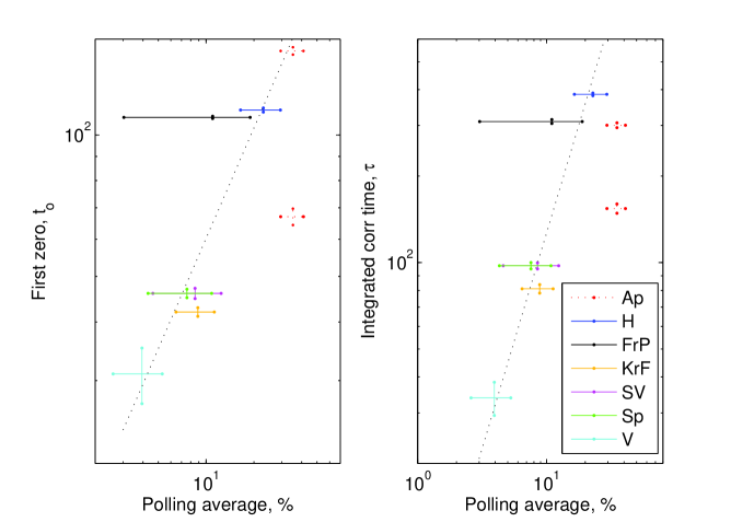
Figure 3: First anti-correlation time, $t_{0}$, and integrated correlation time, $\tau$, vs. polling average, $\overline{X}_{t}$, for the investigated parties. The data is plotted in a log-log plot and fitted with a best fit power-law functions $\tau\propto\overline{X}_{t}^{\beta_{t_{o}}}$ and $t_{0}\propto\overline{X}_{t}^{\beta_{\tau}}$. For the first zero-crossing time $\beta_{t_{0}}=0.78$ and for the integrated correlation time $\beta_{\tau}=1.50$

4.2 AWC analysis

In the left panel of figure 4 we have plotted the AWC results, scaled by $a^{-1/2}$ where $a$ is the time scale, as a function of the time scale for each political party. The error bars plotted in Figure 4 indicate $\pm$ one standard deviation for the wavelet coefficient based on 1000 samples where each sample have been added flat noise in the same fashion as in the calculation of the error bars for $\tau$ and $t_{0}$ above.

$\begin{array}[]{cc}\leavevmode\resizebox{195.12767pt}{}{\includegraphics[angle={0}]{fig4a}}&\leavevmode\resizebox{195.12767pt}{}{\includegraphics[angle={0}]{fig4b}}\end{array}$

Figure 4: Left: The average wavelet-coefficients on a given time scale, $a$, scaled with $a^{-1/2}$ as a function of the time scale. Right: The average wavelet-coefficients grouped into large and small political parties. The results are averages for all the parties in each group.

Looking at the polling average for all the parties (left panel of Figure 4), we can separate them into two groups. One group of large parties (Ap, H and FrP), and one group of small parties (SV, Sp, KrF and V). From Table 1 one can see that all parties within the same group have similar polling averages $\overline{X}_{t}$. They also have first crossing times $t_{0}$ in the same range. As a result we have averaged the AWC results for all the parties within each of the two groups, and the results can be seen in the right panel of Figure 4. The best linear fit on log-log scale is also inserted in the left panel of Figure 4. The averaged results suggest that the large parties have a Hurst exponent of 0.33 over the entire range that can be analysed by our sparse data, thus indicating anti-persistent behaviour in voter preferences for these parties. Since the larger parties are more likely to win the elections and form a Government, the anti-correlated behaviour seems to support the view that it is hard to remain in power for successive terms. Furthermore, the other parties will most certainly target voters from the leading party’s base hoping to win their preference, and this competition may contribute for the anti-persistence seen in the polling data for large parties. As we will see below, smaller parties are less susceptible to this effect.

As seen in both panels of Figure 4, the averaged wavelet coefficients for smaller parties show a shift in behaviour at about 1 to 3 years, or about 10 to 40 months. They cross over from a Hurst exponent close to zero for small time scales, indicating a highly anti-persistent trend, to a Hurst exponent of 0.67 for larger time scales indicating a correlated behaviour. The scale at which the crossover occurs is in the same range as the correlation measure $t_{0}$ for the smaller parties. For the larger parties $t_{0}$ is so large that we can not see any crossover in the wavelet analysis. This may indicate that the “recollection time” or memory in the smaller parties is of the order of 2 years, whereas for the larger parties it is considerably longer and possibly on the scale of decades.

5 Summary and Conclusions

In this paper we have put forward two different methods for measuring political memory, namely, correlation analysis and scaling analysis. To illustrate these measures, we have carried out an empirical analysis of monthly polling data for the major political parties of Norway over the last 30 years. It has been found that the integrated correlation time $\tau$ and the time of first occurrence of anti-correlation $t_{0}$ grow as a function of party size $\overline{X}_{t}$, and both have been found to display a power-law dependence: $\tau\propto\overline{X}_{t}^{1.50}$ and $t_{0}\propto\overline{X}_{t}^{0.78}$.

The polling records for all the parties show self-affine properties, and the Hurst exponent $H$ have been calculated using the AWC method. It has been shown that the polling records show anti-correlated behaviour with $H=0.33$ for large parties. For smaller parties a crossover from a highly anti-persistent trend $H=0.01$ to a correlated behaviour with $H=0.67$ has been found.

Taken in conjunction, the results from the correlation and scaling analyses show that the voter bases for the large parties have inherently long memories and this seems to lead to an mean-reverting trend in their electoral preferences. On the other hand, the smaller parties have little short-term memory and a highly anti-persistent behaviour at the small time scales, however for longer times they show a crossover to a persistent trend when the data sets become anti-correlated. Unfortunately, the time series are too short to show any crossover for larger parties.

The discussion above indicates that smaller parties, which are often perceived to fight for special interests, have over long time scales more persistent voters than the larger parties do. They have more rapidly varying polling data on small time scales, but on the longer time scales their voters are more loyal. On the other hand the large parties, often perceived as mass parties that appeal to a large fraction of the population, have slower varying polling data on short time scales in comparison to small parties, but on longer time scales their voters are less loyal.

References

References

- [1] Weart S R 2000 Never at war (New Haven: Yale University Press).
- [2] Hegre H et al. 2001 American Political Science Review 95 33.
- [3] Halperin M H, Siegle J T and Weinstein M M 2004 The Democratic Advantage: How Democracies Promote prosperity an Peace (London: Routledge).
- [4] Costa Filho R N, Almeida M P, Andrade Jr J S, and Moreira J E 1999, Physica A 60 1067.
- [5] Costa Filho R N, Almeida M P, Moreira J E, and Andrade Jr J S 2003, Physica A 322 698.
- [6] Fortunato S and Castellano C 2007, Phys. Rev. Lett. 99 138701.
- [7] Travieso G and Costa L D 2006, Phys. Rev. E 74, 036112.
- [8] Moreira A A, Paula D R, Costa Filho R N, and Andrade J S 2006, Phys. Rev. E 73 065101.
- [9] Schneider J J and Hirtreiter C 2005, Int.Jour. Phys. C 16 1165.
- [10] http://www.stortinget.no, official web-site for ”Stortinget”.
- [11] http://www.ssb.no, Norwegian Statistical Bureau.
- [12] http://www.regjeringen.no, official web-site for the Council of State.
- [13] Walpole R E, Myers R H and Myers S L 1998, Probability and Statistics for Engineers and Scientists (New Jersey: Prentice Hall).
- [14] Hurst H E 1951 Trans. Am. Soc. Civil Eng. 116 770.
- [15] Simonsen I, Hansen A and Nes O M 1998 Phys. Rev. E 58 3.
- [16] Barabási A-L and Stanley H E 1995, Fractal Concepts in Surface Growth (Cambridge: Cambridge Uni. Press).