Quantum Hall system in Tao-Thouless limit

Abstract

We consider spin-polarized electrons in a single Landau level on a torus. The quantum Hall problem is mapped onto a one-dimensional lattice model with lattice constant $2\pi/L_{1}$, where $L_{1}$ is a circumference of the torus (in units of the magnetic length). In the Tao-Thouless limit, $L_{1}\rightarrow 0$, the interacting many-electron problem is exactly diagonalized at any rational filling factor $\nu=p/q\leq 1$. For odd $q$, the ground state has the same qualitative properties as a bulk ($L_{1}\rightarrow\infty$) quantum Hall hierarchy state and the lowest energy quasiparticle exitations have the same fractional charges as in the bulk. These states are the $L_{1}\rightarrow 0$ limits of the Laughlin/Jain wave functions for filling fractions where these exist. We argue that the exact solutions generically, for odd $q$, are continuously connected to the two-dimensional bulk quantum Hall hierarchy states, ie that there is no phase transition as $L_{1}\rightarrow\infty$ for filling factors where such states can be observed. For even denominator fractions, a phase transition occurs as $L_{1}$ increases. For $\nu=1/2$ this leads to the system being mapped onto a Luttinger liquid of neutral particles at small but finite $L_{1}$, this then develops continuously into the composite fermion wave function that is believed to describe the bulk $\nu=1/2$ system. The analysis generalizes to non-abelian quantum Hall states.

I Introduction

The two-dimensional electron gas in a perpendicular magnetic field, the quantum Hall (QH) system, is remarkably rich. The integer QH effect shows a conductance precisely quantized in integer units of $e^{2}/h$ vonk , and in the fractional QH regime the conductance is quantized in fractions of $e^{2}/h$ and there are fractionally charged quasiparticles that obey (abelian) fractional statistics tsui ; stat1 ; stat2 . Whereas the integer effect can be understood in terms of non-interacting electrons it1 ; it2 , the fractional effect is caused by the interaction between the electrons Laughlin83 . Other states observed in this strongly correlated electron system are metallic states that resemble a free two-dimensional Fermi gas jiang ; willett90 ; wang and inhomogenous striped states in higher Landau levels striped1 ; striped2 . A further example of an exotic quantum state that may form is a non-abelian state where the quasiparticles obey non-abelian fractional statistics mr ; nayak ; readrezayi .

The fractional QH effect is understood as an incompressible quantum liquid with fractionally charged quasiparticles; this is based on Laughlin’s wave functions for filling fractions $\nu=1/(2m+1)$ Laughlin83 . For other fractions, a hierarchy construction where quasiparticles condense to form new quantum liquids just as electrons form the Laughlin states was proposed by Haldane hierarchyHaldane , Laughlin hierarchyLaughlin and by Halperin hierarchyHalperin . An alternative view, where electrons supposedly capture magnetic flux to form composite fermions that see a reduced magnetic field was developed by Jain jain89 ; jainrev1 ; jainrev2 ; jainbook . Successful mean field theories that support this idea of flux attachment have been developed zhang ; read89 ; lopez . The composite fermion approach has received strong support by experiments performed in the half-filled Landau level. Near $\nu=1/2$, ballistic transport is consistent with particles moving in a reduced magnetic field in accordance with the composite fermion prediction ballistic1 ; ballistic2 ; ballistic3 . At $\nu=1/2$, the external magnetic field is completely absorbed by the electrons and the composite fermions see no magnetic field—they form a two-dimensional Fermi gas. The mean field theory of this state hlr ; kalmeyer is in excellent agreement with surface acoustic wave experiments willett90 ; Willettreview .

In spite of these impressive results it is our opinion that there are basic questions concerning the QH system that remain to be answered. Most importantly, a microscopic understanding is lacking. It is true that good many-body wave functions exist, but there is no microscopic understanding or derivation of them. For example, according to the composite fermion picture the fractional QH ground state is formed when composite fermions fill an integer number of effective Landau levels in the reduced magnetic field. No derivation of this scenario from the many body wave function exists. Mean field theory, which is successful, does give support to the idea of electrons binding flux quanta; however, it is not understood why mean field theory works as well as it does. A further question is the relation between the original hierarchy description and composite fermions; are they alternative descriptions of the same thing as argued by Read read90 and by Blok and Wen blokwen , or are they fundamentally different as argued by Jain jain89 ; jainrev1 ; jainrev2 ; jainbook ? Our aim is to contribute to a solution to these problems.

In this article we consider spin-polarized interacting electrons within a single Landau level. It has recently been realized that there is a limit in which this problem can be exactly solved for any rational filling factor $\nu=p/q\leq 1$—and that the solution is physically relevant bk1 ; bk2 ; we06 ; hierarchy ; conformal . We here expand on, and provide details of, our work presented in Refs. bk1, ; bk2, . We consider the interacting electron gas on a torus where it becomes equivalent to a one-dimensional lattice model with a complicated long-range interaction. The solvable limit is the thin torus: $L_{1}\rightarrow 0$, where $L_{1}$ is one of the circumferences of the torus (the other circumference being infinite). In this limit the interaction in the one-dimensional lattice problem becomes purely electrostatic and the ground state is a ”crystal” of electrons occupying fixed positions on the lattice as far apart from each other as possible. For $\nu=1/3$ every third site is occupied; interestingly enough this is the state introduced by Tao and Thouless in 1983 to explain the fractional QH effect Tao83 and we call these crystal states Tao-Thouless (TT) states. The fractionally charged quasiparticles are domain walls separating the degenerate ground states that exist on the torus.

It should be noted that the mapping of the lowest Landau level, or of any single Landau level for that matter, onto a one dimensional lattice problem is exact and that varying $L_{1}$ may alternatively be thought of as varying a parameter in the hamiltonian that controls the range of the interaction while keeping the two-dimensional space fixed (and possibly infinite). To stress this we refer to the thin limit as the Tao-Thouless (TT) limit. If the ground state in the TT-limit remains the ground state as $L_{1}\rightarrow\infty$ we may thus conclude that the experimentally accessible ground state is adiabatically connected to the ground state in the TT-limit.

The simple limit $L_{1}\rightarrow 0$ may at first seem to be of little physical interest—it is really an extreme case: the interaction is both very short range and anisotropic and is furthermore purely electrostatic. The surprising fact is that the ground state in this limit has all the qualitative properties of a fractional quantum Hall state, such as a gap, the correct quantum numbers and quasiparticles with the correct fractional charge. We argue that the simple TT-ground states obtained in the TT-limit develop continuously, without a phase transition, into the fractional QH hierarchy states, as $L_{1}\rightarrow\infty$, for filling factors where such states are observed. Thus, we argue that the TT-state in general describes the fractional QH phase observed as $L_{1}\rightarrow\infty$, in the sense that these states are adiabatically connected. We show that the TT-states are the $L_{1}\rightarrow 0$ limits of the Laughlin and Jain wave functions for filling fractions where these exist. In the TT-limit the original hierarchy construction is manifest: the TT-ground states are condensates of quasiparticles.

The hierarchy structure of states in the TT-limit has recently emerged within a conformal field theory (CFT) construction of bulk hierarchy wave functions for all fractions that are obtained by successive condensation of quasielectrons (as opposed to quasiholes) hierarchy ; conformal . These wave functions reduce to the correct TT-states in the TT-limit and are obtained by a natural generalization of the conformal construction of the composite fermion wave functions hans . This supports the adiabatic continuity fro m the TT-limit to the bulk for general hierarchy states.

The TT-states are the ground states also for the even denominator fractions in the TT-limit; however, for these fractions we claim that there is always a phase transition when $L_{1}$ increases. This is supported by numerical studies and by a detailed analysis of $\nu=1/2$, which we believe is a representative case for the even denominator fractions.

At $\nu=1/2$, there is a phase transition from the gapped TT-state to a one-dimensional gapless state at $L_{1}\sim 5$. (Lengths are measured in units of the magnetic length, $\ell=\sqrt{\hbar c/eB}=1$.) Also for this gapless phase there is an exact solution: For a hamiltonian that is a good approximation at $L_{1}\sim 5$, the low energy sector consists of non-interacting neutral fermions (dipoles); the ground state is a one-dimensional Fermi sea and there are gapless neutral excitations. This provides an explicit example of interacting electrons in a magnetic field being equivalent to free particles that do not couple to the magnetic field. The ground state in the exact solution is a version of the composite fermion state jainbook given by Rezayi and Read rr . There is strong numerical evidence bk2 that this gapless one-dimensional state develops continuously, without a phase transition, into the two-dimensional bulk version of the Rezayi-Read state that is believed to describe the observed metallic state at $\nu=1/2$.

The Moore-Read pfaffian state mr , believed to describe the half-filled second Landau level, $\nu=5/2$, also exists in the TT-limit. A simple construction gives the quarter-charged quasiholes and quasielectrons as domain walls between the six-fold degenerate ground states and the non-trivial degeneracies for these excitations is obtained haldaneAPS ; we06 . Similar results for other non-abelian states exist seidel06 ; read06 ; weunpublished ; see also Ref. haldanejack, .

Over the years there have been many interesting attempts to improve the understanding of the QH system and it is impossible to here mention them all. In our work what emerges is a one-dimensional theory of the quantum Hall system which depends on a dimensionless parameter $L_{1}$, where the Tao-Thouless states Tao83 are the exact solutions as $L_{1}\rightarrow 0$ and the fractionally charged quasiparticles are domain walls between the degenerate ground states. The TT-states are adiabatically connected to bulk QH states as $L_{1}\rightarrow\infty$—there is no phase transition if a QH state is observed. Searching the literature one finds hints and suggestions for such a scenario. Anderson noted in 1983 that Laughlin’s wave function has a broken discrete symmetry and that the quasiparticles are domain walls between the degenerate ground states anderson . Furthermore he noted that the TT-state is non-orthogonal to the Laughlin state and suggested that it can be thought of as a parent state that develops into the Laughlin wave function, without a phase transition, as the electron-electron interaction is turned on. In 1984, Su concluded, based on exact diagonalization of small systems on the torus, that the QH state at $\nu=p/q$ is $q$-fold degenerate and that the lowest energy excitations are quasiparticles with charge $\pm e/q$ that are domain walls between the degenerate ground states su1984 ; su2 . In 1994, Rezayi and Haldane studied the Laughlin wave function on a cylinder as a function of its radius and noted that it approaches the Tao-Thouless state on the thin cylinder. Implicit in their work is the fact that the Laughlin wave function is the exact and unique ground state to a short range pseudo-potential interaction on a cylinder for any circumference Haldane94 . In retrospect, this makes a very strong case for an adiabatic evolution from the TT-state to the Laughlin wave function. A one-dimensional approach to QH states was also considered by Chui in 1985 chui1985 ; chui86 . More recently, this has been explored in connection with Bose-Hubbard models by Heiselberg heiselberg , and it should also be mentioned that Dyakonov presents a one-dimensional toy QH-model Dyakonov .

At $\nu=1/2$, we find that the low energy sector consists of weakly interacting dipoles. This relates to earlier descriptions in terms of dipoles, in particular to the field theory of Murthy and Shankar ms and the work by Read readearly ; read.5 , Pasquier and Haldane pasq , Lee dhlee and Stern et al stern ; for reviews see Ref. rev1, . It is of course also reminiscent of composite fermions in general jainbook in that the particles do not couple to the magnetic field and are weakly interacting.

We would also like to draw the attention to the construction of composite fermion wave functions directly in the lowest Landau level by Ginocchio and Haxton haxton , the series of work by Wojs, Quinn and collaborators, see Ref. wojs, and references therein. Explicit wave functions have been obtained within the original hierarchy construction by Greiter greiter94 .

The content of the article is as follows. The one-dimensional lattice model for interacting electrons in a single Landau level is introduced in Sec. II. In Sec. III we solve this problem exactly in the TT-limit $L_{1}\rightarrow 0$, ie we diagonalize the interacting electron hamiltonian for any rational filling factor in this limit. The ground states and the fractionally charged quasiparticles are identified and it is found that the former are condensates of the latter thus proving the original hierarchy construction in this limit hierarchy . The quasiparticles are domain walls between the degenerate ground states and their charge is determined by the Su-Schrieffer counting argument. The energy of a quasielectron-quasihole pair is determined as $L_{1}\rightarrow 0$ and it is found that the gap to creating an infinitely separated such pair at $\nu=p/q$ decreases monotonously with increasing $q$ but is independent of $p$; this is in surprisingly good agreement with experiments, which are performed in the two-dimensional bulk system, $L_{1}\rightarrow\infty$. The Laughlin and Jain fractions, as well as those observed by Pan et al pan are considered explicitly as examples, and finally the relation to composite fermions and emergent Landau levels is commented on.

The transition to the two-dimensional bulk system as $L_{1}\rightarrow\infty$ is considered in Sec. IV, first for odd denominator fractions leading to the QH hierarchy states, then for the half-filled Landau level; comments on other even denominator fractions and on non-abelian states are included. The conclusion is that the rich structure and different phases of matter present in the QH system exist also in the TT-limit, where it can be studied in detail starting from a microscopic hamiltonian.

Technical details are burried in a series of appendices. The mathematics that we need for a single Landau level on a torus Haldane85PRL including the construction of the lattice hamiltonian is given in Appendix A. In Appendix B we prove that the relaxation procedure given in Sec. III actually gives the ground state. In Appendix C, we show that the quasiparticle charge at $\nu=p/q$ is $e^{*}=\pm e/q$; the result is obtained in the limit $L_{1}\rightarrow 0$ using the Su-Schireffer counting argument. The energy of a quasielectron-quasihole pair is obtained in Appendix D. In Appendix E we show that the $L_{1}\rightarrow 0$ limit of Laughlin’s and Jain’s wave functions are the TT-ground states obtained in Sec. III. Appendix F shows that Laughlin’s wave function at $\nu=1/(2m+1)$ is the exact ground state, and that there is a gap to excitations, for all $L_{1}$ for a short-range interaction. Appendix G contains details of the exact solution at $\nu=1/2$.

II Model

We consider a single Landau level of spin-polarized electrons on a torus with lengths $L_{1},L_{2}$ in the $x$ and $y$-directions respectively. We use units such that $\hbar=c/eB=1$ and choose one-particle states $\psi_{k}$, $k=0,1,\dots,N_{s}-1$, $N_{s}=L_{1}L_{2}/2\pi$, that have $x$-momentum $2\pi k/L_{1}$ and are gaussians centered at $y=-2\pi k/L_{1}$, see Appendix A. This provides an exact mapping of the Landau level onto a one-dimensional lattice model with lattice constant $2\pi/L_{1}$, see Fig. 1. Each site can be either empty, 0, or occupied by an electron, 1. Thus a basis of many particle states is provided by $\{|n_{0}n_{1}n_{2}\dots n_{N_{s}-1}\rangle\}$, where $n_{i}=0,1$; alternatively, states can be characterized by the positions (or, equivalently, the $x$-momenta) $\{k_{1},k_{2},...,k_{N_{e}}\}$ of the particles.

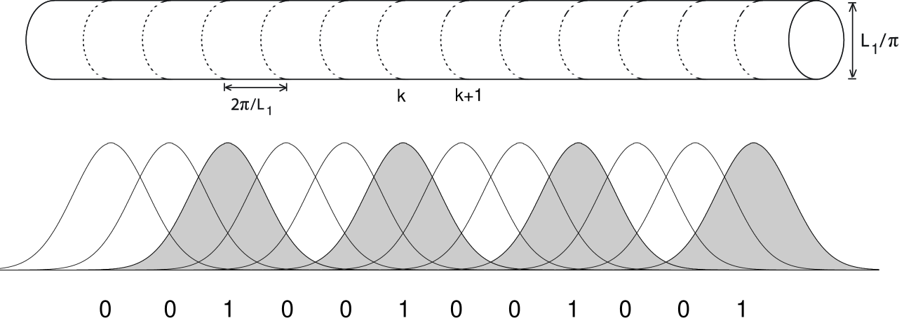
Figure 1: Mapping of a single Landau level onto a one-dimensional lattice model. The two-dimensional space is a cylinder with circumference $L_{1}$ (or a torus if the ends are identified) (top panel). The single particle wave functions are centered along circles and are gaussians of width one along the cylinder (central panel); they are numbered by their momenta $k2\pi/L_{1}$ which also give the position along the cylinder. This gives a one-dimensional lattice model with lattice constant $2\pi/L_{1}$ where each site is either empty (0) or occupied by en electron (1). As an example the Tao-Thouless state 001 at $\nu=1/3$ is shown (bottom panel).

A general two-body interaction, $V(r)$, that depends on the distance, $r$, between two electrons only, such as a Coulomb or a short-range delta function interaction, leads to the one-dimensional hamiltonian

$$\mbox{$$}H = \!\!\sum_{n=0}^{N_{s}-1}\sum_{|m|<k\leq N_{s}/2}\frac{V_{km}}{\!1\!+\!\delta_{k,\frac{N_{s}}{2}}\!\!}c^{\dagger}_{n+m}c^{\dagger}_{n+k}c_{n+k+m}c_{n}\ .$$ (1)

Here $c^{\dagger}_{k}$ creates an electron in state $\psi_{k}$, $\{c_{k},c_{m}^{\dagger}\}=\delta_{km}$, and $V_{km}=V_{k,-m}$. $H$ consists of the two-body terms that preserve the $x$-momentum, ie, the position of the center of mass of the electron pair, see Fig. 2. $V_{km}$ is the amplitude for two electrons separated $k-m$ lattice constants to hop symmetrically to a separation of $k+m$ lattice constants. $V_{k0}$ is the electrostatic repulsion (including the exchange interaction) between two electrons separated $k$ lattice constants.

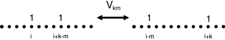
Figure 2: A general translationally invariant two-electron interaction consists of the terms where two electrons preserve the position of their center of mass. There are electrostatic terms $V_{k0}$, where the electrons do not move, and hopping terms $V_{km},\,m\neq 0$, where the electrons hop symmetrically.

For a given real-space interaction $V(r)$, when $L_{1}$ is small the lattice constant $2\pi/L_{1}$ is large and, hence, the dominant $V_{km}$ are those with small $k,m$. Furthermore, the wave functions $\psi_{k}$ are gaussians in the $y$-direction, with width of the order of the magnetic length, hence their overlap vanishes rapidly as $L_{1}\rightarrow 0$, and the electrostatic terms $V_{k0}$ dominate in this limit. The physics is thus very simple in the TT-limit $L_{1}\rightarrow 0$—it is determined by electrostatic repulsion only. In the two-dimensional limit, $L_{1}\rightarrow\infty$, the range of the one-dimensional interaction measured in number of lattice constants goes to infinity for any real space two-dimensional interaction; this is true also for a local interaction such as $V(r)\propto\bigtriangledown^{2n}\delta^{2}({\bf r})$.

The symmetry analysis of many-electron states on the torus was given by Haldane Haldane85PRL ; a simple version adapted to our needs can be found in Appendix A. We give here the results. There are two translation operators, $T_{\alpha}$, $\alpha=1,2$, that commute with the hamiltonian $H$; they obey $T_{1}T_{2}=e^{2\pi ip/q}T_{2}T_{1}$, see (38). These operators have eigenvalues $e^{2\pi iK_{\alpha}/N_{s}},K_{\alpha}=0,...,N_{s}-1$. $T_{1}$ corresponds to $x$-translations and $K_{1}=\sum_{i=1}^{N_{e}}k_{i}$ is the total $x$-momentum (in units of $2\pi/L_{1}$). $T_{2}$ translates the system one lattice constant in the $y$-direction, ie along the one-dimensional lattice and increases $K_{1}$ by $N_{e}$. At filling factor $\nu=p/q$ (where $p$ and $q$ are relatively prime) $T_{2}^{q}$ commutes with $T_{1}$: $\{H,T_{1},T_{2}^{q}\}$ is a maximal set of commuting operators. $T_{2}^{k},k=0,1,\dots q-1$, generate $q$ degenerate orthogonal states, which have different $K_{1}$, when acting on any state—this is the $q$-fold center of mass degeneracy. Hence, each energy eigenstate is (at least) $q$-fold degenerate and we choose to characterize it by the smallest $K_{1}$. Thus, the energy eigenstates are characterized by a two-dimensional vector $K_{\alpha}=0,...,N_{s}/q-1$, where $e^{2\pi iK_{2}q/N_{s}}$ is the $T_{2}^{q}$-eigenvalue.

III Exact solution

In this section we solve the problem of interacting spin-polarized electrons exactly at any rational filling factor $\nu=p/q\leq 1$ in the Tao-Thouless limit; we diagonalize the hamiltonian (1) and construct explicitly the ground state as well as the low energy charged excitations which turn out to have charge $\pm e/q$. As noted above, the hopping elements, $V_{km},\,m\neq 0$, vanish rapidly as $L_{1}$ decreases, whereas the electrostatic elements, $V_{k0}$, decrease much more slowly. Hence in the limit $L_{1}\rightarrow 0$ effectively only the electrostatic interaction survives and the hamiltonian (1) becomes

$$\mbox{$$}H_{0}=\sum_{i=0}^{N_{s}-1}\sum_{1\leq k\leq N_{s}/2}\!\frac{V_{k0}}{\!1\!+\!\delta_{k,\frac{N_{s}}{2}}\!\!}\ \hat{n}_{i}\hat{n}_{i+k}\ \ ,$$ (2)

where $\hat{n}_{i}=\hat{c}_{i}^{\dagger}\hat{c}_{i}$ and periodic boundary conditions have been imposed, $\hat{n}_{i+N_{s}}=\hat{n}_{i}$. $H_{0}$ in (2) defines the Tao-Thouless limit. At filling fraction $\nu=p/q=N_{e}/N_{s}$, the energy eigenstates are simply the states

$$\mbox{$$}\{|n_{0}n_{1}\dots n_{N_{s}-1}\rangle\}\ \ ,\ \ \ n_{i}=0,1\ \ ,$$ (3)

where $N_{e}$ electrons occupy fixed positions on $N_{s}$ lattice sites,

$$\mbox{$$}\sum_{i=0}^{N_{s}-1}n_{i}=N_{e}=N_{s}p/q\ \ .$$ (4)

III.1 Ground states, quasiparticles and the hierarchy

Here we determine the ground state at $\nu=p/q\leq 1$ in the TT-limit, ie for the hamiltonian $H_{0}$ in (2). This is the classical electrostatics problem of finding the position of $N_{e}$ electrons, on a circle with $N_{s}$ sites, that minimizes the energy. Hubbard gave an algorithm for constructing this ground state hubbard ; we will present two simple alternative constructions. The first gives the ground state for given $\nu=p/q$, and provides an intuitive understanding of why the energy is minimized; the second starts from $\nu=1/q$ and constructs the ground states at all other filling factors iteratively from this state as repeated condensations of quasiparticles—in addition to the ground states this gives the fractionally charged quasiparticles and makes the Haldane-Halperin hierarchy construction manifest in the TT-limit.

The states obtained here are the ground states for any interaction that obeys the concavity condition

$$V_{k+1,0}+V_{k-1,0}>2V_{k0}\ \ \ ,$$ (5)

which implies, by iteration,

$$\mbox{$$}V_{k+n,0}+V_{k-1,0}>V_{k+n-1,0}+V_{k0}\ \ ,$$ (6)

for all $k,n>0,\ k+n<N_{s}$. When, $L_{1}\rightarrow 0$, $V_{k0}$ is simply the electrostatic interaction energy between two rings of circumference $L_{1}$ separated a distance $k2\pi/L_{1}$; hence he concavity condition is fulfilled by a generic electron-electron interaction when $L_{1}\rightarrow 0$. It implies that the interaction energy of one electron with two other electrons that have fixed positions is minimized if the first electron is as close to the midpoint between the fixed electrons as possible, ie if the distances to the two fixed electrons differ by at most one lattice constant, see Fig. 3.

The crucial observation in obtaining the ground state is to realize that it is possible to minimize the energies of the $k$:th nearest neighbors separately for each $k$ for an interaction that obeys (6) hubbard .

Figure 3: The interaction energy of one movable electron with two fixed electrons is minimized when the distances to the two fixed electrons differ by at most one lattice site.

In our first construction, the ground state is obtained by placing the electrons equidistantly on a circle and then letting them relax to the closest lattice sites. The ground state is periodic with a unit cell of length $q$ containing $p$ electrons and this cell is obtained as follows. Consider a circle with $p$ equidistant electrons and a lattice with $q$ (equidistant) lattice sites as in Fig. 4. Move each electron to its closest lattice site; an electron that is equally far from two sites is moved to one of these sites. The obtained configuration is the unit cell of the ground state, for the proof we refer to Appendix B. An algebraic expression for the unit cell is obtained by noting that electron $\alpha$ is at site

$$\mbox{$$}i(\alpha)=I[\alpha/\nu]\ \ \ ,$$ (7)

where $\alpha=0,\dots,p-1$ and $I[x]$ denotes the integer closest to $x$. For example, for $\nu=5/13$, (7) gives $\{I[\alpha/\nu]\}=\{0,3,5,8,10,(13,\ldots)\}$ and hence the unit cell is $1001010010100\simeq(0_{2}101)_{2}0_{2}1$ in agreement with Fig. 4. We use a chemical notation where the subscript denotes the number of times the quantity is repeated. That the unit cell at $\nu=p/q$ has length $q$ implies that the ground state is $q$-fold degenerate. This is the center of mass degeneracy of any state at $\nu=p/q$ discussed in Sec. II Haldane85PRL . For the quantum Hall states this is the topological degeneracy of the ground state identified by Wen and Niu wen ; wenreview .

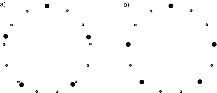
Figure 4: Ground state unit cell at $\nu=5/13$ by relaxation on circle. a) p=5 equidistant electrons on a circle with q=13 lattice sites; b) each electrons moved to its closest site, unit cell is $(0_{2}101)_{2}0_{2}1$.

Incidentally, the initial configuration with equidistant electrons is clearly the ground state in the continuum problem when there is no lattice—when there is a lattice the ground state is as similar to the continuum one as possible. Because of the periodicity, the picture of course generalizes immediately to the full system consisting of $N$ unit cells and periodic boundary conditions: the ground state for $N_{e}$ electrons on $N_{s}$ sites is obtained by starting with equidistant electrons and moving each electron to its closest site.

At $\nu=1/q$ the procedure gives the unit cell $0_{q-1}1$. Thus, the ground state is obtained by placing one electron on every $q$:th site; this obviously minimizes the electrostatic repulsion. For odd $q$, these are the Laughlin fractions and the state with unit cell $0_{q-1}1$ was in fact proposed by Tao and Thouless in 1983 as an explanation of the fractional quantum Hall effect Tao83 . Although this state has a small overlap with the exact ground state (for large $L_{1}$), and with the Laughlin state, it does in fact play an important role in the quantum Hall effect and we will call the crystal ground states at general $\nu=p/q$ Tao-Thouless (TT) states. We claim that the TT-states are QH-states in the sense that they are adiabatically connected to the bulk QH states bk2 ; hierarchy .

Note that the TT-states have a gap to excitations—the lattice sites are fixed in space and there are no phonons in these crystals; the TT-states should not be confused with Wigner crystals, which have gapless excitations due to the broken translational invariance. This is a further reason to call the states considered here TT-states rather than crystal states.

We will now present an alternative, iterative, construction of the TT-states that brings out the connection to the hierarchy of fractional quantum Hall states hierarchyHaldane ; hierarchyHalperin and determines the fractionally charged quasiparticles. Let ${\bf C}^{(n)},n=0,1,2,\dots$ be the unit cell for a TT-state at level $n$; this level is defined by the iteration process and is identical to the one in the hierarchy construction. At the first levels we have

$${\bf C}^{(0)} = 0\ \ ,\ \ \ \nu_{0}=0$$

$${\bf C}^{(1)} = 0_{t_{1}-1}1\ \ ,\ \ \ \nu_{1}=\frac{1}{t_{1}}\ \ ,$$ (8)

where $t_{1}=1,2,\dots$. The unit cells for the TT-states at level $n\geq 2$ are obtained iteratively as

$$\mbox{$$}{\bf C}^{(n)} = {\bf C}^{(n-1)}_{t_{n}}{\bf C}^{(n-2)},\ \ \ \nu_{n}=\frac{t_{n}p_{n-1}+p_{n-2}}{t_{n}q_{n-1}+q_{n-2}}\ \$$

$${\bf C}^{(n)} = {\bf C}^{(n-1)}_{t_{n}-1}\overline{{\bf C}^{(n-2)}},\ \ \ \nu_{n}=\frac{t_{n}p_{n-1}-p_{n-2}}{t_{n}q_{n-1}-q_{n-2}}\ \ ,$$ (9)

where ${\bf C}^{(n-1)}_{t}$ indicates that ${\bf C}^{(n-1)}$ is repeated $t$ times; $\overline{{\bf C}^{(n-2)}}$ is the complement of ${\bf C}^{(n-2)}$ in the unit cell ${\bf C}^{(n-1)}$, ie ${\bf C}^{(n-2)}\overline{{\bf C}^{(n-2)}}={\bf C}^{(n-1)}$ and $\nu_{n}=p_{n}/q_{n}$. At the second level we obtain:

$$\mbox{$$}{\bf C}^{(2)} = \{0_{t_{1}-1}1\}_{t_{2}}{0}\ \ ,\ \ \ \nu_{2}=\frac{1}{t_{1}+\frac{1}{t_{2}}}$$

$${\bf C}^{(2)} = \{0_{t_{1}-1}1\}_{t_{2}-1}0_{t_{1}-2}1\ \ ,\ \ \ \nu_{2}=\frac{1}{t_{1}-\frac{1}{t_{2}}}\ \ .$$ (10)

We can now connect to the original hierarchy construction. As will be further discussed below, ${\bf C}^{(0)}=0$ is the quasihole, and $\overline{{\bf C}^{(0)}}=0_{t_{1}-2}1$ is the quasielectron, with charges $e^{*}=\pm e/t_{1}$, in the ground state ${\bf C}^{(1)}=0_{t_{1}-1}1$. Thus the unit cells ${\bf C}^{(2)}$ at level two consists of $t_{2}$ (or $t_{2}-1$) copies of the unit cell at level one, followed by a quasihole (or quasielectron) in the level one ground state—the new ground state at level two is a condensate of quasiparticles in the level one ground state.

At the next level, level three, we find the unit cells

$$\mbox{$$}{\bf C}^{(3)} = \{\{0_{t_{1}-1}1\}_{t_{2}}{0}\}_{t_{3}}0_{t_{1}-1}1$$

$${\bf C}^{(3)} = \{\{0_{t_{1}-1}1\}_{t_{2}}{0}\}_{t_{3}-1}\{0_{t_{1}-1}1\}_{t_{2}-1}0$$

$${\bf C}^{(3)} = \{\{0_{t_{1}-1}1\}_{t_{2}-1}0_{t_{1}-2}1\}_{t_{3}}0_{t_{1}-1}1\ \$$ (11)

$${\bf C}^{(3)} = \{\{0_{t_{1}-1}1\}_{t_{2}-1}0_{t_{1}-2}1\}_{t_{3}-1}\{0_{t_{1}-1}1\}_{t_{2}-2}0_{t_{1}-2}1$$

and the corresponding filling factors

$$\mbox{$$}\nu_{3} = \frac{1}{t_{1}+\frac{1}{t_{2}\pm\frac{1}{t_{3}}}}$$

$$\nu_{3} = \frac{1}{t_{1}-\frac{1}{t_{2}\pm\frac{1}{t_{3}}}}\ \ \ .$$ (12)

Generalizing this, we find at level $n$, the filling factors

$$\mbox{$$}\nu_{n}=\frac{1}{t_{1}+\frac{\alpha_{2}}{t_{2}+\frac{\alpha_{3}}{\frac{{\cdot_{\cdot}}}{t_{n-1}+\frac{\alpha_{n}}{t_{n}}}}}}\ \ \ ,$$ (13)

where $t_{i}=1,2,\dots$ and the corresponding unit cells are obtained using (III.1). In this construction, $\alpha_{i}=+1\,(-1)$ if ${\bf C}^{(i)}$ is constructed with ${\bf C}^{(i-2)}$ ($\overline{{\bf C}^{(i-2)}}$) in (III.1). A state at level $n$ is uniquely characterized by the parameters $\{t_{1},\alpha_{2}t_{2},\alpha_{3}t_{3},\dots,\alpha_{n}t_{n}\}$. Equation (13) is the continued fraction form of the filling factors as given by the hierarchy scheme, except that now also even denominators are obtained. Restricting to $t_{1}=1,3,5,\dots$ and $t_{i}=2,4,6,\dots$, for $i\geq 2$, (13) is identical to Haldane’s formula for the filling factors hierarchyHaldane , which is known to give each odd denominator fraction once.

This construction gives each rational filling factor $0\leq\nu\leq 1$ and by inspecting the unit cells one finds that they are such that the distances between $k$:th nearest neighbors differ by one lattice constant at most, hence they minimize the energy and are identical to the ground states obtained by the relaxation procedure above. To be precise, we have not proven that the unit cells obtained by the two methods are always identical, but we have checked this in many examples and are convinced that this is the case.

The interpretation of (III.1) as a condensate of quasiparticles generalizes to arbitrary level $n$ in (III.1):

$$\mbox{$$}{\bf C}^{(n-2)}\ \ {\rm and}\ \ \overline{{\bf C}^{(n-2)}}$$ (14)

are the quasihole and the quasielectron (which is which depends on the state) in the ground state with unit cell ${\bf C}^{(n-1)}$, and the ground state at level $n$, ${\bf C}^{(n)}$, is a condensate of these quasiparticles in accordance with the hierarchy construction. That the proposed quasiparticles, ${\bf C}^{(n-2)}$ and $\overline{{\bf C}^{(n-2)}}$, have the expected charges $e^{*}=\pm e/q$ at $\nu=p/q$ follows from the Su-Schrieffer counting argument Schrieffer , see Appendix C. Furthermore, they are domain walls between the degenerate TT ground states. This was noted by Anderson anderson and stressed by Su su1984 ; su2 based on exact diagonalization studies on the torus. The quasiparticles discussed here are the ones with the elementary charge $e^{*}=\pm e/q$ and the QH states are the simple abelian ones; as pointed out by Wen wenreview other quasiparticles may also in principle condense to form more complicated ground states.

The iteration formula (III.1) gives the one quasiparticle excitations in the state with unit cell ${\bf C}^{(n)}$ and shows that these are the lowest energy excitations at the corresponding filling factors; for example, inserting $01$ in the ground state with unit cell ${\bf C}^{(2)}=00101$ gives the quasielectron and it is the lowest energy state at $\nu=(2t_{2}+1)/(5t_{2}+2)$.

The energy of a quasielectron-quasihole pair at $\nu=p/q$ can be calculated in the limit $L_{1}\rightarrow 0$. According to the discussion above, the quasiparticles in a TT-state with unit cell ${\bf C}^{(n)}$ are ${\bf C}^{(n-1)}$ and $\overline{{\bf C}^{(n-1)}}$. Thus, a minimally separated particle-hole pair is obtained by the replacement

$$\mbox{$$}{\bf C}^{(n)}={\bf C}^{(n-1)}\overline{{\bf C}^{(n-1)}}\rightarrow\overline{{\bf C}^{(n-1)}}{\bf C}^{(n-1)}\ \ ,$$ (15)

in the ground state. Note that the replacement in (15) amounts to a translation of the unit cell ${\bf C}^{(n-1)}$ with periodic boundary conditions on the cell itself, thus it creates two domain walls (with the expected charge). It can be shown, see Appendix D, that $\overline{{\bf C}^{(n-1)}}{\bf C}^{(n-1)}$ differ from ${\bf C}^{(n)}$ only in that one electron has been moved one lattice constant.

A separated particle-hole pair is obtained by translating $s$ consecutive cells as in (15), ie with periodic boundary conditions on each cell separately, or, equivalently, on all $s$ of them together. This is equivalent to inserting a string of $s-1$ unit cells ${\bf C}^{(n)}$ between the particle and hole

$$\mbox{$$}{\bf C}^{(n)}_{s}\rightarrow\overline{{\bf C}^{(n-1)}}{\bf C}^{(n)}_{s-1}{\bf C}^{(n-1)},\$$ (16)

and moves $s$ electrons (one in each unit cell) one lattice constant in the same direction.

The replacement (15) or (16) implies an ordering of the particle-hole pair. The opposite ordering is obtained by instead making the reverse replacement

$$\mbox{$$}{\bf C}^{(n)}_{s}\rightarrow{\bf C}^{(n-1)}{\bf C}^{(n)}_{s-1}\overline{{\bf C}^{(n-1)}}\ \ .$$ (17)

Again the replacement (16) or (17) amounts to a translation of ${\bf C}^{(n)}_{s}$ assuming periodic boundary conditions.

It is shown in Appendix D that the energy of the separated particle-hole pair in (16,17) is

$$\mbox{$$}E_{\rm ph}(s)=\sum_{k=1}^{s-1}k\Delta_{kq}+s\sum_{s\leq k\leq N_{s}/2q}\frac{\Delta_{kq}}{1\!+\!\delta_{k,\frac{N_{s}}{2q}}\!\!}\ \ ,$$ (18)

where

$$\Delta_{kq}\equiv V_{kq-1,0}-2V_{kq,0}+V_{kq+1,0}\ \ .$$ (19)

$\Delta_{kq}$ is the change in energy for an electron with its two neighbors $k$ unit cells away when the initial electron is moved one lattice constant. This energy, which is the second derivative of $V_{k0}$, is positive due to the concavity condition (5), which thus ensures the stability of the TT-ground state to particle-hole formation. Note that $E_{\rm ph}(s)$ is independent of the numerator $p$ of the filling factor.

It can be shown that the nearest neighbor pair excitation $s=1$, which has energy

$$\mbox{$$}E_{\rm ph}(1)=\sum_{1\leq k\leq N_{s}/2q}\frac{\Delta_{kq}}{1\!+\!\delta_{k,\frac{N_{s}}{2q}}\!\!}\ \ ,$$ (20)

according to (18), is the lowest energy excitation at fixed filling fraction, see Appendix D.

An important quantity is the energy of an infinitely separated particle-hole pair; this is what is measured in activated transport and is a measure of the stability of a quantum Hall state. When the separation of the particles goes to infinity, $s\rightarrow\infty$, we find

$$E_{\rm gap}\equiv E_{\rm ph}(\infty)=\sum_{k=1}^{\infty}k\Delta_{kq}\ .$$ (21)

Note that the gap depends only on the denominator $q$, ie on the fractional charge $\pm e/q$, and not on the numerator $p$ in $\nu=p/q$.

This is natural in the sense that the denominator determines the charge of the quasiparticles, but the result is non-trivial since the properties of the ground states depend on both $p$ and $q$. Furthermore, $E_{\rm gap}$ is a monotonic function that approaches zero from above as the denominator $q$ increases. In this context it should be mentioned that Halperin within the original hierarchy construction of fractional QH states predicted a gap that is predominantly determined by $q$ and decreases monotonously with increasing $q$ hierarchyHalperin .

Thus we find that the gap to creating a separated quasiparticle pair decreases monotonously with increasing $q$. This motivates Fig. 5 which shows $1/q$ for each $\nu=p/q$, $q$ odd hierarchy . Each point corresponds to a TT-state that we claim is adiabatically connected to a bulk QH-state. The higher up a point is, the larger is the gap in the corresponding TT/QH-state and the more stable is the state. The points marked by plusses are filling fractions where a dip in the longitudinal resistance $R_{xx}$ is reported in the experiment by Pan et al pan . At the crosses, we infer a very small dip in the same data. This experiment, which covers the range $2/7\leq\nu\leq 2/3$ marked in the figure, is performed on the highest available mobility samples and exhibits the largest number of QH states. We note that to a surprisingly good approximation a dip in $R_{xx}$ is observed at a filling factor $\nu=p/q$ if, and only if, $q\leq q_{0}\approx 17$. This is in agreement with the gap, $E_{\rm gap}$, being independent of $p$.

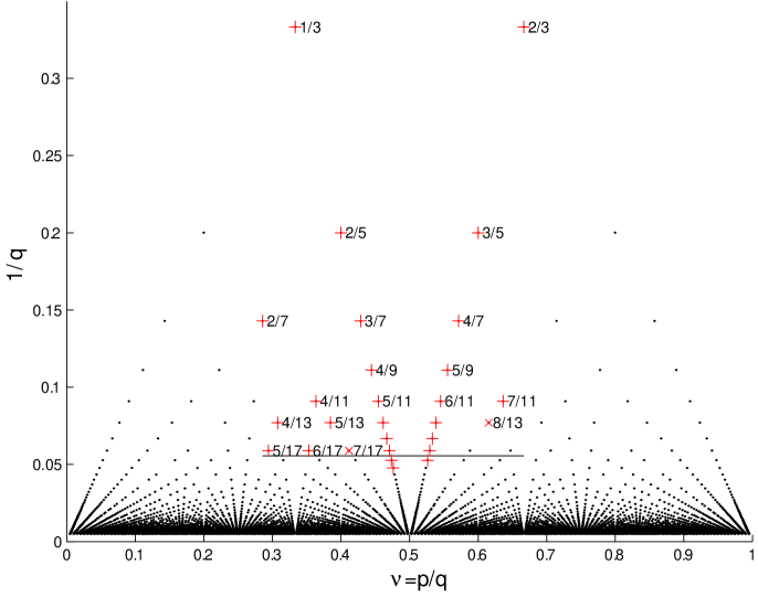
Figure 5: The Tao-Thouless states and their stability. Each point $(p/q,1/q)$, $q$ odd, corresponds to a TT-state that we claim is adiabatically connected to a bulk QH-state. The gap, and hence the stability, increases with decreasing $1/q$. At the points marked by plusses or crosses indications of QH-states are observed pan . The line is at constant gap and shows the range of the experiment in $\nu$. It is an approximate lower boundary in $1/q$ for the observed states.

The structure shown in Fig. 5 is a fractal, self-similar, one: enlarging any region of $\nu$ reproduces the original figure mani ; goerbig . This fractal structure is connected to the hierarchy construction of fractional QH states. The TT-states and their quasiparticles obtained when $L_{1}\rightarrow 0$ makes the hierarchy construction of fractional QH states manifest as discussed above. According to (III.1), for each state, the parent state, condensation of quasiparticles gives rise to two sequences of daughter states with filling fractions approaching that of the parent state from above and below respectively and with decreasing $1/q$, see Fig. 6. This holds for each $\nu=p/q$ and explains the fractal structure in Fig. 5. For a more complete discussion of the connection to the hierarchy theory, including the connection to the global phase diagram global ; lutken , we refer to Ref. hierarchy, .

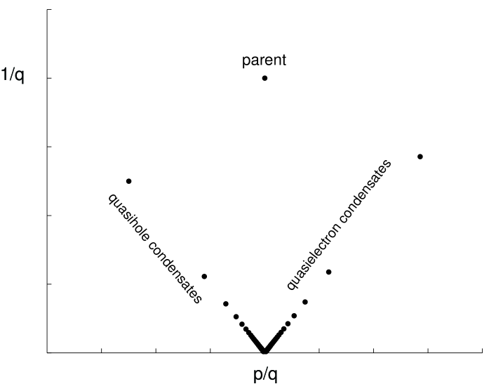
Figure 6: The hierarchy state at $\nu=p/q$ is the parent state for two sequences of daughter states formed by condensation of quasielectrons and quasiholes in the parent state.These sequences approach $p/q$, with decreasing gap $\sim 1/q$, from above and below respectively. Repeating this construction ad infinitum gives the fractal structure in Fig. 5.

Using Fig. 5 we can predict what QH-states are next in line to be discovered when higher mobility samples become available. For example, in the region $2/7\leq\nu\leq 2/3$ we first expect, in addition to 7/17 and 8/13 included above and new Jain states at $p/(2p\pm 1)$, states at 10/17, 11/17, 6/19, 7/19 and 8/19.

III.2 Examples

We here give explicit examples of TT ground states and quasiparticles for prominent filling fractions.

III.2.1 Laughlin/Jain fractions

For the Jain sequences $\nu=p/(2mp+1)$ that for fixed $m$ approach $\nu=1/2m$ from below as $p$ increases, the unit cell of the TT-state is $0_{2m}1(0_{2m-1}1)_{p-1}$; in the hierarchy notation this corresponds to $\{t_{1},\alpha_{2}t_{2},\dots,\alpha_{p}t_{p}\}=\{2m+1,-2,-2\dots,-2\}$. Thus the states in the Jain sequences are those in the hierarchy where all but the first condensate has maximal density. At $\nu=1/2m$, the unit cell is $0_{2m-1}1$. Explicitly for the experimentally most prominent sequence, $m=1$, the unit cells are

$$\mbox{$$}1/3 : \ 001$$

$$2/5 : \ 00101$$

$$3/7 : \ 0010101$$

$$4/9 : \ 001010101$$

$$5/11 : \ 00101010101$$

$$\dot{}$$

$$\dot{}$$

$$\dot{}$$

$$1/2 : \ 01\ \ \ .$$ (22)

By taking the particle-hole conjugate, $0\leftrightarrow 1$, of the states in (III.2.1) one obtains the Jain series $\nu=p/(2p-1)$ that approaches $1/2$ from above.

We now turn to the fractionally charged quasiparticles. Consider to start with the TT-state at $\nu=1/3$. According to (III.1), its unit cell is ${\bf C}^{(1)}=001$ and the quasiparticles are ${\bf C}^{(0)}=0$ and $\overline{{\bf C}^{(0)}}=01$. A quasihole with charge $e/3$ is created by inserting ${\bf C}^{(0)}=0$ somewhere:

$$001001001001001001001001001001001001001$$ (23)

$$00100100\underline{0}1001001001001001001001001001001$$

$$00100100\underline{0}100100100100\underline{0}100100100\underline{0}1001001\underline{001}\ .$$

The first line in (LABEL:qh1/3) is the ground state; the second line has one extra 0 inserted—comparing to the ground state it is clear that this creates a domain wall between two degenerate ground states. In the third line, three well-separated 0’s are inserted, creating three domain walls. Comparing to the ground state in the first line one sees that far away from the three 0’s the state is unchanged and to maintain the size of the system the underlined unit cell $001$ has to be removed. In between the inserted 0’s the state is a rigid translation of the original ground state and thus indistinguishable from this state by a measurement that only refers to the translated state. Thus, the net change is that one electron has been removed and this charge is divided on the three well-separated domain walls which thus have charge $e/3$ each. This is of course nothing but the Su-Schrieffer counting argument Schrieffer . The argument is also closely related to Laughlin’s original argument for the fractional charge, where a quasihole was created by adiabatic insertion of a flux quantum Laughlin83 —this corresponds to adding one empty site as there is one site per flux quantum.

The quasielectron is created by inserting $\overline{{\bf C}^{(0)}}=01$: 00100100101001001001001. Again this is a domain wall and the charge is, by the counting argument $-e/3$. Note that particle-hole symmetry is manifest; this is not the case for the bulk wave functions. It is straightforward to show that the excitations just given are the $L_{1}\rightarrow 0$ limits of the two-dimensional bulk quasiparticles constructed by Laughlin, see Appendix E.

It follows from Sec. III that inserting or removing 01 create quasiparticles in all the TT ground states in the Jain sequence $\nu=p/(2p\pm 1)$ that approaches $1/2$ as $p$ increases. For example, a quasielectron at $\nu=2/5$ is obtained as:

$$00101001010010100101001010010100101$$

$$0010100101\underline{01}0010100101001010010100101\ \ .$$ (24)

For Jain sequences with general $m$, starting from the Laughlin state $\nu=1/(2m+1)$, quasiholes (quasielectrons) are created by removing (inserting) $0_{2m-1}1$. In all cases, the Su-Schrieffer counting argument gives the expected charge, $\pm e/(2mp+1)$, for these quasiparticles and they are the $L_{1}\rightarrow 0$ limits of the Laughlin and Jain quasiparticles in the two-dimensional bulk system, see Appendix E.

III.2.2 Non-Jain fractions

Until recently, all experimentally well-established fractional quantum Hall states where for Laughlin-Jain filling fractions. However, in 2003 Pan et al reported a new set of states in ultra-high mobility samples pan . Preliminary indications of such a state at 4/11 was reported by Goldman and Shayegan goldman . Fractional quantum Hall states were seen at the following odd denominator filling factors $\nu=4/11,7/11,4/13,5/13,(8/13),5/17,6/17$ and $(7/17)$ (the ones in parenthesis are inferred by us from the data in Ref. pan, but were not claimed in this reference). Using the methods above, we readily find the TT ground states and the quasiparticles with charge $e^{*}=\pm e/q$ at these filling fractions. In Table 1 the unit cells are given in the hierarchy form, ie as in (III.1). The anti-quasiparticle, which is not given in the table, is obtained by taking the complement of the quasiparticle in the given ground state unit cell, according to (14). The unit cell for given $\nu=p/q$ is most easily obtained using the relaxation method, (7); it is then easily transformed to the hierarchy form by identifying its parent using Figs. 5 and 6. The parent is one of the two nearest neighbors whose denominator is smaller than $q$. —tt Check this

Table 1: Ground states and quasiparticles in the TT-limit for the odd denominator fractions observed by Pan et al pan that do not belong to the Jain sequence.

$\nu$	ground state	quasiparticle
4/11	$\{0_{2}1\}_{3}01$	$0_{2}1$
7/11	$\{1_{2}0\}_{3}10$	$1_{2}0$
4/13	$\{0_{2}1\}_{4}0$	$0_{2}1$
5/13	$\{0_{2}101\}_{2}0_{2}1$	$0_{2}101$
8/13	$\{1_{2}010\}_{2}1_{2}0$	$1_{2}010$
5/17	$\{\{0_{2}1\}_{2}0\}_{2}0_{2}1$	$\{0_{2}1\}_{2}0$
6/17	$\{0_{2}1\}_{5}01$	$0_{2}1$
7/17	$\{0_{2}101\}_{3}01$	$0_{2}101$

III.3 Emergent Landau levels and composite fermions

We have seen that in the TT-limit the TT ground states give a microscopic realization of the original hierarchy construction of fractional quantum Hall states. Today the alternative construction of quantum Hall states in terms of composite fermions has become the dominant framework and one may ask how the TT-construction is related to this. We believe, as argued by Read read90 and by Blok and Wen blokwen but contrary to the opinion of Jain jainrev1 ; jainrev2 ; jainbook , that the original hierarchy construction and composite fermions are just two different ways to view the same phenomena. In our approach, this is supported by the fact that both the hierarchy construction and the emergent Landau level structure is manifest in the TT-limit and that the TT-ground states and the quasiparticles are the $L_{1}\rightarrow 0$ limits of Jain’s composite fermion wave functions.

According to the composite fermion idea, fractional QH states are created when composite fermions fill an integer number of Landau levels in a reduced magnetic field. This implies the existence of an emergent structure of effective Landau levels within the lowest Landau level; such a structure is indeed seen in numerical studies emergent ; jainrev1 . We here describe how this comes about in the TT-limit. To be specific we imagine that we start at filling factor $\nu=1/3$ with the state $\{0_{2}1\}_{N}$, ie the ground state has $N$ unit cells. When the magnetic field $B$ is decreased, quasielectrons with charge $-e/3$ are created by inserting 01. One such quasielectron can be inserted in $N$ different equivalent places; these $N$ degenerate states form an effective Landau level for these quasiparticles. When $B$ is further decreased more quasielectrons are added to this effective Landau level; the quasielectrons repel eachother and are hence pushed as far apart as possible. Eventually, one 01 has been added per unit cell 001, the effective Landau level is filled and one has reached the state $\{0_{2}101\}_{N}$, ie the 2/5 state with unit cell 00101, see Fig. 7.

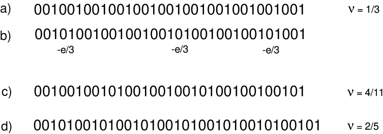
Figure 7: Quasiparticles and emergent Landau levels in the TT-limit. $(a)$ The TT-ground state 001 at $\nu=1/3$; in $(b)$ three quasielectrons with charge $-e/3$ are created by inserting 01 in three places. When one 01 is inserted for every third unit cell 001, the TT-ground state at $4/11$ is obtained $(c)$. In $(d)$ the 2/5 ground state is obtained by inserting one quasielectron for every unit cell 001. The ground states in $(c,d)$ can be interpreted as filling emergent Landau levels.

Of course, when decreasing the magnetic field and adding quasielectrons 01 to the 1/3 TT-state many other, infinitely many in fact, TT-ground states are obtained before the 2/5 state is reached, see Fig. 5. Among them are the states with unit cells $\{0_{2}1\}_{t_{2}}01$, see Fig. 6; these are just as 2/5 obtained by a condensation of quasielectrons in the 1/3 state albeit with a lower density of quasielectrons. However, these states have a filling factor with larger denominator and hence a smaller gap and are thus less stable to disorder and may not form in a given sample.

Continuing decreasing the magnetic field creates quasielectrons in the $2/5$-state by adding 01 which have charge $-e/5$ (adding 01 just before reaching 2/5 removes quasiholes of charge $e/5$). After having added 01 an additional $N$ times one reaches the 3/7 ground state with unit cell 0010101. Continuing the process gives all the TT ground states in the Jain sequence approaching $\nu=1/2$. Note that whereas the operation of inserting 01 is one and the same throughout this process, its interpretation in terms of quasiparticles varies: Near $p/(2p+1)$, adding 01 creates quasielectrons with charge $-e/(2p+1)$ and when approaching $(p+1)/(2p+3)$, adding 01 removes quasiholes of charge $e/(2p+3)$.

In the discussion above we started from the 1/3 state. However, due to the self-similar fractal structure established for the TT-ground states, it is clear that the procedure is general—it applies mutatis mutandis to any fraction $\nu=p/q$.

IV Transition to bulk

We have seen in the previous section that the TT-limit $L_{1}\rightarrow 0$ is remarkably simple but still rich and non-trivial. However, this is a limit that is most likely impossible to realize experimentally. Its raison d’$\rm{\hat{e}}$tre lies in what it says about the experimentally realizable two-dimensional bulk limit, $L_{1}\rightarrow\infty$,—this is the topic of this section.

We propose that the TT-ground state is the $L_{1}\rightarrow 0$ limit of a two-dimensional bulk QH state for any $\nu=p/q$, $q$ odd. If this QH state is the ground state (in the bulk) then it is adiabatically connected to the TT-state—there is in general no phase transition from the TT-state as $L_{1}$ goes from 0 to $\infty$. This statement may need clarification. When $L_{1}$ changes, the size of the physical system changes; normally when one talks about adiabatic continuity one has in mind that a parameter in the hamiltonian changes. However, all that is happening when $L_{1}$ changes is that the matrix elements $V_{km}$ change. Thus for any $L_{1}$, we can think of the problem as the infinite two-dimensional QH system with an interaction that depends on $L_{1}$. This interaction is unusual: for finite $L_{1}$ it is anisotropic, it becomes purely electrostatic in the TT-limit, and it cannot, presumably, be written as a real space interaction $V(r,L_{1})$. However, in the limit $L_{1}\rightarrow\infty$ it approaches the chosen isotropic electron-electron interaction, whereas it is exactly solvable in the TT-limit. Thus, we have the standard situation when adiabatic continuity can be discussed. In passing, we note that this point of view shows that the TT-states give an exact solution to the two-dimensional QH-problem albeit with a peculiar interaction.

We will present arguments for our proposal about adiabatic continuity below; the strength of these arguments varies with $\nu$. For the Laughlin states adiabatic continuity holds for a short-range pseudo-potential interaction, for the Jain states it can be strongly argued and for more general hierarchy states a case for it is emerging. In our opinion, the overall evidence for the correctness of the claim is convincing.

Apart from fractional QH states, there may of course be other ground states in the bulk. An example of this are Wigner crystals that are expected at low filling factors, in particular at $\nu=1/q$, for $q$ small enough. In these cases, there is a phase transition from the TT-state as $L_{1}$ increases.

The even denominator filling factors are special. For them we propose that there is always a phase transition from the gapped TT-state as $L_{1}$ increases. The suggestion is based on: 1) a detailed analysis of the $\nu=1/2$ case and 2) exact diagonalization of small systems. For $\nu=1/2$, we find a phase transition to a gapless Luttinger liquid that can be identified with a version of the Rezayi-Read state rr ; when $L_{1}$ increases further the state develops smoothly into the Rezayi-Read state that is believed to describe the system in the limit $L_{1}\rightarrow\infty$. Exact diagonalization of all $\nu=p/q$ with $q\leq 11$ shows that for each filling factor with even denominator there is an abrupt change in the ground state, where its quantum numbers change, as $L_{1}$ increases, whereas there is no such change for any odd denominator filling factor bk2 .

Below we first discuss the odd denominator hierarchy states, concentrating on the Laughlin and Jain fractions; results for more general hierarchy fractions are summarized. We then turn to even denominator fractions; we discuss the half-filled Landau level in detail and comment on general such fractions and on the difference between $\nu=1/2$ and $\nu=p/(2p+1)$. The TT-limit is useful also to analyze non-abelian states; we end by discussing the Moore-Read pfaffian state at $5/2$ as an example of this.

IV.1 Hierarchy states

We begin by comparing the qualitative properties of the TT-states and the bulk hierarchy states. First of all, both have a gap to excitations. Note that the crystalline TT-states have no phonons: once the boundary conditions, ie the flux through the torus, are fixed the lattice sites are fixed in space. Thus the TT-states are not the Wigner crystals expected in the quantum Hall system at low filling factor; these would have gapless phonons. Second, the TT-state and the bulk hierarchy state at $\nu=p/q$ both have quasiparticle excitations with charge $e^{*}=\pm e/q$. A further similarity is that the ground state degeneracy on the torus in both cases is $q$, but this is rather trivial as it is true for any state at $\nu=p/q$.

On the torus, the symmetries are the magnetic translations and the TT and Laughlin-Jain states have the same quantum numbers, $K_{\alpha}$, with respect to these. This follows since the former are the $L_{1}\rightarrow 0$ limit of the latter, see Appendix E.

The TT-state is inhomogeneous, whereas the bulk hierarchy state should be homogeneous—a property that is normally considered fundamental for the quantum Hall fluids. However, it should be noted that imposing periodic boundary conditions on the problem of electrons moving in a perpendicular magnetic field, ie considering the problem on a cylinder or a torus, implies that the continuous translational invariance present on the infinite plane, is broken, in one direction, to a discrete invariance, translation by one lattice constant $2\pi/L_{1}$, along the cylinder, see Appendix A. As a consequence, for any state on a finite cylinder or torus there will be ripples in the density that disappear completely only as the size of the torus goes to infinity haldanebook .

Furthermore, it should be noted that if one takes the alternative ”adiabatic” point of view where the TT-limit is just a change in the interaction $V_{km}$ in the infinite two-dimensional system (where the lattice constant vanishes), then the TT-state is homogeneous.

IV.1.1 Laughlin-Jain fractions

For the Laughlin and Jain filling fractions, $\nu=p/(2mp+1)$, explicit wave functions are known for the ground states as well as for the quasiparticle excitations—these allow us to further investigate the connection to the TT-states.

Rezayi and Haldane noted in 1994 that the $L_{1}\rightarrow 0$ limit of Laughlin’s wave function (at $\nu=1/3$) is the TT-state with unit cell 001 Haldane94 . This analysis can be generalized to general Jain states and also to quasiparticle excitations thereof. Taking the $L_{1}\rightarrow 0$ limit of these wave functions, one finds the TT-states and the quasiparticles of Sec. III bk2 . One direct consequence of this is that the TT-state has the same quantum numbers $K_{\alpha}$ as the Laughlin/Jain state. The details of this analysis are given in Appendix E.

On the plane, the Laughlin state at $\nu=1/(2m+1)$ is the unique ground state to a certain short range interaction and there is a gap to all excitations haldanebook ; trugman ; pokrovsky . Since this result on the plane is a consequence of the behavior of the wave function when two electrons approach each other it is natural that it holds in other geometries as well. This is indeed the case: For the short range interaction on the torus the Laughlin state is the unique ground state (up to the center of mass degeneracy) and there is a gap to all excitations for any circumference $L_{1}$. An explicit statement or proof of this has not, to the best of our knowledge, appeared, but it is implicit in Ref. Haldane94, . For a proof see Appendix F.

The transition from an inhomogeneous charge density wave state to a homogeneous-looking state as $L_{1}$ grows was studied in Haldane94 for the Laughlin $\nu=1/3$ state and a rapid crossover was found at $L_{1}\sim 6$. This crossover was recently studied numerically in detail by Seidel et al Lee05 . They confirm that there is no phase transition but an exponentially fast crossover to a virtually homogeneous state. That the Laughlin state spontaneously breaks the discrete translational symmetry on the thin cylinder has been rigorously proven by Jansen et al Jansen .

To conclude, we consider it firmly established that the TT ground states are adiabatically connected to the bulk QH states for the Laughlin fractions and that a strong case has been made for this being true also for the Jain fractions.

IV.1.2 Non-Jain hierarchy fractions

For the fractional QH states observed by Pan et al pan that are not of the Laughlin-Jain type discussed above no agreed upon wave functions exist. However, recently wave functions were constructed for all filling fractions in the hierarchy scheme that are obtained as repeated condensates of quasielectrons (as opposed to quasiholes) hierarchy ; conformal . These wave functions are obtained by a natural generalization of the conformal field theory construction of Jain’s composite fermion wave functions hans . The $L_{1}\rightarrow 0$ limit of the proposed wave functions are the TT ground states and the wave function at 4/11 has a large overlap with the exact ground state for small systems. We take this as a strong indication that the non-Jain hierarchy states in the bulk are also adiabatically connected to the TT ground states. Details of this conformal field theory construction of hierarchy wave functions will be presented elsewhere conformal . Wave functions at these fractions can also be constructed within the hierarchy scheme as condensates of quasiparticles greiter94 and as fractional QH states of composite fermions JainGoldman ; Quinn ; jain4over11 . For further discussion of these states, see Ref. lopez2, ; wojs, ; scomp2, ; pashitskii, .

IV.2 Even denominator fractions

So far we have discussed odd denominator filling factors and argued that the TT-states that are the ground states in the TT-limit are adiabatically connected to the two-dimensional bulk QH hierarchy states. In this section we discuss the even denominator filling factors. We begin by considering the half-filled Landau level; this case has been analyzed in detail and we believe it is representative for other gapless even denominators. (The gapped state at $5/2$ is discussed in Sec. IV.3.)

IV.2.1 Half-filled Landau level

In the half-filled lowest Landau level, $\nu=1/2$, a metallic, ie, gapless state is observed jiang . The composite fermion explanation for this behaviour is that each electron binds two flux quanta, thereby removing all the external magnetic flux. The state is then supposedly described by non-interacting, or weakly interacting, composite fermions in zero magnetic field, ie, by a free two-dimensional Fermi gas. This is also the picture that emerges from the mean field theory where the statistical magnetic field completely cancels the external magnetic field hlr . These descriptions successfully explain experimental data and constitute the main evidence for the correctness of the composite fermion idea. The microscopic wave function of composite fermion type describing the $\nu=1/2$ state was provided by Rezayi and Read rr —on the torus it reads rrhaldane

$$\mbox{$$}\Psi_{RR}={\rm det_{ij}}[e^{i{\bf k}_{i}\cdot{\bf R}_{j}}]\Psi_{\frac{1}{2}}\ \ \ ,$$ (25)

where ${\bf R}_{j}$ are the guiding center coordinates and $\Psi_{\frac{1}{2}}$ is the bosonic Laughlin state at $\nu=1/2$, see Appendix A. The wave function $\Psi_{RR}$ is not unique but depends on a set of parameters, ”momenta”, $\{{\bf k}_{i}\}$. In the two-dimensional bulk limit these are assumed to form a circular Fermi sea.

The TT-state at $\nu=1/2$ has unit cell 01, ie it is a state with one electron on every other site. This clearly minimizes the electrostatic repulsion, and hence is the ground state, in the TT-limit $L_{1}\rightarrow 0$. As any TT-state it has a gap to excitations and it has quasiparticles with charge $\pm e/2$. Clearly, this is very different from the gapless state that is observed in the two-dimensional bulk limit and is believed to be described by (25).

A gapless state does in fact exist also for small but finite $L_{1}$ and there is strong numerical evidence that this state develops without a phase transition into the gapless two-dimensional state described by (25). The first evidence for this was obtained in a numerical study of the QH system on a thin cylinder bkdmrg , using the density matrix renormalization group method white . At $\nu=1/2$, a sharp transition from the TT-state with a finite amplitude of the density oscillations to a virtually homogeneous state was observed at $L_{1}\sim 5$ (for a short-range interaction $V(\mathbf{r})=\nabla^{2}\delta(\mathbf{r})$) and there were indications of gapless excitations. This behaviour was dramatically different from other fractions such as $\nu=1/3$ where no transition was observed as $L_{1}$ was varied—the amplitude of the density wave decreased continuously as $L_{1}$ increased. The transition at $\nu=1/2$ takes place in a region where only the first few shortest-range terms $V_{km}$ are important. This made it possible to find an exact solution—ground state and low energy excitations—for a hamiltonian that is a very good approximation to the short-range interaction for $L_{1}\sim 5$ bk1 .

We now describe the exact solution, for details see Appendix G. Consider to start with a hamiltonian (1) that consists only of the shortest range hopping term, $V_{21}:\,1001\leftrightarrow 0110$. Define a restricted Hilbert space $\cal H^{\prime}$ by requiring that each pair of nearby sites $2p,2p+1$ contains exactly one electron, ie include the states $\uparrow=10$ and $\downarrow=01$, but not 00 or 11. Note that the interaction $V_{21}$ preserves the restricted Hilbert space $\cal H^{\prime}$. In spin notation, $1001\leftrightarrow 0110$ becomes $\uparrow\downarrow\leftrightarrow\downarrow\uparrow$ and hence the model with the shortest range hopping term $V_{21}$ is, within $\cal H^{\prime}$, equivalent to a nearest neighbour spin-1/2 $xy$-chain,

$$\mbox{$$}H_{xy}=V_{21}\sum_{p=0}^{N_{s}/2-1}(s^{+}_{p+1}s^{-}_{p}+s^{-}_{p+1}s^{+}_{p})\ \ \ ,$$ (26)

where $s^{+}_{p}=c^{\dagger}_{2p}c_{2p+1}$, $|\uparrow\rangle=s^{+}_{p}|\downarrow\rangle$, and $V_{21}>0$. Note that $s^{+}$ creates a neutral particle, a dipole. The hamiltonian (26) is diagonalized by mapping the spins to fermions, $\tilde{d}_{k}$, via a Jordan-Wigner transformation—the hamiltonian then becomes that of free one-dimensional fermions with nearest neighbor hopping.

Thus, within $\cal H^{\prime}$, the shortest range hopping term $V_{21}$ gives a one-dimensional free Fermi gas of neutral particles. But to make this a reasonable approximation to (1) for small but finite $L_{1}$ we must consider also the short-range electrostatic terms. Including the two shortest range such terms, $V_{10}$ and $V_{20}$, with relative strength $V_{10}=2V_{20}=2\alpha$ one finds that all states in $\cal H^{\prime}$ have the lowest possible electrostatic energy. There are states not in $\cal H^{\prime}$ (or $\cal H^{\prime}_{T}$) with the same electrostatic energy but a strong case can be made that the hopping term $V_{21}$ creates a gap to these ($\cal H^{\prime}$ contains the most hoppable states) bk1 ; this is also supported by the numerics discussed below. Thus, the low energy sector for the short-range hamiltonian

$$\mbox{$$}H_{sr} = \alpha\sum_{p=0}^{N_{s}-1}\hat{n}_{p}(2\hat{n}_{p+1}+\hat{n}_{p+2})$$ (27)

$$+ V_{21}\sum_{p=0}^{N_{s}/2-1}(s^{+}_{p+1}s^{-}_{p}+s^{-}_{p+1}s^{+}_{p})\ \ ,$$

where $\hat{n}_{p}=c^{\dagger}_{p}c_{p}$, is contained in $\cal H^{\prime}$ and is that of a free one-dimensional Fermi gas of neutral particles. The ground state is a filled Fermi sea

$$\mbox{$$}|GS\rangle=\prod_{|k|>\frac{\pi}{2}}\tilde{d}^{\dagger}_{k}|010101\ldots\rangle\ \ ,$$ (28)

and excitations out of this sea gives gapless neutral excitations. This provides an exact and explicit mapping of the low-energy sector of a system of interacting electrons in a magnetic field onto a system of non-interacting neutral particles, ie onto free particles that do not interact with the magnetic field.

We note that dipoles have many of the properties expected of composite fermions, most notably that they do not couple to the magnetic field. Earlier approaches to a microscopic theory in terms of dipoles were made by Read readearly ; read.5 , Murthy and Shankar ms , Pasquier and Haldane pasq , Lee dhlee and by Stern et al stern .

An important feature of the exact solution is that the number of dipoles is not conserved. These particles are neutral and their number is not tied to the number of electrons in the system as is the case for the composite fermions. For example, there are excitations where a single dipole is added to, or removed from, the Fermi sea. Moreover, the number of dipoles making up the Fermi sea in (28) is determined dynamically, ie by filling the negative energy dipole states; this leads to there being one dipole for every second electron. As this is a consequence of energetics, the number of dipoles presumably changes as $L_{1}$ increases. Assuming the ground state develops into a two-dimensional Fermi gas of dipoles as $L_{1}\rightarrow\infty$, this suggests that the number of dipoles, and hence the Fermi momentum, is determined dynamically rather than being simply given by the number of electrons. In this context we note that the Fermi momentum measured in surface acoustic wave experiments Willettreview disagrees with the mean field theory result which follows from that the number of composite fermions in the Fermi sea is equal to the number of electrons hlr .

The solvable case is a good approximation for a small finite $L_{1}$. For the real-space short-range interaction $V(\mathbf{r})=\nabla^{2}\delta(\mathbf{r})$, $V_{10}=2V_{20}=2\alpha$ corresponds to $L_{1}=2\pi/\sqrt{2\ln 2}=5.3$. The short-range hopping term is then $V_{21}=\frac{3}{8}\alpha$, whereas the leading ignored terms are small: $V_{30}=\frac{9}{128}\alpha$ and $V_{31}=\frac{1}{32}\alpha$. This is close to the solvable point.

Longer range hopping terms in (1) will in general not preserve the subspace $\cal H^{\prime}$. However, since there is a gap to states not in $\cal H^{\prime}$, the effect of small such terms can be included perturbatively in an effective spin-1/2 hamiltonian that acts within $\cal H^{\prime}$. To zeroth order the effective hamiltonian is

$$H_{eff}=\sum_{p,n}[V_{2n,1}(s^{+}_{p+n}s^{-}_{p}+s^{-}_{p+n}s^{+}_{p})-\Delta_{2n}s^{z}_{p}s^{z}_{p+n}]\ ,$$ (29)

where $s^{z}_{p}=\frac{1}{2}(n_{2p-1}-n_{2p})$ and $\Delta_{2n}$ is given in (19). In particular, this effective hamiltonian, $H_{eff}$, contains an Ising term $s^{z}_{p}s^{z}_{p+n}$ that changes the non-interacting Fermi gas to an interacting Luttinger liquid with interaction parameter $K\neq 1$. If such terms come with large coefficients, they may cause a phase transition that opens up a gap; the results below strongly indicate that this does not happen in this system. In higher order perturbation theory, one gets increasingly more complicated spin-1/2 models containing renormalized quadratic as well as higher order terms. However, our numerical calculations suggest that these higher order terms may be very small for a range of $L_{1}$—we find that the projection of the exact ground state of the Coulomb interaction on $\cal H^{\prime}$ is virtually unity in the ”solvable” region $5.3<L_{1}<8$ as discussed below.

We have numerically identified the state obtained in exact diagonalization in the solvable region with the exact solution (28). We continuously varied $V_{km}$ from the values that give the exact solution to values that correspond to a $L_{1}$ in this region and verified that the ground state develops continuously without any level crossing. Whereas $H_{xy}$ gives a qualitative understanding, we suggest that $H_{eff}$ gives a quantitatively very accurate description of the low energy sector within this region. Thus we conclude that the exact solution is stable in a finite neighborhood of the solvable point where it develops into an interacting gapless one-dimensional model, a Luttinger liquid.

However, the perturbative argument for this is of course restricted to hamiltonians close to the solvable one—when $L_{1}$ increases, hopping terms of increasing range and with large coefficients will appear—leading to a hamiltonian that is very different from (27) and that definitely does not preserve the restricted hilbert space $\cal H^{\prime}$. To investigate this region we compared the ground states obtained in exact diagonalization with the Rezayi-Read states (25) bk2 .

The plane waves in (25) are periodic on the torus, with our normalization this means that $k_{\alpha}$ are integers. A straightforward calculation shows that these momenta determine the conserved quantum numbers $K_{\alpha}$ of the state:

$$\mbox{$$}K_{\alpha}=\sum_{i=0}^{N_{e}-1}k_{i\alpha}\ \ {\rm mod}((1+\delta_{1\alpha})N_{e})\ \ ,$$ (30)

where $k_{i\alpha}$ is the momentum of particle $i$. We represent a state (25) by displaying its set of momenta as in Fig. 8. The Rezayi-Read state is invariant under a rigid translation of the momenta, $k_{i\alpha}\rightarrow k_{i\alpha}+(1+\delta_{1\alpha})n_{\alpha}$, where $n_{\alpha}$ are integers kinvariance (this so-called $K$-symmetry was first noted by Haldane). Since the conserved quantum numbers are defined modulo $(1+\delta_{1\alpha})N_{e}$, see Appendix A, they are invariant under this translation. The rigid translation $k_{i\alpha}\rightarrow k_{i\alpha}+\delta_{1\alpha}$ changes the quantum numbers but corresponds to a translation of the center of mass only.

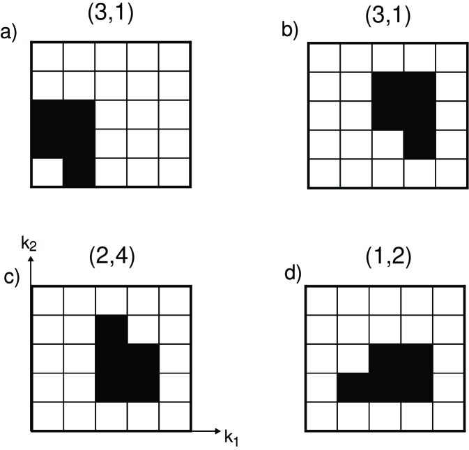
Figure 8: Examples of Fermi seas of momenta $\{k_{i\alpha}\}$ for $N_{e}=5$. For each sea the conserved momenta $(K_{1},K_{2})$ are displayed. $a)$ and $b)$ are related by a translation that corresponds to K-invariance, and have the same quantum numbers; they describe the same state. $c)$ is one of three new states obtained from $a)$ by reflections in the $x$- and $y$-axes. These four states have different quantum numbers and are degenerate ground states for $5.3<L_{1}<L_{2}$, cf Fig. 9; translating the corresponding Fermi seas one step in the $x$-direction gives the remaining four ground states. $d)$ is obtained from $c)$ by a rotation by $\pi/2$; it is one of the ground states when $5.3<L_{2}<L_{1}$.

Fig. 9 shows results for the ground state at $\nu=1/2$ for various $L_{1}$ for $N_{e}=4-9$ electrons which interact with an unscreened Coulomb interaction. For all $N_{e}$ there is a sharp transition from the TT-state to a new ground state at $L_{1}\approx 5.3$. (In cases where the ground state is degenerate, cf Fig. 8, only one representative is considered in Fig. 9.) As $L_{1}$ increases further there are additional transitions. The next transition occurs also at approximately the same $L_{1}$ for all $N_{e}$; this is particularly clear when an even/odd effect is ignored and one considers only say the odd $N_{e}$. There are additional transitions for larger $L_{1}$—but the number and positions of these depend on the number of particles. Each of the states at $L_{1}>5.3$ has a very large overlap with a Rezayi-Read wave function for some choice of Fermi sea of parameters $\{{\bf k}_{i}\}$. Overlaps are around or above 0.99 and they are essentially constant in each region. The Fermi seas develop in a systematic way from an elongated shape at small $L_{1}$ to a circular one as $L_{1}$ increases. It is as circular as it can be when $L_{1}=L_{2}=\sqrt{4\pi N_{e}}$ for the small number of particles considered in Fig. 9.

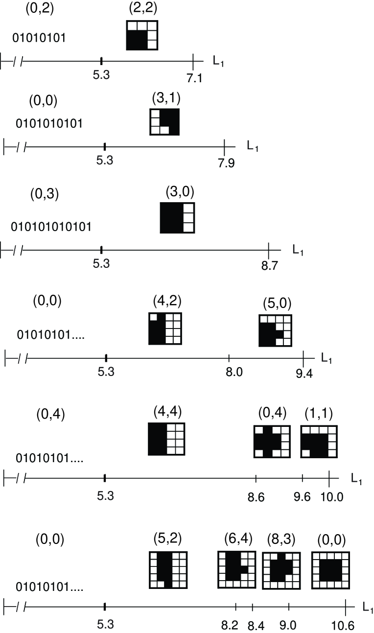
Figure 9: Ground states and corresponding quantum numbers $(K_{1},K_{2})$ at $\nu=1/2$ as a function of $L_{1}$ for 4 to 9 electrons (from top to bottom) ($K_{1}$ is given ${\rm mod}(N_{e})$). The results are obtained in exact diagonalization, using an unscreened Coulomb interaction. Marked $L_{1}$ denote transitions to new ground states. For $L_{1}<5.3$ the (virtually exact) ground state is the TT-state, whose unit cell is 01 when $L_{1}\rightarrow 0$. In each region $L_{1}>5.3$, the state is identified with a Rezayi-Read state with the displayed Fermi sea of momenta. The overlap with the Rezayi-Read state is around or above 0.99 for all $N_{e}$ (in all regions). The phase diagram is symmetric about $L_{1}=L_{2}=\sqrt{4\pi N_{e}}$, which are the largest marked $L_{1}$ in the figure.

From the numerical results for a small number of electrons we extract the following interpretation for an infinite number of electrons (ie for $L_{2}\rightarrow\infty$) and varying $L_{1}$. At $L_{1}\approx 5.3$ there is a phase transition from the gapped TT-state, with unit cell 01 as $L_{1}\rightarrow 0$, to a gapless state well described by the exact solution or equivalently by the Rezayi-Read state with a special choice of momenta $\{{\bf k}_{i}\}$ forming an elongated Fermi sea. Perturbative corrections will turn this state into a Luttinger liquid with $K\neq 1$ in the region $5.3<L_{1}<8$. When $L_{1}$ increases further the Fermi sea deforms continuously approaching a circular sea as $L_{1}\rightarrow\infty$. The transitions for $L_{1}>5.3$ in Fig. 9 are not phase transitions but rather level crossings to similar states—such crossings are expected to occur in a gapless system. These transitions correspond to small changes of the momenta in the Rezayi-Read wave function, typically only one momentum is changed at each transition. Consider a finite $L_{1}>5.3$ and $L_{2}\rightarrow\infty$. This is a one-dimensional system, and since it is obtained from the Rezayi-Read state that we have identified with the gapless exact solution by a continuous change of momenta $\{{\bf k}_{i}\}$, we strongly believe that it is gapless. On general grounds, it should then be a Luttinger liquid—or possibly several Luttinger liquids. Further support for it being gapless is obtained from the fact that, as $L_{1}\rightarrow\infty$, it approaches the two-dimensional case which is generally believed to be gapless. Of course, this is expected to be a gapless two-dimensional system—a free two-dimensional Fermi gas. It is an interesting and unresolved question how the smooth transition from the Luttinger liquid at $L_{1}>5.3$ to the two-dimensional gapless system occurs. In any case, our interpretation of the exact diagonalization results is that this transition is smooth—there is no phase transition as $L_{1}$ varies above 5.3.

IV.2.2 Other even denominator fractions

For even denominator fractions other than $\nu=1/2$ we have much less to say; however, we suggest that the half-filled Landau level is typical and that a similar scenario holds for other even denominator fractions. There is some numerical evidence for this. We have performed exact diagonalisation, for various $L_{1}$, for all filling factors $\nu=p/q\leq 1$ with $q\leq 11$. All even denominator fractions are similar to $\nu=1/2$ in that there are transitions from the TT-state to new states with different quantum numbers as $L_{1}$ grows. For the odd denominator fractions, on the other hand, no such transition is ever seen—the ground states develop smoothly from the TT-states.

IV.2.3 Even versus odd denominators

How can we understand, within the approach presented here, that even and odd denominators are so different? To this question we have no complete answer but we will offer some insights obtained from the case when the shortest range hopping term, $V_{21}$, is included, ie when $L_{1}$ is small but finite.

Let us consider $\nu=1/2$ and the Jain sequence $\nu=p/(2p+1)$ that approaches this fraction as $p$ grows—why is 1/2 gapless whereas the others have a gap? In the former case there is a phase transition from the gapped TT-state to a gapless state whereas in the latter case the gapped TT-state develops continuously into the bulk quantum Hall system as $L_{1}\rightarrow\infty$. To some extent this difference can be understood by comparing the TT-states. As we have noted, they are the states that minimize the electrostatic repulsion $V_{k0}$ and thus are the ground states as $L_{1}\rightarrow 0$. When $L_{1}$ increases, hopping terms $V_{km}$, $m\neq 0$, become important. Consider the first hopping term $V_{21}$ that enters as $L_{1}$ increases. The TT-state at $\nu=1/2$ with unit cell 01 is annihilated by $V_{21}$, ie it is a non-hoppable state. There is a transition to a ground state that is more hoppable, thus lowering the kinetic energy. The ground state in the exact solution (28) contains the maximally hoppable basis state with unit cell 1001. For $\nu=1/2$, it is the competition between the electrostatic terms, that favor the TT-state, and the hopping terms that favor other states, such as 1001, that leads to the phase transition at $L_{1}=5.3$. For $\nu=1/3$, the TT-state has unit cell 001; by construction this minimizes the electrostatic repulsion. But it is also the most hoppable state with respect to the hopping term $V_{21}$. Thus, in this case there is no competition between electrostatic repulsion and hopping—they collaborate rather than compete—and hence there is no phase transition. Of course, this does not explain why longer range hopping terms that are important for larger $L_{1}$ do not cause a transition. This argument extends to any filling fraction $\nu=p/(2p+1)$ in the Jain sequence that approaches $1/2$. In spite of the fact that the TT-state for large $p$ looks very similar to the TT-state at $\nu=1/2$, which is non-hoppable, the TT-state at $\nu=p/(2p+1)$ is very hoppable. In fact, inserting a single extra hole in the $\nu=1/2$ TT-state gives a very hoppable state.

Thus we see that for $\nu=1/2$ there is a doubling of the ”unit cell”, $01\rightarrow 1001$, that does not happen at 1/3. This generalizes to other filling fractions and we suggest that the most hoppable state at odd denominators is simply the TT-state with unit cell ${\bf C}$, whereas at even denominators it is the state with doubled unit cell ${\bf C}^{T}{\bf C}$, where ${\bf C}^{T}$ is the transpose of ${\bf C}$. This is in agreement with the doubling of the period in the ”parent state” for even denominators noted by Su su2 . It is an open question how these considerations relate to the explanation by Tao and Wu taowu .

We end this section by pointing out an intriguing possible relation to the Haldane conjecture for the presence of gaps in spin chains haldanegap . The gapless half-filled Landau level is, in the exact solution above, mapped onto a spin 1/2 system. The low-energy sector is obtained by grouping the sites in pairs with one electron in each pair. Attempting a similar mapping of the low energy sector at 1/3, when the leading hopping term $V_{21}$ is included, suggests grouping the sites in sets of three with one electron in each group. This gives three states per group, and a mapping to a spin one chain. This leads us to speculate that the existence (absence) of a gap at odd (even) denominators in the QH system is related to the Haldane conjecture for spin chains that says that integer spin chains have a gap whereas half-integer chains are gapless.

The arguments given here are at present restricted to the QH system with a small, but finite, $L_{1}$ since only the shortest range hopping term $V_{21}$ is included. However, in this context it is interesting to note that the ground state obtained at $\nu=1/3$ with a hamiltonian that only includes $V_{21}$, without any electrostatic terms, has a 98% overlap with the Laughlin state for six electrons at $L_{1}=7$ juha . Of course, when the number of particles, and $L_{1}$, increases this overlap will drop as longer range hopping terms become important.

IV.3 Non-abelian states—Moore-Read state at 5/2

So far we have seen that the gapped hierarchy states as well as the gapless $\nu=1/2$ state exist for small $L_{1}$. This limit is relevant also for non-abelian states, where a simple understanding of the nontrivial degeneracies and fractional charges appear we06 ; haldaneAPS ; seidel06 . As an example of this we discuss the Pfaffian state proposed by Moore and Read mr . This gapped state is a competitor to the gapless Rezayi-Read state (25) for a half-filled Landau level. It was suggested greiter as a candidate for the observed gapped $\nu=5/2$ state 52exp . There is now numerical evidence that this suggestion is indeed correct morf ; rrhaldane ; moller .

The Moore-Read state is peculiar: It has a six-fold degeneracy on the torus rather than only the two-fold implied by the filling factor, it has excitations with charge $\pm e/4$ rather than $\pm e/2$ as one would expect for a gapped state at half-filling and most surprisingly a state with $2n$ quasiholes has degeneracy $2^{n-1}$ for fixed quasiparticle positions. Moreover, these quasiparticles have non-abelian fractional statistics. These properties were obtained by an intricate relationship to conformal field theory. It has been proposed that the topological and non-abelian properties of these states can be used for constructing a topologically-protected decoherence-free quantum computer Freedman . The Moore-Read state is the exact ground state of a certain local three-body interaction greiter ; rrhaldane . This is true on a torus for any $L_{1}$ and can be used to show that the ground states in the TT-limit are the TT-states with unit cells $01$ and $0110$, ie the unique states where the distance between all pairs of next nearest neighbor electrons is maximal. Applying $T_{2}$ we see that $01$ is two-fold degenerate whereas $0110$ is four-fold degenerate—this gives the six-fold degeneracy of the ground state. By joining strings of $01$ and $0110$ ground states it follows, using the Su-Schrieffer counting argument, that the domain walls are quasiparticles with charge $\pm e/4$. In this way one can construct a general state with $k$ quasiholes and $2n-k$ quasielectrons and show that it has degeneracy $2^{n-1}$ for fixed positions of the excitations. Thus, again the qualitative properties of the state are obtained on the thin torus. Moreover, the manifest particle-hole symmetry of the Fock space formulation allows the construction of a general state of quasielectrons and quasiholes.

The Moore-Read pfaffian state is not particle-hole symmetric; conjugating the six degenerate states give six orthogonal states, the anti-pfaffian states, that are believed to describe a different phase of matter apf1 ; apf2 . The TT-limits $01$ and $0110$ of the pfaffian states are on the other hand particle-hole symmetric and hence the anti-pfaffian states have the same TT-limit. For small $L_{1}$, the difference shows up in subleading terms emiljuha .

The analysis of the non-abelian states in the TT-limit has recently been generalized to more general parafermionic states parafermionic . Again a simple understanding of the quasiparticles as domain walls between degenerate ground states gives the non-trivial degeneracies haldaneAPS ; read06 ; weunpublished .

Appendix A One Landau level on torus

We here give details for a single Landau level on a torus, which we assume has lengths $L_{1},L_{2}$ in the $x$ and $y$-directions respectively. The complete analysis was given by Haldane; this includes an arbitrariness in a choice of two-dimensional lattice Haldane85 ; Haldane85PRL , see also Ref. fradkin ; read . As we are interested in the mapping to a one-dimensional system, we restrict ourselves to the corresponding lattice; this allows for an explicit and simple construction.

In Landau gauge, ${\bf A}=By\hat{\bf x}$, the hamiltonian for a free electron becomes, in units where $\hbar=c/eB=1$,

$$\mbox{$$}H=\frac{1}{2m}({\bf p}-\frac{e}{c}{\bf A})^{2}=-\frac{1}{2m}[(\partial_{x}-iy)^{2}+\partial_{y}^{2}]\ .$$ (31)

The invariance under continuous spatial translations in the $y$-direction has now been broken to discrete translations, $y\rightarrow y+n2\pi/L_{1}$, where $n$ is an integer: The gauge transformation $\psi\rightarrow e^{i\Lambda({\bf r})}\psi$, ${\bf A}\rightarrow{\bf A}+\frac{c}{e}\vec{\nabla}\Lambda$ must be periodic $e^{i\Lambda(x+L_{1})}=e^{i\Lambda(x)}$ and hence translations $y\rightarrow y+a$, where $a$ is a constant, can be compensated for in $A_{x}$, and hence in (31), by the gauge transformation $e^{-iax}$ only if $a$ is a multiple of the lattice constant $2\pi/L_{1}$.

The magnetic translation operators $\hat{t}_{\alpha},\alpha=1,2$, that translate an electron a distance $L_{\alpha}/N_{s}$ in the $\alpha$-direction are

$$\mbox{$$}\hat{t}_{1}=e^{(L_{1}/N_{s})\partial_{x}}\ ,\ \ \ \hat{t}_{2}=e^{(L_{2}/N_{s})(\partial_{y}+ix)}\ ,$$ (32)

where $N_{s}=L_{1}L_{2}/(2\pi)$ is the number of flux quanta through the surface; the operators obey

$$\mbox{$$}\hat{t}_{1}\hat{t}_{2}=e^{2\pi i/N_{s}}\hat{t}_{2}\hat{t}_{1}\ \ .$$ (33)

The Landau level preserving ”guiding center” coordinates used in the Read-Rezayi state (25) are defined as:

$$\mbox{$$}R_{ix}=(2\pi/L_{1})(x_{i}-i\partial_{y_{i}})\ ,\ \ R_{iy}=(2\pi/L_{2})i\partial_{x_{i}}\ \ .$$ (34)

The states

$$\mbox{$$}\psi_{k} = e^{-2(k\pi/L_{1})^{2}}\hat{t}_{2}^{k}\psi_{0}\ ,\ \ \ k=0,1,...,N_{s}-1\ ,$$ (35)

$$\psi_{0} = \pi^{-1/4}L_{1}^{-1/2}\sum_{n}e^{inL_{2}x}e^{-(y+nL_{2})^{2}/2}\ \ ,$$ (36)

form a basis of one-particle states in the lowest Landau level. $\psi_{k}$ is a periodic gaussian located along the line $y=-2\pi k/L_{1}$ and is a $\hat{t}_{1}$ eigenstate, $\hat{t}_{1}\psi_{k}=e^{i2\pi k/N_{s}}\psi_{k}$. Letting $c^{\dagger}_{k}$ create an electron in state $\psi_{k}$, $\{c_{k},c_{m}^{\dagger}\}=\delta_{km}$, maps the Landau level onto a one-dimensional lattice model with lattice constant $2\pi/L_{1}$, see Fig. 1. A basis of many-particle states is given by $|n_{0},n_{1},\dots n_{N_{s}-1}\rangle$, where $n_{k}=0,1$ depending on whether site $k$ is empty or occupied by an electron; alternatively the state is described by the positions $\{k_{1},k_{2},...,k_{N_{e}}\}$ of the particles.

On the cylinder, the single-particle states in Landau level $p$ are

$$\psi_{pk}(\mathbf{r}) = (\sqrt{\pi}2^{p}p!L_{1})^{-1/2}e^{-2(\pi k/L_{1})^{2}}$$ (37)

$$\times H_{p}(y+k\frac{2\pi}{L_{1}})e^{2\pi ikz/L_{1}}e^{-y^{2}/2}\ \ ,$$

where $z=x+iy$ and $H_{p}$ is the $p:$th Hermite polynomial. Here, the lowest Landau level wave functions, $\psi_{0k}\equiv\psi_{k}$, are obtained by setting $n=0$ in (35).

Consider the electron gas at filling fraction $\nu=p/q$, where $p$ and $q$ are relatively prime integers and the number of electrons, $N_{e}=N_{s}p/q$, is an integer. The operators $T_{\alpha}=\prod_{i}^{N_{e}}\hat{t}_{i\alpha}$, (where $\hat{t}_{i\alpha}$ translates electron $i$) commute with $H$ and, since $T_{\alpha}^{N_{s}}=1$, the eigenvalues are $e^{2\pi iK_{\alpha}/N_{s}},K_{\alpha}=0,...,N_{s}-1$. However, $T_{1}$ and $T_{2}$ do not commute:

$$\mbox{$$}T_{1}T_{2}=e^{2\pi ip/q}T_{2}T_{1}\ \ ;$$ (38)

thus $T_{1}$ and $T_{2}^{q}$ commute and $\{H,T_{1},T_{2}^{q}\}$ is a maximal set of commuting operators. $T_{2}$ changes $K_{1}$ by $N_{e}$ and leaves the energy unchanged. Hence, each energy eigenstate is $q$-fold degenerate and we can choose to characterize it by the smallest $K_{1}$. Thus, the energy eigenstates are characterized by a two-dimensional vector $K_{\alpha}=0,...,N_{s}/q-1$; the eigenvalues of $T_{1}$ and $T_{2}^{q}$ are $e^{2\pi iK_{1}/N_{s}}$ and $e^{2\pi iqK_{2}/N_{s}}$ respectively. The vector $K_{\alpha}$ corresponds to, but is different from, Haldane’s vector $k_{\alpha}$ in Ref. Haldane85PRL, , which characterizes the relative motion of the electrons only.

The TT-state that is the ground state at $\nu=p/q=N_{e}/N_{s}$ in the TT-limit is a single Slater determinant $\{k_{1},k_{2},\dots k_{N_{e}}\}$ with eigenvalues

$$T_{1}\Psi_{TT}=e^{2\pi i\sum_{i}k_{i}/N_{s}}\Psi_{TT}$$

$$T_{2}^{q}\Psi_{TT}=(-1)^{p(N_{e}-p)}\Psi_{TT}\ \ \ .$$ (39)

These TT-states are continuous limits of QH hierarchy states, hence the latter have the same quantum numbers.

The second quantized electron-electron interaction is

$$H=\sum_{k_{1},k_{2},k_{3},k_{4}=0}^{N_{s}-1}\!\!\!V_{k_{1}k_{2}k_{3}k_{4}}c^{\dagger}_{k_{1}}c^{\dagger}_{k_{2}}c_{k_{3}}c_{k_{4}}\ \ ,$$ (40)

where the matrix elements are

$$V_{k_{1}k_{2}k_{3}k_{4}}=\frac{1}{2}\int\int d^{2}r_{1}d^{2}r_{2}\psi_{k_{1}}^{*}(\mathbf{r}_{1})\psi_{k_{2}}^{*}(\mathbf{r}_{2})$$

$$\times V(|\mathbf{r}_{1}-\mathbf{r}_{2}|)\psi_{k_{3}}(\mathbf{r}_{2})\psi_{k_{4}}(\mathbf{r}_{1})\ ;$$ (41)

here both the one-particle states $\psi_{k}$ and the interaction $V(\mathbf{r})$ are periodic and the integration is over the torus with sides $L_{1}$ and $L_{2}$ yoshioka . For the Coulomb interaction, $V(\mathbf{r})=\sum_{s,t}\frac{e^{2}}{\epsilon|\mathbf{r}+sL_{1}\hat{x}+tL_{2}\hat{y}|}$, the matrix elements become

$$V_{k_{1}k_{2}k_{3}k_{4}}\!=\!\frac{\delta^{\prime}_{k_{1}+k_{2},k_{3}+k_{4}}}{2L_{1}L_{2}}\!\!\!\sum_{(q_{1},q_{2})\neq(0,0)}\delta^{\prime}_{k_{1}-k_{4},q_{1}L_{1}/2\pi}$$

$$\times\frac{2\pi e^{2}}{\epsilon q}e^{-\frac{q^{2}}{2}-i(k_{1}-k_{3})\frac{q_{2}L_{2}}{N_{s}}},$$ (42)

where $\delta^{\prime}$ is the periodic Kronecker delta function (with period $N_{s}$) and $q_{i}=\frac{2\pi n_{i}}{L_{i}}$, $n_{i}=0,\pm 1,\ldots$. The divergent $\mathbf{q}=0$ term is excluded in (42); it would be cancelled by adding a positive (neutralizing) background charge. By taking advantage of the translation invariance and momentum conservation one can re-write the hamiltonian as in (40):

$$\mbox{$$}H=\!\!\sum_{n=0}^{N_{s}-1}\sum_{|m|<k\leq\frac{N_{s}}{2}}\frac{V_{km}}{\!1\!+\!\delta_{k,\frac{N_{s}}{2}}\!\!}c^{\dagger}_{n+m}c^{\dagger}_{n+k}c_{n+k+m}c_{n}\ ,$$ (43)

where

$$V_{km}=V_{n+m,n+k,n+m+k,n}-V_{n+m,n+k,n,n+m+k}$$

$$+V_{n+k,n+m,n,n+m+k}-V_{n+k,n+m,n+m+k,n}\ .$$ (44)

It follows that the matrix elements are real and $V_{km}=V_{k,-m}$, which assures that $H$ is hermitian. Moreover, from the periodicity $V_{km}=V_{k+nN_{s},m+n^{\prime}N_{s}}$ and the symmetry $V_{km}=V_{-k,m}$ of (42) follows that $V_{km}=V_{N_{s}-k,m}$; this is used to express the excitation energies in terms of $V_{km}$ in Sec. III.1.

A general many-body eigenstate of a translation invariant hamiltonian can be separated into a center of mass piece, a relative part and a gaussian factor. Prime examples are the Laughlin wave functions at filling fraction $\nu=1/{t_{1}}$ Haldane85

$$\Psi_{\frac{1}{t_{1}}}=\vartheta^{m/{t_{1}}+(N_{s}-{t_{1}})/2{t_{1}}}_{({t_{1}}-N_{s})/2}({t_{1}}\sum_{i}z_{i}/L_{1}|i{t_{1}}L_{2}/L_{1})$$

$$\times\prod_{i<j}\vartheta_{1}((z_{i}-z_{j})/L_{1}|iL_{2}/L_{1})^{t_{1}}e^{-\frac{1}{2}\sum_{i}y_{i}^{2}}\ .$$ (45)

Here $\vartheta_{b}^{a}(z|\tau)=\sum_{n}e^{i\pi\tau(n+a)^{2}+2\pi i(n+a)(z+b)}$ (sum over all integers) are the Jacobi theta functions and $\vartheta_{1}\equiv\vartheta_{1/2}^{1/2}$ is the standard odd theta function. $m=0,1,\ldots,{t_{1}}-1$ gives the ${t_{1}}$ degenerate states that differ by a translation of the center of mass only. QH hierarchy wave functions are given for the torus geometry in Ref. toruswfs, . The non-abelian Moore-Read state is another example of a state that is known on the torus pfafftorus .

Appendix B Ground states as $L_{1}\rightarrow 0$

We here prove that the relaxation procedure in Sec. III gives the ground state. The energy $E$ of a state $|n_{0}n_{1}\dots n_{N_{s}-1}\rangle$ with $N_{e}$ electrons can be written in terms of the interaction between the $N_{e}(N_{e}-1)$ different ordered pairs of electrons. Let $\alpha=1,\dots,N_{e}$ number the electrons along the circle in positive direction, cf Fig. 4. Consider an ordered pair of electrons $(\alpha,\alpha+k)$ and let $E_{\alpha,\alpha+k}$ be the interaction energy between these electrons taken along the path, in the positive direction, from $\alpha$ to $\alpha+k$. Each ordered pair is obtained exactly ones by letting $k=1,\dots N_{e}-1$, hence the energy becomes

$$\mbox{$$}E=\sum_{k=1}^{N_{e}-1}\sum_{\alpha=1}^{N_{e}}E_{\alpha,\alpha+k}\equiv\sum_{k=1}^{N_{e}-1}E^{(k)}\ \ ,$$ (46)

where $E^{(k)}$ is the interaction energy for all pairs that are $k$:th nearest neighbors.

The crucial observation is that it is possible to minimize the energies $E^{(k)}$ separately for an interaction that obeys the concavity condition (6) hubbard . This condition implies that the interaction energy of one electron with two other electrons that have fixed positions is minimized if the first electron is as close to the midpoint between the fixed electrons as possible, ie if the distances to the two fixed electrons differ by at most one lattice constant, see Fig. 3.

We will show that the state given by the relaxation procedure in Sec. III minimizes all the energies $E^{(k)}$ and hence it minimizes $E$ and is the ground state.

The energy $E^{(k)}$ is minimized as follows. Let $a^{(k)}_{\alpha}$ denote the distance between electrons $\alpha$ and $\alpha+k$. Then $\sum_{\alpha=1}^{N_{e}}a^{(k)}_{\alpha}=kN_{s}$ (in units of the lattice constant), hence the average distance between two electrons that are $k$:th nearest neighbors is $(a^{(k)}_{\alpha})_{ave}=kN_{s}/N_{e}=k/\nu$. This is a trivial consequence of the periodic boundary conditions on the circle and holds for any state $|n_{0}n_{1}\dots n_{N_{s}-1}\rangle$ with $N_{e}$ electrons. Using the concavity condition (6) as in Fig. 3 it follows that $E^{(k)}$ is minimized if the distances $a^{(k)}_{\alpha}$ between the electrons in all the pairs of $k$:th nearest neighbors are as equal as possible, ie if $a^{(k)}_{\alpha}$ for each fixed $k$ and $\alpha=1,\dots N_{e}$ differ by one lattice constant at most. First we note that if $k=p$ then the average distance is an integer, $(a^{(p)}_{\alpha})_{ave}=p/\nu=q$. $E^{(p)}$ is thus minimized if and only if the distance from any electron to its the $p:$th neighbor is $q$; thus the state is periodic with a unit cell of length $q$ containing $p$ electrons. Consider now the pairs of $k$:th nearest neighbors. Before moving the electrons to the closest sites, the separations between the electrons in the pairs are all equal, $a^{(k)}_{\alpha}|_{0}=k/\nu$, $\alpha=1,\ldots,N_{e}$. Each electron is then moved at most 1/2 lattice constant and hence $|a^{(k)}_{\alpha}-k/\nu|<1$; note that this is strictly less than one since two electrons never move 1/2 lattice constant each. It then follows that $|a^{(k)}_{\alpha}-a^{(k)}_{\beta}|<2$ for any $\alpha,\beta$. But this difference is by construction an integer, hence $|a^{(k)}_{\alpha}-a^{(k)}_{\beta}|\leq 1$. This proves that the unit cell constructed by the relaxation procedure minimizes $E^{(k)}$, for any $k$, and hence gives the ground state.

We believe the ground state solution is unique, up to the center of mass degeneracy, and have verified this in special cases but have not proven it for general $\nu$.

Appendix C Quasiparticle charge

We here show that the quasiparticles proposed in Sec. III have the expected charges $e^{*}=\pm e/q$ at $\nu=p/q$. Letting $\nu_{i}=p_{i}/q_{i}$, we find from (III.1)

$$\mbox{$$}p_{i}=t_{i}p_{i-1}+\alpha_{i}p_{i-2}\ \ ,\ \ \ q_{i}=t_{i}q_{i-1}+\alpha_{i}q_{i-2}\ \ ,$$ (47)

where $\alpha_{i}=1$ ($-1$) is for the upper (lower) equation in (III.1). Consider the quasiparticles at $\nu_{n}$, ie in the ground state with unit cell ${\bf C}^{(n)}$. The charge of the insertion ${\bf C}^{(n-1)}$ is determined using the Su-Schrieffer counting argument. Insert ${\bf C}^{(n-1)}$ in $q_{n}$ well separated places and remove $q_{n-1}$ unit cells ${\bf C}^{(n)}$. This preserves the number of sites $N_{s}$ but changes the number of electrons by $\delta N_{e}=q_{n}p_{n-1}-q_{n-1}p_{n}$. Thus the charge of the insertion ${\bf C}^{(n-1)}$ is $e^{*}=-e\delta N_{e}/q_{n}$. From (47), we find

$$\mbox{$$}q_{i}p_{i-1}-q_{i-1}p_{i}=-\alpha_{i}(q_{i-1}p_{i-2}-q_{i-2}p_{i-1})\ \ .$$ (48)

Iterating this we find

$$q_{n}p_{n-1}-q_{n-1}p_{n} = \prod_{i=2}^{n}(-\alpha_{i})(q_{1}p_{0}-q_{0}p_{1})$$ (49)

$$= (-1)^{n}\prod_{i=2}^{n}\alpha_{i}\ \ \ ,$$

where the last step follows from the explicit forms for $\nu_{0}$ and $\nu_{1}$ in Sec. III. This gives $\delta N_{e}=\pm 1$ and hence the insertion ${\bf C}^{(n-1)}$ at $\nu_{n}=p_{n}/q_{n}$ has charge $e^{*}=\pm e/q_{n}$. The conjugate $\overline{{\bf C}^{(n-1)}}$ obviously has the opposite charge $e^{*}=\mp e/q_{n}$ since ${\bf C}^{(n-1)}\overline{{\bf C}^{(n-1)}}={\bf C}^{(n)}$ is the unit cell of the ground state and hence is neutral (with respect to the ground state).

Appendix D Excitation energy as $L_{1}\rightarrow 0$

We here provide background material for the calculation of the energy of a particle-hole pair in Sec. III. We consider explicitly the ordering in (16), but the arguments generalize immediately to (17). First we show that the replacement (15), which creates a nearest neighbor particle-hole pair, simply amounts to moving one electron one lattice constant in the ground state unit cell ${\bf C}^{(n)}$. Using (III.1), and the definition of $\overline{{\bf C}^{(n-1)}}$, it is straightforward to show that ${\bf C}^{(n-1)}\overline{{\bf C}^{(n-1)}}$ and $\overline{{\bf C}^{(n-1)}}{\bf C}^{(n-1)}$ only differ in the ordering of ${\bf C}^{(n-2)}$ and $\overline{{\bf C}^{(n-2)}}$; thus the original problem is mapped onto the equivalent problem at the previous level in the hierarchy. Iterating this all the way to level one we can use the explicit form of the unit cells ${\bf C}^{(1)}$ and $\overline{{\bf C}^{(1)}}$ to verify that one electron has moved on lattice constant only.

To prove the induction step, we first consider the case where the last condensation leading to ${\bf C}^{(n)}$ is of the first type in (III.1). Using $\overline{{\bf C}^{(n-1)}}={\bf C}^{(n-1)}_{t_{n}-1}{\bf C}^{(n-2)}$ we find

$${\bf C}^{(n-1)}\overline{{\bf C}^{(n-1)}}={\bf C}^{(n-1)}{\bf C}^{(n-1)}_{t_{n}-1}{\bf C}^{(n-2)}$$

$$={\bf C}^{(n-1)}_{t_{n}-1}{\bf C}^{(n-2)}\overline{{\bf C}^{(n-2)}}{\bf C}^{(n-2)}$$ (50)

and

$$\overline{{\bf C}^{(n-1)}}{\bf C}^{(n-1)}={\bf C}^{(n-1)}_{t_{n}-1}{\bf C}^{(n-2)}{\bf C}^{(n-1)}$$

$$={\bf C}^{(n-1)}_{t_{n}-1}{\bf C}^{(n-2)}{\bf C}^{(n-2)}\overline{{\bf C}^{(n-2)}}\ ,$$ (51)

which clearly only differ in the ordering of ${\bf C}^{(n-2)}$ and $\overline{{\bf C}^{(n-2)}}$. For the second type in (III.1) we identify $\overline{{\bf C}^{(n-1)}}={\bf C}^{(n-1)}_{t_{n}-2}\overline{{\bf C}^{(n-2)}}$ and find

$${\bf C}^{(n-1)}\overline{{\bf C}^{(n-1)}}={\bf C}^{(n-1)}_{t_{n}-1}\overline{{\bf C}^{(n-2)}}$$

$$={\bf C}^{(n-1)}_{t_{n}-2}{\bf C}^{(n-2)}\overline{{\bf C}^{(n-2)}}\ \overline{{\bf C}^{(n-2)}}$$ (52)

and

$$\overline{{\bf C}^{(n-1)}}{\bf C}^{(n-1)}={\bf C}^{(n-1)}_{t_{n}-2}\overline{{\bf C}^{(n-2)}}{\bf C}^{(n-1)}$$

$$={\bf C}^{(n-1)}_{t_{n}-2}\overline{{\bf C}^{(n-2)}}{\bf C}^{(n-2)}\overline{{\bf C}^{(n-2)}}\ ,$$ (53)

which also differ only in the ordering of ${\bf C}^{(n-2)}$ and $\overline{{\bf C}^{(n-2)}}$. This concludes the proof.

Note that the creation of a nearest neighbor pair as in (15) amounts to a translation of a single unit cell assuming periodic boundary conditions on this cell. The finite distance case (16) amounts to repeating this for $s$ consecutive unit cells, ie translating them with periodic boundary conditions on each cell separately (this is actually equivalent to translating all $s$ cells together with periodic boundary conditions on the set). Since one electron is moved one lattice constant for each unit cell, $s$ electrons forming a lattice with lattice constant $q$ are moved rigidly one lattice constant in (16).

We now derive the expression (18) for the energy of a particle-hole pair. To do so we divide the electrons into three disjoint sets $A,B,C$, where set $A$ consists of the $s$ electrons that moved under (16) (these electrons are all in the region between the particle and hole). We now note that the action of (16) can alternatively be achieved by translating first all unit cells so that the particle-hole region agrees with the one obtained using (15), and then translating all unit cells outside the particle-hole pair region back to their initial positions. The first step does not change any interactions while the second step moves one electron per unit cell outside of the particle-hole pair region—these electrons form set $B$. Again, the electrons in set $B$ form a regular lattice with lattice constant $q$. Set $C$ consists of the remaining electrons. From the first construction follows that all the relative distances between the particles in the set $B\cup C$ are unchanged and from the second that the same holds true for the particles in $A\cup C$; in addition all relative distances within each of the three sets are unchanged.

The energy of a state is the sum over the interaction energies of all pairs of electrons, and the energy of an excitation relative to the ground state is the sum of the change of all such terms. It follows from the above that a pair energy can change only if one particle is in $A$ and the other is in $B$. In the ground state the electrons in $A\cup B$ form a lattice with lattice constant $q$; the particle-hole excitation is obtained by translating a string of $s$ adjacent of these electrons one lattice constant. This shows which pair energies change; adding the contributions gives (18).

We now show that the nearest neighbor particle-hole-pair in (15) is the lowest energy excitation at a given filling fraction $\nu=p/q$. The ground state is the state that minimizes the interaction energy between all pairs of $k$:th nearest neighbors $E^{(k)}$ in (46) for all $k=1,...,N_{e}-1$. For an excited state at least one $E^{(k)}$ must be non-minimal. We divide the excited states into two categories: the states where $E^{(np)}$, $n=1,2,\ldots,(N_{e}-1)/p$, are minimal and those where they are not. The former are the periodic states with exactly $p$ electrons on any $q$ consecutive sites. The nearest neighbor particle-hole excitation is obtained by moving one electron one lattice constant and is hence a non-periodic state. We have seen above that only the distances to the $np$:th neighbors change, hence only $E^{(np)}$ change for this excitation. Furthermore, the change in $E^{(np)}$ is the smallest possible, as implied by the concavity condition (5) (see also Fig. 3), thus the nearest neighbor particle-hole pair is the smallest energy non-periodic excitation. The periodic excitations have a much higher energy since they violate the ground state conditions within each unit cell, thus their energy diverge with the size of the system.

Appendix E Laughlin and Jain states as $L_{1}\rightarrow 0$

Here we show that the $L_{1}\rightarrow 0$ limit of the Laughlin and Jain states, and of their quasiparticle excitations, are the TT-states and quasiparticles given in Sec. III. For the ground state at $\nu=1/3$ this was shown in Ref. Haldane94, .

For simplicity, we give the argument on the cylinder rather than on the torus. Expressing the wave functions in terms of $z$ and $y$, the projection onto the lowest Landau level is achieved by moving $y$ to the left and letting $y\rightarrow i\partial_{z}$, where the derivative should not act on the factor $e^{-y^{2}/2}$; this is a straightforward generalization of the method given by Girvin and Jach proj . Throughout this Appendix the overall factor $e^{-\sum_{i}y_{i}^{2}/2}$ is omitted in all wave functions as it is not affected by the projection.

The Jain state at $\nu=p/(2mp+1)$ on the cylinder takes the form jainrev2

$$\mbox{$$}\Psi_{\frac{p}{2mp+1}}={\rm Det}[\hat{\eta}_{j}(\hat{\bf r}_{i})\gamma_{i}]\ \ \ ,$$ (54)

where

$$\mbox{$$}\gamma_{i}=\prod_{j\neq i}(\beta_{i}-\beta_{j})^{m}\ ,\ \ \ \ \ \beta_{i}=e^{2\pi iz_{i}/L_{1}}\ \ .$$ (55)

$\eta_{i}({\bf r}_{j})$ is a Landau level wave function $\psi_{nk}({\bf r}_{j})$ (37)

$$\mbox{$$}\psi_{nk}({\bf r})\propto e^{-2(\frac{k\pi}{L_{1}})^{2}}H_{n}(y+k\frac{2\pi}{L_{1}})\beta^{k}\ \ ,$$ (56)

and $\hat{\eta}_{i}(\hat{\bf r}_{j})$ is the operator obtained from this wave function by letting $y_{j}\rightarrow i\partial_{z_{j}}$. The $\eta_{i}({\bf r}_{j})$ are chosen as the one-particle states in the $p$ lowest Landau levels. (Note that $\partial_{z}$ acts within one term in the determinant; this corresponds to Jain’s second method of projecting onto the lowest Landau level jainrev2 .)

Consider first the Laughlin states, $\nu=1/(2m+1)$, then $\eta$ are the lowest Landau level wave functions

$$\mbox{$$}\eta({\bf r})=\psi_{0k}\propto e^{-2(\frac{k\pi}{L_{1}})^{2}}\beta^{k}\ \ .$$ (57)

(Only a single Slater determinant of one-electron states survives when $L_{1}\rightarrow 0$, hence we can ignore multiplicative $L_{1}$-independent constants in the wave functions.) In this case there is no dependence on $y$ and no need to project onto the lowest Landau level; (54) of course gives the Laughlin wave function on the cylinder thouless

$$\mbox{$$}\Psi_{\frac{1}{2m+1}}=\prod_{i<j}(\beta_{i}-\beta_{j})^{2m+1}\ \ .$$ (58)

We want to translate this wave function to an occupation number basis, ie to write it as a sum of Slater determinants of one-electron states. This is achieved by noting that $\beta^{k}$ corresponds to the unique lowest Landau level one-electron state $\psi_{k}$ (37). Thus, replacing

$$\mbox{$$}\beta^{k}\rightarrow e^{2(\frac{k\pi}{L_{1}})^{2}}\psi_{0k}$$ (59)

in (54), or in this case in (58), the Slater determinants can be read off; these states all have the same $K_{1}=\sum k_{i}$. Because of the factor in (59) the state with the largest $\sum_{i}k_{i}^{2}$ dominates when $L_{1}\rightarrow 0$. This is clearly the state obtained by first choosing one $k$ as large as possible, then the next as large as possible and so on (all $k_{i}$ are different because of the Pauli principle). It is easy to see that the Tao-Thouless state with unit cell $0_{2m}1$ is contained in (58) and that it is the state which maximizes $\sum_{i}k_{i}^{2}$ for the given $K_{1}=\sum_{i}k_{i}$. Hence, it is the limit of $\Psi_{\frac{1}{2m+1}}$ as $L_{1}\rightarrow 0$. The quasiparticles are discussed below.

We now turn to the Jain states, where $p>1$. The determinant in (54) then contains the wave functions, $\psi_{nk}$, $n=0,1,\dots,p-1$ of the $p$ lowest Landau levels. Projecting $\psi_{nk}({\bf r}_{i})\gamma_{i}$ onto the lowest Landau level, $y\rightarrow i\partial_{z}$, gives

$$\mbox{$$}\hat{\psi}_{nk}(\hat{\bf r}_{i})\gamma_{i} \propto e^{-2(\frac{k\pi}{L_{1}})^{2}}H_{n}(i\partial_{z_{i}}+k\frac{2\pi}{L_{1}})\beta_{i}^{k}\gamma_{i}$$ (60)

$$= e^{-2(\frac{k\pi}{L_{1}})^{2}}\beta_{i}^{k}H_{n}(i\partial_{z_{i}})\gamma_{i}\ \ .$$

Defining

$$\mbox{$$}\alpha_{it}\equiv m\frac{2\pi}{L_{1}}\sum_{j\neq i}(\frac{\beta_{i}}{\beta_{i}-\beta_{j}})^{t}\ ,$$ (61)

we have, using $\partial_{z_{i}}\beta_{i}=\frac{2\pi i}{L_{1}}\beta_{i}$,

$$\mbox{$$}\partial_{z_{i}}\gamma_{i} = \alpha_{i1}\gamma_{i}\ ,$$

$$\partial_{z_{i}}\alpha_{it} = t(\alpha_{it}-\alpha_{i,t+1})\ \ \ .$$ (62)

Since the Hermite polynomial $H_{n}$ is an $n$:th grade polynomial in $\partial_{z_{i}}$ it follows that

$$\mbox{$$}H_{n}(i\partial_{z_{i}})\gamma_{i} = m_{in}\gamma_{i}\ \ ,$$ (63)

where $m_{in}$ is a polynomial in $\alpha_{it}$.

Forming the determinant in (54), using (63) and noting that $\prod_{i}\gamma_{i}=\prod_{i\neq j}(\beta_{i}-\beta_{j})^{m}=\prod_{i<j}(\beta_{i}-\beta_{j})^{2m}\equiv\Psi_{\frac{1}{2m}}$ is the $\nu=1/2m$ bosonic Laughlin state, one finds that (54) can be written as

$$\mbox{$$}\Psi_{\frac{p}{2mp+1}}\propto{\rm Det}[M_{\{nk\}i}]\Psi_{\frac{1}{2m}}\ ,$$ (64)

where

$$\mbox{$$}M_{\{nk\}i}=\beta_{i}^{k}m_{in}\ .$$ (65)

Here, $\{nk\}$ denotes the first index of the matrix $M$: $n=0,1\dots p-1$ numbers the Landau levels and $k=0,1,\dots N-1$ numbers the states in each level. The second index numbers the electrons, $i=1,2,\dots pN$.

We have expressed $\Psi_{\frac{p}{2mp+1}}$ in terms of $\beta$ and can now translate it to the occupation number basis using (59). Just as above, the leading order term will be the one that maximizes $\sum_{i}k_{i}^{2}$. One finds that this is obtained by taking the state with maximal $\sum_{i}k_{i}^{2}$ in $\Psi_{\frac{1}{2m}}$—this is the TT-state with unit cell $0_{2m-1}1$. An element $\beta_{i}^{k}$ in $M$ acts as an operator on the occupation number states in $\Psi_{\frac{1}{2m}}$, translating particle $i$ to the right $k$ steps, ie increasing its momentum by $k$. The elements $\beta^{k}_{i}m_{in}$, $n=1,2,\dots$ also move the $i$:th particle $k$ steps to the right just as $\beta^{k}_{i}$ alone does. This is because $m_{in}$ is a polynomial in $\alpha_{it}$ and it can be seen that such terms do not change the highest power of $\beta_{i}$ when acting on $\Psi_{\frac{1}{2m}}$, cf (61). Considering the action of a term in the determinant it follows that it will move groups of $p$ electrons $k$ steps to the right, where $k=0,1,\dots,N-1$. We see that $\sum_{i}k_{i}^{2}$ is maximized if the $p$ leftmost electrons, ie the ones with smallest $k_{i}$, are not moved, then, moving to the right, the next $p$ electrons are moved one step to the right and so on until finally the rightmost set of $p$ electrons, the ones with the largest $k_{i}$, are moved $N-1$ steps to the right. This gives the TT-state with unit cell $0_{2m}1(0_{2m-1}1)_{p-1}$.

To clarify the limit, we consider $\nu=2/5$ explicitly. In this case, $p=2$, $m=1$, and thus there are $2N$ particles—$N$ in each of the two effective Landau levels. From (64) and (65) it follows that we can write the wave function as

$$\mbox{$$}\!\!\!\!\Psi_{\frac{2}{5}}\!=\!\!\left|\!\begin{array}[]{cccc}\beta_{1}^{N-1}m_{1,1}&\beta_{2}^{N-1}m_{2,1}&\!\ldots\!&\beta_{2N}^{N-1}m_{2N,1}\\ \beta_{1}^{N-2}m_{1,1}&\beta_{2}^{N-2}m_{2,1}&\!\ldots\!&\beta_{2N}^{N-2}m_{2N,1}\\ \vdots&\vdots&\!\ddots\!&\vdots\\ m_{1,1}&m_{2,1}&\!\ldots\!&m_{2N,1}\\ \beta_{1}^{N-1}m_{1,0}&\beta_{2}^{N-1}m_{2,0}&\!\ldots\!&\beta_{2N}^{N-1}m_{2N,0}\\ \vdots&\vdots&\!\ddots\!&\vdots\\ m_{1,0}&m_{2,0}&\!\ldots\!&m_{2N,0}\end{array}\!\right|\!\Psi_{\frac{1}{2}}\!.$$ (73)

To maximize $\sum_{i}k_{i}^{2}$ we pick one $k_{i}$, ie one of the powers of $\beta_{i}$, as large as possible in the expansion of (73). This is achieved if and only if the power of $\beta_{i}$ is maximized both in the determinant and in $\Psi_{\frac{1}{2}}$. The highest power in the determinant is $N-1$ and in $\Psi_{\frac{1}{2}}$ it is $2(2N-1)$, thus the maximal $k_{i}$ is $5N-3$. Next, we need to find the second highest power. Again the power from the determinant is $N-1$ (note that a given term in the determinant can include factors such as $\beta_{1}^{N-1}\beta_{2}^{N-1}$) while it is $2(2N-2)$ from the Jastrow factors $\Psi_{\frac{1}{2}}$, thus the total power is $5N-5$. Next one finds that the determinant can only contribute a power $N-2$ and that the highest power coming from $\Psi_{\frac{1}{2}}$ is $2(2N-3)$. Continuing this one finds that the maximal $k_{i}$ in the determinant decreases by one for every second particle while it always decreases by two in $\Psi_{\frac{1}{2}}$. This gives the unit cell $00101$. From this example, the general procedure given above should be clear.

It is now straightforward to generalize the analysis above to quasiparticle states. In Jain’s approach, these are constructed by replacing one of the one-electron states in (54) by a state in a higher empty Landau level. Assuming the levels involved are the highest occupied and the lowest empty ones, $\psi_{p-1,k}\rightarrow\psi_{p,q}$, this amounts to replacing $\beta_{i}^{k}m_{i,p-1}$ by $\beta_{i}^{q}m_{i,p}$ (for all $i$ and fixed $k,q$) in the matrix $M$ in (65). This has the effect of moving $0_{2m-1}1$ from one place to another in the TT-ground state, ie of creating a particle-hole pair of excitations with charge $\pm e/(2m+1)$, cf Sec. III B. The position of the excitation depends on $k$ and $q$, and in particular one of them can be put at the end of the cylinder.

Appendix F Laughlin state on cylinder

The Laughlin state is the exact and unique ground state for a certain short-range interaction and there is a gap to all excitations haldanebook ; trugman ; pokrovsky . The proofs were formulated using spherical or disk geometry. The essential ingredient is, however, only the short-distance behavior of the wave functions when two electrons approach each-other—thus it may be regarded as obvious that the result holds also on the cylinder (or torus) for arbitrary circumference $L_{1}$; this result is in fact implicit in Ref. Haldane94, . There has, however, been some controversy on this point and as the result is important in establishing that the state develops continuously without a phase transition from the TT-state for small $L_{1}$ to the two-dimensional bulk Laughlin state as $L_{1}\rightarrow\infty$, we here explicitly show that the Laughlin state is the exact and, up to rigid translations, unique ground state on a cylinder for a short range interaction and that there is a gap to all excitations for any $L_{1}$. Our argument follows closely that of Trugman and Kivelson trugman .

A fermionic many-particle state in the lowest Landau level is a sum of Slater determinants

$$\Psi(\{\mathbf{r}_{i}\})\! = \!\sum_{\{k_{i}\}}a_{\{k_{i}\}}\det_{i,j}(\psi_{k_{i}}(\mathbf{r}_{j}))$$ (74)

$$= f(\{\beta_{i}\})e^{-\sum_{j}y_{j}^{2}/2}\ \ ,$$

where $\psi_{k}$ are lowest Landau level single particle states on the cylinder (37) and $\beta_{i}=e^{2\pi iz_{i}/L_{1}}$. The range $\Delta k$ of the momenta $k_{i}$ restricts the system in space and thus depends on the number of particles and the filling factor $\nu=p/q$. The filling factor is the number of electrons divided by the number of sites, $\nu=N_{e}/(\Delta k+1)$. Because of the $q$-fold translational degeneracy, $\Delta k=\Delta\tilde{k}-(q-1)$, where $\Delta\tilde{k}$ is the range of momenta in $f$. $f$ is an anti-symmetric polynomial in $\beta_{i}$, hence it contains the Jastrow factor $J=\prod_{i<j}(\beta_{i}-\beta_{j})$. The problem of minimizing the energy of a specific electron-electron interaction in the lowest Landau level is thus reduced to finding the polynomial $f$ that gives the lowest energy given the above constraints. (This is in complete analogy with the problem in the plane where the polynomial is instead in terms of $z_{i}$.)

Consider now the repulsive interaction

$$V(\mathbf{r})=\sum_{s=0}^{\infty}V_{s}(\mathbf{r})=\sum_{s=0}^{\infty}c_{s}b^{2s}\nabla^{2s}\delta_{p}(\mathbf{r})\ \ ,$$ (75)

where $b$ is the range of the interaction, $c_{s}$ are positive constants, and $\delta_{p}(x,y)=\sum_{n}\delta(x+nL_{1},y)$ is the periodic delta-function. The leading term, $\langle\,V_{0}\,\rangle$, is identically zero for any fermionic state. By assuming $b\rightarrow 0$ only the leading non-vanishing term in (75) contributes to the energy $E=\langle\,V(\mathbf{r})\,\rangle$.

The expectation value of $V_{s}$ is

$$\langle\,V_{s}\,\rangle=4c_{s}b^{2s}\sum_{i<j}\prod_{k\neq i,j}\int d^{2}\mathbf{r}_{k}d^{2}Zd^{2}z\delta^{2}_{p}(z)\partial^{s}{\bar{\partial}}^{s}(\Psi^{*}\Psi),$$ (76)

where we have integrated by parts , and changed to relative coordinates for the pair that is affected by the interaction, $z=z_{i}-z_{j},Z=(z_{i}+z_{j})/2$, $\partial=\partial/\partial z$. Performing the derivatives in the integrand gives

$$\mbox{$$}\partial^{s}{\bar{\partial}}^{s}(\Psi^{*}\Psi)=e^{-\sum_{k\neq i,j}y_{k}^{2}/2}e^{(z-\bar{z})^{2}/16}e^{(Z-\bar{Z})^{2}/4}\$$

$$\times[\partial^{s}f{\bar{\partial}}^{s}{\bar{f}}+\sum_{r,t=0,r+t\neq 2s}^{s}\alpha_{rt}\partial^{r}f{\bar{\partial}}^{t}{\bar{f}}]\ \ ,$$ (77)

for some $\alpha_{rt}$. For $s=1$, only the first term contributes to $\langle\,V_{1}\,\rangle$ since $f(0)=0$, and this term is non-negative $\langle\,V_{1}\,\rangle\geq 0$. $\langle\,V_{1}\,\rangle=0$ if and only if $\partial f|_{z=0}=0$; if this is the case then only the first term in (F) for $s=2$ contributes to $\langle\,V_{2}\,\rangle$ and $\langle\,V_{2}\,\rangle\geq 0$, the equality sign holding if and only if $\partial f|_{0}=\partial f^{2}|_{0}=0$. This continues to any order in $s$ and we have that $\langle\,V_{t}\,\rangle=0$ for $t=1,2,\dots s$, and $\langle\,V_{s+1}\,\rangle\geq 0$, if and only if $\partial^{t}f|_{0}=0$ for $t=1,2,\dots s$. This means that $f$ vanishes at least as fast as $z^{s+1}$ when $z\rightarrow 0$, and since this holds for any $z_{i}-z_{j}=z$ and $f$ is an antisymmetric polynomial in $\beta_{i}$, it follows that $f$ contains at least $s+1$ powers of the Jastrow factor: $f=J^{s+1}\tilde{f}$, where $\tilde{f}$ is a new polynomial in $\beta_{i}$.

Consider the truncated interaction $V^{(s)}(\mathbf{r})=\sum_{t=0}^{s}V_{t}(\mathbf{r})$. We have found that a state has vanishing energy if and only if $f=J^{s+1}\tilde{f}$. These are the ground states: All other states have positive energy since, as $b\rightarrow 0$, only the first non-zero $\langle\,V_{t}\,\rangle$ contributes and this is non-negative according to the discussion above.

For $\tilde{f}=1$, $f$ is the Laughlin state at filling factor $\nu=1/(s+1)$ which thus is a ground state; it is unique since any non-constant polynomial $\tilde{f}$ decreases the filling factor. This proves the proposition.

On the torus, an analogous argument implies that the zero-energy states must contain a factor $\prod_{i<j}\vartheta_{1}((z_{i}-z_{j})/L_{1}|iL_{2}/L_{1})^{s+1}$, which together with the boundary conditions specify the Laughlin state on the torus (45) uniquely up to the $s+1-$fold center of mass degeneracy.

Appendix G Exact solution at $\nu=1/2$

Here we give details of the exact diagonalization of the short-range hamiltonian (27)bk1 .

The crucial part in (27) is the hopping term $V_{21}$. However, we begin by considering the electrostatic part $H_{sr}|_{V_{21}=0}$, which has eigenstates with fixed charges, $|n_{0}n_{1}...n_{N_{s}-1}\rangle$. The energy of such a state is

$$E_{0}=\alpha(\frac{N_{s}}{2}+n_{111}+n_{000})\ \ ,$$ (78)

where, $n_{111}\,(n_{000})$ is the number of 3-strings, ie strings consisting of three nearby electrons (holes) in $n_{0}n_{1}...n_{N_{s}-1}$. Thus there is a degenerate ground state manifold ${\cal H}_{0}$ consisting of all states where at most two electrons or two holes are next to each other. The energy $E_{0}$ follows by writing the right hand side of (78) in terms of $\hat{n}_{i}$ and comparing to (27).

To proceed we define a subspace ${\cal H}^{\prime}$ of the full Hilbert space by requiring each pair of sites $(2p,2p+1)$ to have charge one (acting with $T_{2}$ gives an equivalent grouping of the sites $(2p-1,2p)$ and a corresponding subspace $\cal H^{\prime}_{T}$). As we will demonstrate below, $H_{sr}$ preserves the subspace $\cal H^{\prime}$ and can be exactly diagonalized in this subspace giving non-interacting neutral fermions. Note that ${\cal H}^{\prime}\subset{\cal H}_{0}$, thus any state in ${\cal H}^{\prime}$ has the lowest possible electrostatic energy. As argued in the main text and in Ref. bk1, , ${\cal H}^{\prime}$ also contains the low-energy sector of the hopping term $V_{21}$ and thus of the hamiltonian $H_{sr}$ (27).

There are two possible states for a pair of sites in $\cal H^{\prime}$:

$$|\downarrow\rangle\equiv|01\rangle\ ,\ \ |\uparrow\rangle\equiv|10\rangle\ \ ;$$ (79)

introducing the spin operators

$$s^{+}_{p}=c^{\dagger}_{2p}c_{2p+1}\ ,\ \ \ s^{-}_{p}=c^{\dagger}_{2p+1}c_{2p}\ \ ,$$ (80)

where $p=0,1,\dots N_{e}-1$, we have

$$s^{+}|\downarrow\rangle=|\uparrow\rangle\ ,\ \ \ s^{-}|\uparrow\rangle=|\downarrow\rangle\ \ .$$ (81)

On states in $\cal H^{\prime}$, $s^{+},\,s^{-}$ describe hard core bosons—they commute on different sites but obey anti-commutation relations on the same site

$$[s^{-}_{i},s^{+}_{j}]=[s^{-}_{i},s^{-}_{j}]=[s^{+}_{i},s^{+}_{j}]=0\ ,\ \ \ i\neq j$$

$$\{s^{-}_{i},s^{+}_{i}\}=1,\ \ \{s^{-}_{i},s^{-}_{i}\}=\{s^{+}_{i},s^{+}_{i}\}=0\ \ ,$$ (82)

and $H_{sr}$ is the nearest neighbor spin 1/2 $xy$-chain,

$$H_{sr}=\alpha N_{e}+V_{21}\sum_{p=0}^{N_{e}-1}[s^{+}_{p+1}s^{-}_{p}+s^{-}_{p+1}s^{+}_{p}]\ ,$$ (83)

where $s^{\pm}_{N_{e}}\equiv s^{\pm}_{0}$ and $V_{21}>0$. We diagonalize $H_{sr}$ following the standard procedure, see eg Ref. fradkin, ; schulz, . Expressing the (hard core) bosons in terms of fermions $d$ using the Jordan-Wigner transformation,

$$s^{-}_{p}=K_{p}d_{p},\ \ \ K_{p}=e^{i\pi\sum_{j=0}^{p-1}d^{\dagger}_{j}d_{j}}\ ,$$ (84)

the hamiltonian becomes that of free fermions,

$$H_{sr}=\alpha N_{e}+V_{21}\sum_{p=0}^{N_{e}-2}[d^{\dagger}_{p+1}d_{p}+d^{\dagger}_{0}K_{N_{e}-1}d_{N_{e}-1}+hc]\ ,$$ (85)

when restricted to $\cal H^{\prime}$. The explicit $K$-factor can be ignored for $N_{e}\rightarrow\infty$ Lieb ; however, $H_{sr}$ can be diagonalized exactly also for finite $N_{e}$ including this $K$-factor by noting that, in this term, $K_{N_{e}-1}=(-)^{N_{\uparrow}+1}$, where $N_{\uparrow}$ is the number of up spins in the state. Thus

$$H_{sr}=\alpha N_{e}+V_{21}\sum_{p=0}^{N_{e}-1}[d^{\dagger}_{p+1}d_{p}+d^{\dagger}_{p}d_{p+1}]\ ,$$ (86)

where $d_{N_{e}}\equiv(-)^{N_{\uparrow}+1}d_{0}$. Since $N_{\uparrow}$ is conserved by $H_{sr}$, we can diagonalize $H_{sr}$ by the Fourier transformation

$$d_{j} = \frac{1}{\sqrt{N_{e}}}\sum_{k}e^{ijk}\tilde{d}_{k}\ ,$$

$$\tilde{d}_{k} = \frac{1}{\sqrt{N_{e}}}\sum_{j=0}^{N_{e}-1}e^{-ijk}{d}_{j}\ ,$$ (87)

where for $N_{\uparrow}$ odd

$$k\frac{N_{e}}{2\pi} = 0,\pm 1,\pm 2,\dots\pm(\frac{N_{e}}{2}-1),\frac{N_{e}}{2}\ \ \ {\rm for}\ N_{e}\ {\rm even}$$

$$k\frac{N_{e}}{2\pi} = 0,\pm 1\pm 2,\dots\pm(\frac{N_{e}}{2}-\frac{1}{2})\ \ \ {\rm for}\ N_{e}\ {\rm odd}\,;$$ (88)

whereas for $N_{\uparrow}$ even, $k$ is shifted by $-\pi/N_{e}$:

$$k\frac{N_{e}}{2\pi}\rightarrow k\frac{N_{e}}{2\pi}-\frac{1}{2}\ \ .$$ (89)

Note that this implies that different sets of momenta $k$ are used in states obtained when acting with an even or odd number of operators $\tilde{d}^{\dagger}$ on the Fock vacuum

$$\prod_{j=1}^{N_{\uparrow}}\tilde{d}^{\dagger}_{k_{j}}|010101\dots\rangle\ \ .$$ (90)

It can be shown that (90) are eigenstates of $T_{1}$ and $T_{2}^{2}$ with eigenvalues

$$K_{1} = -N_{\uparrow}+N_{e}^{2}$$

$$K_{2} = -\frac{N_{e}}{2\pi}\sum_{j=1}^{N_{\uparrow}}k_{j}+\frac{N_{e}(N_{e}-1)}{2}\ \ .$$ (91)

The hamiltonian becomes

$$H_{sr}=\alpha N_{e}+2V_{21}\sum_{k}\cos{k}\ \tilde{d}^{\dagger}_{k}\tilde{d}_{k}\ .$$ (92)

The ground state is obtained by filling the lowest energy states respecting the condition that an odd (even) number of states must be filled when $k$ takes the values in (G) (is shifted by $-\pi/N_{e}$). For $N_{e}$ even, a unique ground state is obtained by filling all the negative energy states

$$|GS\rangle=\prod_{|k|>\frac{\pi}{2}}\tilde{d}^{\dagger}_{k}|010101\ldots\rangle\ .$$ (93)

For $N_{e}$ odd, the ground state is obtained by filling all the negative states except for the highest, or alternatively all the negative states and the lowest positive state. This leads to a four-fold degenerate ground state (in $\cal H^{\prime}$). This degeneracy corresponds to reflections of the Fermi sea in horizontal and vertical lines that give new Fermi seas for odd $N_{e}$ but not for even $N_{e}$, see Figs. 8, 9.

This solves the problem in $\cal H^{\prime}$ and, by action of $T_{2}$, in $\cal H^{\prime}_{T}$. When $N_{e}\rightarrow\infty$, the ground state has energy

$$E/N_{e}=\alpha-\frac{2V_{21}}{\pi}$$ (94)

per electron. The excitations are neutral particle and/or hole excitations out of this Fermi sea. They have, according to (80), a natural interpretation in terms of dipoles and in the limit $N_{e}\rightarrow\infty$ the excitations become gapless. All of the electric charge sits in the Fock vacuum, $|010101\ldots\rangle$, while the quasi-particles $\tilde{d}_{k}$ that build up the ground state are neutral.

A straightforward calculation shows that $\langle c^{\dagger}_{m}c_{n}\rangle=\frac{1}{2}\delta_{mn}$, when $N_{e}\rightarrow\infty$ , hence

$$\mbox{$$}\langle\rho(\mathbf{r})\rangle = \sum_{m,n}\psi^{*}_{m}(\mathbf{r})\psi_{n}(\mathbf{r})\langle c_{m}^{{\dagger}}c_{n}\rangle$$ (95)

$$= \frac{1}{2}\sum_{m}\psi^{*}_{m}(\mathbf{r})\psi_{m}(\mathbf{r})\ \ \ .$$

Thus this state is homogenous in occupation space (this is not the case for the TT-states), and hence approximately homogeneous in real space for any $L_{1}$, becoming completely homogeneous when $L_{1}\rightarrow\infty$ (as is the case also for the TT-states).

References

- (1)
- (2) K.v. Klitzing, G. Dorda and M. Pepper, Phys. Rev. Lett. 45, 494 (1980).
- (3) D.C. Tsui, H.L. Störmer and A.C. Gossard, Phys. Rev. Lett. 48, 1599 (1982).
- (4) B.I. Halperin, Phys. Rev. Lett. 52, 1583 (1984).
- (5) D.P. Arovas, J.R. Schrieffer, and F. Wilczek, Phys. Rev. Lett. 53, 722 (1984).
- (6) R.B. Laughlin, Phys. Rev. B. 23, 5632 (1981).
- (7) B.I. Halperin, Phys. Rev. B. 25, 2185 (1982).
- (8) R.B. Laughlin, Phys. Rev. Lett. 50, 1395 (1983); R.B. Laughlin in The Quantum Hall Effect, eds. R.E. Prange, and S.M. Girvin, (Springer-Verlag, New York, 1990).
- (9) H.W. Jiang, H.L. Störmer, D.C. Tsui, L.N. Pfeiffer, and K.W. West, Phys. Rev. B 40, R12013 (1989).
- (10) R.L. Willett, M.A. Paalanen, R.R. Ruel, K.W. West, L.N. Pfeiffer, and D.J. Bishop, Phys. Rev. Lett. 65, 112 (1990).
- (11) J.K. Wang, and V.J. Goldman, Phys. Rev. B 45, 13479 (1992).
- (12) M.P. Lilly, K.B. Cooper, J.P. Eisenstein, L.N. Pfeiffer, and K. W. West, Phys. Rev. Lett. 82, 394 (1999).
- (13) R.R. Du, D.C. Tsui, H.L. Störmer, L.N. Pfeiffer, K.W. Baldwin, and K.W. West, Solid State Comm. 109, 389 (1999).
- (14) G. Moore, and N. Read, Nucl. Phys. B 360, 362 (1991).
- (15) C. Nayak, and F. Wilczek, Nucl. Phys. B 479, 529 (1996).
- (16) N. Read, and E.H. Rezayi, Phys. Rev. B. 54, 16864 (1996).
- (17) F.D.M. Haldane, Phys. Rev. Lett. 51, 605 (1983).
- (18) R.B. Laughlin, Surf. Sci. 141, 11 (1984).
- (19) B.I. Halperin, Phys. Rev. Lett. 52, 1583, 2390(E) (1984).
- (20) J.K. Jain, Phys. Rev. Lett. 63, 199 (1989).
- (21) J.K. Jain in Perspectives in Quantum Hall Effects, eds. S. Das Sarma, and A. Pinczuk, (John Wiley & Sons, New York, 1996).
- (22) J.K. Jain, and R.K. Kamilla, in Composite Fermions, ed. O. Heinonen, (World Scientific, Singapore, 1998).
- (23) J.K. Jain, Composite fermions, (Cambridge University Press, 2007).
- (24) S.C. Zhang, T.H. Hansson, and S.A. Kivelson, Phys. Rev. Lett. 62, 82 (1989).
- (25) N. Read, Phys. Rev. Lett. 62, 86 (1989).
- (26) A. Lopez, and E. Fradkin, Phys. Rev. B. 44, 5246 (1991).
- (27) W. Kang, H.L. Störmer, L.N. Pfeiffer, K.W. Baldwin, and K.W. West, Phys. Rev. Lett. 71, 3850 (1993).
- (28) V.J. Goldman, B. Su, and J.K. Jain, Phys. Rev. Lett. 72, 2065 (1994).
- (29) J.H. Smet, D. Weiss, R.H. Blick, G. Lütjering, K. von Klitzing, R. Fleischmann, R. Ketzmerick, T. Geisel, and G. Weimann, Phys. Rev. Lett. 77, 2272 (1996).
- (30) B.I. Halperin, P.A. Lee, and N. Read, Phys. Rev. B 47, 7312 (1993).
- (31) V. Kalmeyer and S.-C. Zhang, Phys. Rev. B. 46, 9889 (1992).
- (32) R.L. Willett, in Composite Fermions, ed. O. Heinonen, (World Scientific, Singapore, 1998).
- (33) M.I. Dyakonov, in Recent Trends in Theory of Physical Phenomena in High Magnetic Fields, eds. I.D. Vagner, P. Wyder, and T. Maniv, (Kluwer, 2003).
- (34) N. Read, Phys. Rev. Lett. 65, 1502 (1990).
- (35) B. Blok, and X.G. Wen, Phys. Rev. B 43, 8337 (1991).
- (36) E.J. Bergholtz, and A. Karlhede, Phys. Rev. Lett. 94, 26802 (2005).
- (37) E.J. Bergholtz, and A. Karlhede, J. Stat. Mech. (2006) L04001.
- (38) E.J. Bergholtz, J. Kailasvuori, E. Wikberg, T.H. Hansson, and A. Karlhede, Phys. Rev. B 74, 081308(R) (2006).
- (39) E.J. Bergholtz, T.H. Hansson, M. Hermanns, and A. Karlhede, Phys. Rev. Lett. 99, 256803 (2007).
- (40) E.J. Bergholtz, M. Hermanns, T.H. Hansson, A. Karlhede and S.F. Viefers, arXiv:0712.3848 (2007).
- (41) R. Tao, and D.J. Thouless, Phys. Rev. B 28, 1142 (1983).
- (42) T.H. Hansson, C.C. Chang, J.K. Jain, and S.F. Viefers, Phys. Rev. Lett. 98 076801 (2007).
- (43) E.H. Rezayi, and N. Read, Phys. Rev. Lett. 72, 900 (1994).
- (44) F.D.M. Haldane, Talk at the APS March meeting (2006).
- (45) A. Seidel, and D.-H. Lee, Phys. Rev. Lett. 97, 056804 (2006).
- (46) N. Read, Phys. Rev. B 73, 245334 (2006).
- (47) E. Ardonne, E.J. Bergholtz, J. Kailasvuori, and E. Wikberg, arXiv:0802.0675 (2008).
- (48) B. A. Bernevig, and F.D.M. Haldane, arXiv:0707.3637 (2007).
- (49) P.W. Anderson, Phys. Rev. B 28, 2264 (1983).
- (50) W.P. Su, Phys. Rev. B 30, 1069 (1984).
- (51) W.P. Su, Phys. Rev. B 32, 2617 (1985).
- (52) E.H. Rezayi, and F.D.M. Haldane, Phys. Rev. B 50, 17199 (1994).
- (53) S.T. Chui, Phys. Rev. B 32, 8438 (1985).
- (54) S.T. Chui, Phys. Rev. Lett. 56, 2395 (1986).
- (55) H. Heiselberg, Phys. Rev. A 73, 013628 (2006).
- (56) N. Read, Semicond. Sci. Technol. 9, 1859 (1994).
- (57) N. Read, Phys. Rev. B 58, 16262 (1998).
- (58) R. Shankar, and G. Murthy, Phys. Rev. Lett. 79, 4437 (1997); Rev. Mod. Phys. 75, 1101 (2003).
- (59) V. Pasquier and F.D.M. Haldane, Nuclear Physics B 516, 719 (1998).
- (60) D.-H. Lee, Phys. Rev. Lett. 80, 4745 (1998), Erratum 82, 2416 (1999).
- (61) A. Stern, B.I. Halperin, F. von Oppen and S.H. Simon, Phys. Rev. B 59, 12547 (1999)
- (62) Composite Fermions, ed. O. Heinonen, (World Scientific, Singapore, 1998).
- (63) J.N. Ginocchio and W.C. Haxton, Phys. Rev. Lett. 77, 1568 (1996).
- (64) A. Wojs, K.-S. Yi, and J.J. Quinn, Phys. Rev. B 69, 205322 (2004).
- (65) M. Greiter, Phys. Lett. B 336, 48 (1994).
- (66) W. Pan, H.L. Störmer, D.C. Tsui, L.N. Pfeiffer, K.W. Baldwin, and K.W. West, Phys. Rev. Lett. 90, 016801 (2003).
- (67) F.D.M. Haldane, Phys. Rev. Lett. 55, 2095 (1985).
- (68) J. Hubbard, Phys. Rev. B 17, 494 (1978).
- (69) X.-G. Wen, and Q. Niu, Phys. Rev. B 41 9377 (1990).
- (70) X.-G. Wen, Advances in Physics 44, 405 (1995).
- (71) W.P. Su, and J.R. Schrieffer, Phys. Rev. Lett. 46, 738 (1981).
- (72) R.G. Mani, and K. Z. von Klitzing, Phys. B 100, 635 (1996).
- (73) M.O. Goerbig, P. Lederer, and C. Morais Smith, Europhysics Letters 68, 72 (2004).
- (74) S.A. Kivelson, D.-H. Lee, and S.-C. Zhang, Phys. Rev. B 46, 2223 (1992).
- (75) C.A. Lütken, and G.G. Ross, Phys. Rev. B 45, 11837 (1992); Phys. Rev. B 48, 2500 (1993).
- (76) V.J. Goldman, and M. Shayegan, Surf. Sci. 229, 10 (1990).
- (77) S. He, X.C. Xie, and F.C. Zhang, Phys. Rev. Lett. 68, 3460 (1992).
- (78) F.D.M. Haldane in The Quantum Hall Effect, eds. R.E. Prange, and S.M. Girvin, (Springer-Verlag, New York, 1990).
- (79) S.A. Trugman and S.A. Kivelson, Phys. Rev. B 31, 5280 (1985).
- (80) V.L. Pokrovsky and A.L. Talapov, J. Phys. C 18, L691 (1985).
- (81) A. Seidel, H. Fu, D.-H. Lee, J.M. Leinaas, and J. Moore, Phys. Rev. Lett. 95, 266405 (2005).
- (82) S. Jansen, E.H. Lieb, and R. Seiler, arXiv:0711.1467 (2007).
- (83) J.K. Jain, and V.J. Goldman, Phys. Rev. B 45, 1255 (1992).
- (84) P. Sitko, K.-S. Yi, and J.J. Quinn, Phys. Rev. B 56, 12417 (1997).
- (85) C.-C. Chang, and J.K. Jain, Phys. Rev. Lett. 92, 196806 (2004).
- (86) A. Lopez, and E. Fradkin, Phys. Rev. B 69, 155322 (2004).
- (87) M.O. Goerbig, P. Lederer, and C.M. Smith, Phys. Rev. Lett. 93, 216802 (2004).
- (88) E.A. Pashitskii, Low Temperature Physics, 31, 171 (2005).
- (89) E.H. Rezayi, and F.D.M. Haldane, Phys. Rev. Lett. 84, 4685 (2000).
- (90) E.J. Bergholtz, and A. Karlhede, cond-mat/0304517 (unpublished).
- (91) S.R. White, Phys. Rev. Lett. 69, 2863 (1992); Phys. Rev. B 48, 10345 (1993).
- (92) B.I. Halperin, and A. Stern, Phys. Rev. Lett. 80, 5457 (1998).
- (93) R. Tao, and Y.-S. Wu, Phys. Rev. B 31, 6859 (1985).
- (94) F.D.M. Haldane, Phys. Lett. 93A, 464 (1983).
- (95) J. Suorsa, private communication.
- (96) M. Greiter, X.G. Wen, and F. Wilczek, Phys. Rev. Lett 66, 3205 (1991); Nucl. Phys. B 374, 567 (1992).
- (97) R. Willett, J.P. Eisenstein, H.L. Störmer, D.C. Tsui, A.C. Gossard, and J.H. English, Phys. Rev. Lett. 59, 1776 (1987).
- (98) R.H. Morf, Phys. Rev. Lett. 80, 1505 (1998).
- (99) G. Moller, and S.H. Simon, arXiv:0708.2680v1 (2007).
- (100) See eg, M.H. Freedman, A. Kitaev, M. Larsen, and Z. Wang, Bull. AMS. 40, 31 (2003); A. Kitaev, Ann. Phys. 303, 2 (2003); S. Das Sarma, M. Freedman, C. Nayak, S.H. Simon, and A. Stern, arXiv:0707.1889v1 (2007).
- (101) M. Levin, B.I. Halperin, and B. Rosenow, arXiv:0707.0483v1 (2007).
- (102) S.-S. Lee, S. Ryu, C. Nayak, and M.P.A. Fisher, arXiv:0707.0478v1 (2007).
- (103) E.J. Bergholtz, and J. Suorsa, unpublished.
- (104) N. Read, and E.H. Rezayi, Phys. Rev. B 59, 8084 (1999).
- (105) F.D.M. Haldane, and E.H. Rezayi, Phys. Rev. B 31, R2529 (1985).
- (106) E. Fradkin, Field Theories of Condensed Matter Systems, (Addison-Wesley, 1991).
- (107) N. Read, and E.H. Rezayi, Phys. Rev. B 54, 16864 (1996).
- (108) D. Yoshioka, B.I. Halperin, and P.A. Lee, Phys. Rev. Lett. 50, 1219 (1983).
- (109) M. Hermanns, J. Suorsa, E.J. Bergholtz, T.H. Hansson, and A. Karlhede, Phys. Rev. B 77, 125321 (2008).
- (110) M. Greiter, X.G. Wen, and F. Wilczek, Nucl. Phys. B 374, 567 (1992).
- (111) S.M. Girvin, and T. Jach, Phys. Rev. B 29, 5617 (1984).
- (112) D.J. Thouless, Surf. Sci. 142, 147 (1984).
- (113) E. Lieb, T. Schultz, and D. Mattis, Ann. Phys. 16, 407 (1961).
- (114) H.J. Schulz, G. Cuniberti, and P. Pieri, in Field Theories for Low-Dimensional Condensed Matter Systems, eds. G. Morandi et al., (Springer, 2000).