Distinguishing quantum from classical oscillations in a driven phase qubit

Abstract

Rabi oscillations are coherent transitions in a quantum two-level system under the influence of a resonant drive, with a much lower frequency dependent on the perturbation amplitude. These serve as one of the signatures of quantum coherent evolution in mesoscopic systems. It was shown recently [N. Grønbech-Jensen and M. Cirillo, Phys. Rev. Lett. 95, 067001 (2005)] that in phase qubits (current-biased Josephson junctions) this effect can be mimicked by classical oscillations arising due to the anharmonicity of the effective potential. Nevertheless, we find qualitative differences between the classical and quantum effect. First, while the quantum Rabi oscillations can be produced by the subharmonics of the resonant frequency $\omega_{10}$ (multiphoton processes), the classical effect also exists when the system is excited at the overtones, $n\omega_{10}$. Second, the shape of the resonance is, in the classical case, characteristically asymmetric; while quantum resonances are described by symmetric Lorentzians. Third, the anharmonicity of the potential results in the negative shift of the resonant frequency in the classical case, in contrast to the positive Bloch-Siegert shift in the quantum case. We show that in the relevant range of parameters these features allow to confidently distinguish the bona fide Rabi oscillations from their classical Doppelgänger.

I Introduction

Superconducting phase qubits You-Nori ; Martinis02 provide a clear demonstration of quantum coherent behaviour in macroscopic systems. They also have a very simple design: a phase qubit is a current-biased Josephson junction (see Fig. 1(a)), and its working states $|0\rangle$, $|1\rangle$ are the two lowest metastable energy levels $E_{0,1}$ in a local minimum of the washboard potential. The transitions between these levels are produced by applying an RF signal at a resonant frequency $\omega_{10}=(E_{1}-E_{0})/\hbar\equiv\Delta E/\hbar$. The readout utilizes the fact that the decay of a metastable state of the system produces an observable reaction: a voltage spike in the junction or a flux change in a coupled dc SQUID. In the three-level readout scheme (Fig. 1(b)) both $|0\rangle$ and $|1\rangle$ have negligible decay rates. A pulse at a frequency $\omega_{21}=(E_{2}-E_{1})/\hbar$ transfers the probability amplitude from the state $|1\rangle$ to the fast-decaying state $|2\rangle$. Its decay corresponds to a single-shot measurement of the qubit in state $|1\rangle$. Alternatively, instead of an RF readout pulse one can apply a dc pulse, which increases the decay rate of $|1\rangle$.

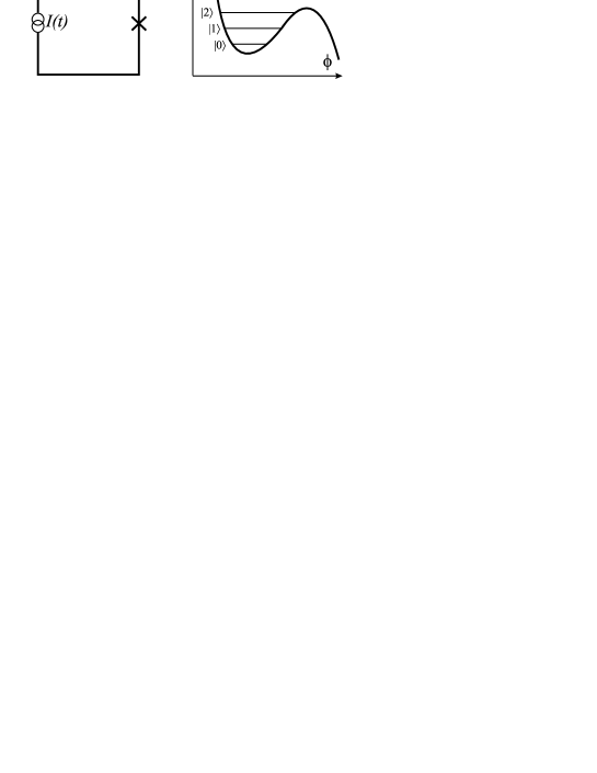
Figure 1: Phase qubit (a) and its Josephson energy (b). The metastable states $\left|0\right\rangle$ and $\left|1\right\rangle$ can be used as qubit states.

One of the effects observed in driven phase qubits is Rabi oscillations Martinis02 ; Claudon04 : coherent transitions in a quantum two-level system under the influence of a resonant perturbation, with a much lower frequency dependence on the perturbation amplitude $A$ via $\Omega_{\mathrm{R}}=\sqrt{A^{2}+\delta^{2}}$, where $\delta=\omega-\omega_{10}$ is the detuning of the driving frequency $\omega$ from the resonance frequency $\omega_{10}$. In resonance, $\Omega_{\mathrm{R}}=A$. Multiphoton Rabi oscillations, at $\omega_{10}=n\omega$ ($n$ stands for an integer), observed in such qubits Wallraff03 ; Strauch07 , were also interpreted as a signature of coherence.

The quantum coherent dynamics in phase qubits was tested by several complementary methods (see, e.g., Refs. [Martinis03, ; Claudon04, ; Strauch07, ; Lisenfeld07, ]). In particular, in Ref. [Martinis03, ] Rabi oscillations between the ground and excited state of the phase qubit were measured by applying a 25 ns pulse at $\omega_{10}$ followed by a measurement pulse at $\omega_{21}$. The probability to find the system in the upper state oscillated with the amplitude of the resonant signal, as it should in case of Rabi oscillations. In Ref. [Lisenfeld07, ] Rabi oscillations were seen instead as the resonant pulse duration varied; a dc readout was used.

However, it is known that the quantum mechanical behaviour of a quantum two-level system can still be similar to the dynamical behaviour of the classical non-linear oscillator Spreew ; Zhu ; Peano ; Wei06 ; new ; Alicki . In particular, it was recently pointed out Gr-Jen-Cir ; Marchese that due to the nonlinear behaviour of current-biased Josephson junctions, a similar effect can arise in a purely classical way. Though direct tests - à la Bell - of whether a given system is quantum or not are possible, even their simplified versions (e.g., Ref. [Alicki, ]) are demanding. This motivated us to further investigate the classical behaviour of a phase qubit and find that there is a possibility to distinguish the quantum Rabi oscillations from its classical double, by the shape of the resonance, by the fact that the classical effect can be also produced by the overtones, $n\omega_{10}$, of the resonance frequency, and by the sign of the resonant frequency shift. (An observation that a non-Lorentzian shape of the resonance should exclude a classical explanation was made already in Ref. [Berkley03, ], where the spectroscopy of two coupled qubits was performed. Also, a symmetric versus asymmetric Stark shift in a qubit playing the role of a detector was proposed to distinguish the classical and quantum behaviour of a nanomechanical oscillator Wei06 .) Classical and quantum resonances, as a function of applied drives are also studied in Ref. Savelev .

II Model

The phase qubit You-Nori ; Martinis02 is a current-biased Josephson junction. The Josephson potential, as a function of the phase difference $\phi$,

$$U_{J}(\phi)=-\frac{\hbar I_{c}}{2e}(\cos\phi+\phi I_{\mathrm{dc}}/I_{c}),$$ (1)

forms local minima, in which the quantized metastable levels serve as the working states of the qubit. Here $I_{c}$ is the critical current of the junction, and $I_{\mathrm{dc}}$ is the static bias current. A perturbation can be produced by applying a time-dependent bias current, $I_{\mathrm{ac}}\sin\omega t$. In the quantum case, the system can be reduced to a two-level model, described by the Hamiltonian Martinis03

$$\hat{H}=\frac{\Delta E}{2}\sigma_{z}+\frac{\hbar I_{\mathrm{ac}}\sin\omega t}{\sqrt{2\Delta EC}}(\sigma_{x}+\chi\sigma_{z}),$$ (2)

where $\sigma_{z,x}$ are Pauli matrices, $C$ is the capacitance of the junction, and $\chi\approx 1/4$ in the relevant range of parameters. One can obtain from here the Rabi oscillations (coherent oscillations of the probability to find the system in the upper/lower state with the frequency $\Omega_{R}$) when excited near the resonance or at its subharmonics; the shape of the resonance is a symmetric Lorentzian, as determined by, e.g., the average energy of the system versus the driving frequency $\omega$.

Unlike the flux qubit Mooij ; OSZIN , where the interlevel distance $\Delta E$ is determined by the tunneling, here $\Delta E$ is close to the “plasma” frequency $\omega_{p}=[2eI_{c}/\hbar C]^{1/2}$ of small oscillations near the local minima of the potential, Eq. (1): characteristically $\Delta E/\hbar\approx 0.95\omega_{p}$ Martinis02 . The same frequency determines the resonance in the system in the classical regime. This means that, in principle, the same AC signal could cause either the Rabi oscillations or their classical double Gr-Jen-Cir .

III Classical regime

In the classical regime, the phase qubit can be described by the RSJJ (resistively shunted Josephson junction) model Likharev ; Barone , in which the equation of motion for the superconducting phase difference across the junction, characterized by the normal (quasiparticle) resistance $R$, reads

$$\frac{\hbar C}{2e}\frac{d^{2}\phi}{dt^{2}}+\frac{\hbar}{2eR}\frac{d\phi}{dt}+I_{c}\sin\phi=I_{\mathrm{dc}}+I_{\mathrm{ac}}\sin\omega t.$$ (3)

Introducing the dimensionless variables,

$$\tau=\omega_{p}t,\text{ \ }\gamma=\omega/\omega_{p},$$ (4)

we obtain

$$\ddot{\phi}+\alpha\dot{\phi}+\sin\phi=\eta+\epsilon\sin\gamma\tau,$$ (5)

where

$$\alpha=\frac{\hbar\omega_{p}}{2eRI_{c}},\text{ }\eta=\frac{I_{\mathrm{dc}}}{I_{c}},\text{ }\epsilon=\frac{I_{\mathrm{ac}}}{I_{c}},$$ (6)

and the dot stands for the derivative with respect to $\tau$. The solution is sought in the phase-locked Ansatz,

$$\phi(\tau)=\phi_{0}+\psi(\tau),\text{ \ \ }\psi\ll 1.$$ (7)

We substitute Eq. (7) in Eq. (5) and expand $\sin\phi$ to third order, which yields

$$\ddot{\psi}+\alpha\dot{\psi}+\psi\cos\phi_{0}=\eta-\sin\phi_{0}+\frac{\sin\phi_{0}}{2}\psi^{2}+\frac{\cos\phi_{0}}{6}\psi^{3}+\epsilon\sin\gamma\tau.$$ (8)

Therefore $\sin\phi_{0}=\eta$, and introducing

$$\gamma_{0}=[1-\eta^{2}]^{1/4},$$ (9)

we obtain

$$\ddot{\psi}+\alpha\dot{\psi}+\gamma_{0}^{2}\psi=\epsilon\sin\gamma\tau+\frac{\eta}{2}\psi^{2}+\frac{\gamma_{0}^{2}}{6}\psi^{3},$$ (10)

which describes the anharmonic driven oscillator [LL, ].

Here we briefly point out several features of the solution of Eq. (10) (for more details see Chap. 5 in Ref. [LL, ]).

(i) The anharmonic driven oscillator, described by Eq. (10), is resonantly excited at any frequency $\gamma\approx\frac{p}{q}\gamma_{0}$, where $p$ and $q$ are integers. This however happens in higher approximation in the driven amplitude $\epsilon$. At small amplitude $\epsilon$ the most pronounced resonances appear at $\gamma\approx\gamma_{0}$ (main resonance), $\gamma\approx\gamma_{0}/2$ (anharmonic-type resonance), and $\gamma\approx 2\gamma_{0}$ (parametric-type resonance).

(ii) The amplitude $b$ of the small driven oscillations at the main resonance is $b_{\max}=\epsilon/(\gamma_{0}\alpha)$. When this amplitude is not small, then the phase-locked Ansatz becomes invalid. Then the solution of Eq. (5) describes the escape from the phase-locked state, which means the appearance of a non-zero average voltage on the contact. This voltage is proportional to the average derivative of the phase, $\overline{\dot{\phi}}$.

(iii) The position of the resonances for small oscillations is shifted due to the anharmonicity of the potential. This, for the main resonance $\gamma_{\mathrm{res}}$, is given by:

$$\gamma_{\mathrm{res}}-\gamma_{0} = \varkappa b^{2},$$ (11)

$$\varkappa = -\frac{3+2\eta^{2}}{48\gamma_{0}^{3}}.$$ (12)

Note that the resonance shift is negative (e.g. as in [Wei06, ]).

(iv) The shape of the resonances, as a function of the driven frequency $\gamma$, is essentially non-symmetrical. The asymmetry of the main resonance becomes pronounced at

$$\epsilon\gtrsim\frac{\gamma_{0}\alpha^{3/2}}{\left|\varkappa\right|^{1/2}},$$ (13)

at small enough damping.

(v) The parametric-type resonance at $\gamma\approx 2\gamma_{0}$ appears when the damping is sufficiently low, i.e. at

$$\alpha<\frac{\eta\epsilon}{6\gamma_{0}^{3}}.$$ (14)

At the relevant parameters, $\eta\simeq 0.9$, $\gamma_{0}\simeq 0.6$, this means the following:

$$\frac{\epsilon}{\gamma_{0}\alpha}>\frac{6\gamma_{0}^{2}}{\eta}\simeq 2,$$ (15)

which is fulfilled (see (ii)) when the solution close to the main resonance corresponds to the escape from the phase-locked state.

We note that for the anharmonic driven oscillator, described by Eq. (10), both the resonances at $\gamma_{0}/2$ and $2\gamma_{0}$ appear due to the anharmonicity of the potential energy and are of the same order. For the driven flux qubit in the classical regime OSZIN the equation for the phase variable $\theta(t)=\theta_{0}+\psi(t)$ can also be expanded for small oscillations $\psi(t)$ about the value $\theta_{0}$; restricting ourselves here to the linear in $\psi$ terms, the equation can be rewritten in the form:

$$\ddot{\psi}+\alpha\dot{\psi}+\gamma_{0}^{2}[1-h\sin\gamma\tau]\psi=\epsilon\sin\gamma\tau.$$ (16)

In this case the genuine parametric resonance at $\gamma\approx 2\gamma_{0}$ appears due to the term containing $\sin\gamma\tau\cdot\psi$ LL . This explains the prevailing of this resonance over the resonance at $\gamma\approx\gamma_{0}/2$, due to the small anharmonicity of the potential in Ref. [OSZIN, ].

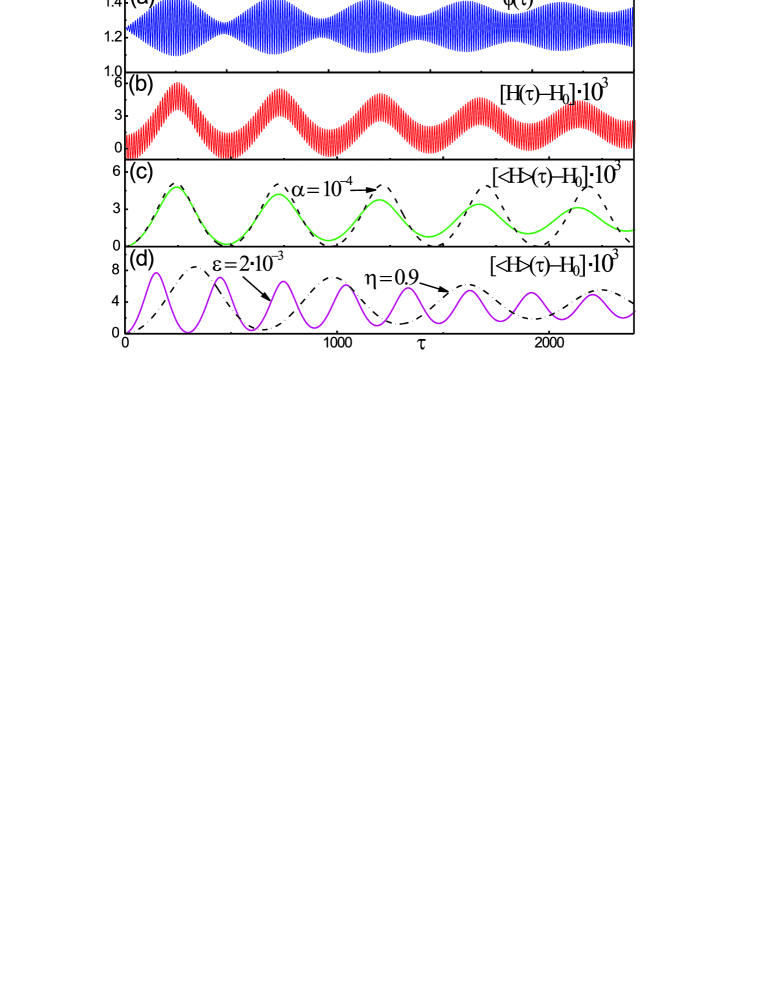
Figure 2: (Color online). Rabi-type oscillations in current-biased Josephson junctions: (a) and (b) show the time-dependence of the phase difference $\phi$ and of the energy $H$, (c) presents the time-dependence of the energy, averaged over the fast oscillations with period $2\pi/\omega$. All energies are shifted by their stationary value: $H_{0}=1-\sqrt{1-\eta^{2}}-\eta\arcsin\eta$. The parameters for the blue, red, and green curves are: $\eta=0.95$, $\alpha=10^{-3}$, $\epsilon=10^{-3}$, and $\gamma=\gamma_{0}$; for the other curves in (c) and (d) only one parameter was different from the above, for comparison. Namely: (c) dashed black line $\alpha=10^{-4}$, (d) solid violet line $\epsilon=2\cdot 10^{-3}$, dash-dotted black line $\eta=0.9$.

Now we proceed to numerically solve the equation of motion (5) for the relevant set of parameters close to the experimental case. We also investigate the behaviour of the energy of the system Likharev ; Barone

$$H=\frac{1}{2}\dot{\phi}^{2}+1-\cos\phi-(\eta+\epsilon\sin\gamma\tau)\phi,$$ (17)

which determines the thermally activated escape probability from the local minimum of the potential Gr-Jen-04 in Eq. (1). The classical Rabi-like oscillations are displayed in Fig. 2. In Fig. 2(a) the modulated transient oscillations of the phase difference $\phi$ are plotted. These oscillations result in the oscillating behaviour of the energy of the system as shown in Fig. 2(b). Averaging over fast oscillations, we plot in Fig. 2(c) with green solid curve the damped oscillations of the energy, analogous to the quantum Rabi oscillations Gr-Jen-Cir . These curves are plotted for the following set of the parameters: $\eta=0.95$, $\alpha=10^{-3}$, $\epsilon=10^{-3}$, and $\gamma=\gamma_{0}$. For comparison we also plotted the energy averaged over the fast oscillations for different parameters, changing one of these parameters and leaving the others the same. The dashed black curve in Fig. 2(c) is for the smaller damping, $\alpha=10^{-4}$; the solid (violet) line and the dash-dotted (black) line in Fig. 2(d) demonstrate the change in the frequency and the amplitude of the oscillations respectively for $\epsilon=2\cdot 10^{-3}$ and $\eta=0.9$. We notice that the effect analogous to the classical Rabi oscillations exist in a wide range of parameters.

In Fig. 3 the effect of the driving current on the time-averaged energy of the system is shown for different driving amplitudes: Fig. 3(a) for weaker amplitudes, close to the main resonance, to show the asymmetry and negative shift of the resonance; and Fig. 3(b) for stronger amplitudes, to show the resonances at $\gamma_{0}/2$ and $2\gamma_{0}$ (which are also shown closer in the insets). We note that the parametric-type resonance at $2\gamma_{0}$ originates from the third-order terms when the solution of the equation for $\psi$ is sought by iterations LL ; when there are two or more terms responsible for this resonance, the respective resonance may become splitted, which is visible in Fig. 3(b) for the lowest curve. An analogous tiny splitting of the resonance was obtained for the driven flux qubit in Fig. 4 of Ref. [OSZIN, ].

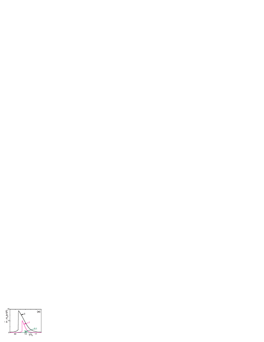
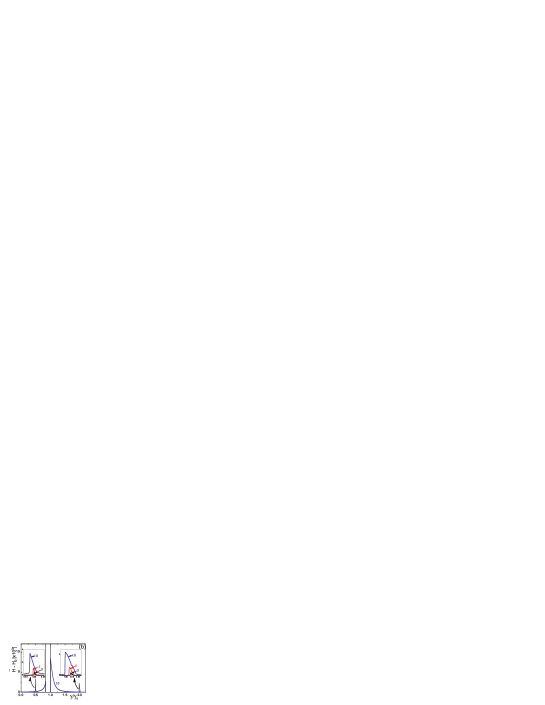
Figure 3: (Color online). The time-averaged energy $\overline{H}-H_{0}$ versus reduced frequency for relatively weak (a) and strong (b) driving. Different values of the driving amplitude $\epsilon$ (multiplied by $10^{3}$) are shown by the numbers next to the curves. The parameters are: $\eta=0.95$ and $\alpha=10^{-4}$. In (b) the region between the vertical black lines corresponds to the escape from the phase-locked state.

IV Quantum regime

In the quantum regime, the phase qubit can be described by the Bloch equations for the density matrix components. In order to take into account the relaxation and dephasing processes, the corresponding rates $\Gamma_{\mathrm{relax}}\equiv\hbar\omega_{p}\cdot\lambda_{\mathrm{relax}}$ and $\Gamma_{\phi}\equiv\hbar\omega_{p}\cdot\lambda_{\phi}$ are included in the Liouville equation phenomenologically Blum . Then the evolution of the reduced density matrix $\widehat{\rho}$, taken in the form

$$\widehat{\rho}=\frac{1}{2}\left[\begin{array}[]{cc}1+Z&X-iY\\ X+iY&1-Z\end{array}\right]\text{,}$$ (18)

is described by the Bloch equations Blum ; ShKOK :

$$\overset{\cdot}{X} =-CY-\lambda_{\phi}X,$$ (19)

$$\overset{\cdot}{Y} =-AZ+CX-\lambda_{\phi}Y,$$ (20)

$$\overset{\cdot}{Z} =AY-\lambda_{\mathrm{relax}}\left(Z-Z_{0}\right).$$ (21)

where $A$ and $C$ stand for the off-diagonal and diagonal parts of the dimensionless Hamiltonian:

$$\frac{\hat{H}}{\hbar\omega_{p}}=\frac{\Delta E}{2\hbar\omega_{p}}\sigma_{z}+\frac{\hbar I_{\mathrm{ac}}\sin\omega t}{\hbar\omega_{p}\sqrt{2\Delta EC}}(\sigma_{x}+\chi\sigma_{z})\equiv\frac{A}{2}\sigma_{x}+\frac{C}{2}\sigma_{z}.$$ (22)

From these equations we obtain $Z(\tau)$, which defines the occupation probability of the upper level,

$$P(\tau)=\rho_{22}(\tau)=\frac{1}{2}(1-Z(\tau)).$$ (23)

We choose the initial condition to be $X(0)=Y(0)=0$, $Z(0)=1$, which corresponds to the system being in the ground state; we also consider the zero-temperature limit in which the equilibrium value of $Z$ is $Z_{0}=1$.

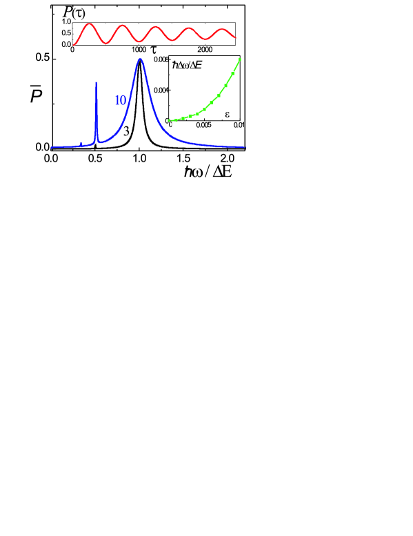
Figure 4: (Color online). The time-averaged probability $\overline{P}$ of the upper level to be occupied versus the driving frequency. The parameters used here are: $\eta=0.95$, $E_{J}/\hbar\omega_{p}=300,$ $\Gamma_{\mathrm{relax}}/\hbar\omega_{p}=\Gamma_{\phi}/\hbar\omega_{p}=3\cdot 10^{-4}$. Numbers next to the curves stand for $\epsilon$ multiplied by $10^{3}$. Upper inset: the time dependence of the probability $P(\tau)$. Right inset: the shift of the principal resonance (at $\hbar\omega\approx\Delta E$), where $\Delta\omega=\omega-\Delta E/\hbar$.

When the system is driven close to resonance, $\omega\approx\Delta E$, the upper level occupation probability $P(\tau)$ exhibits Rabi oscillations. The damped Rabi oscillations are demonstrated in the upper inset in Fig. 4, which is analogous to the classical oscillations presented in Fig. 2. After averaging the time dependent probability, we plot it versus frequency in Fig. 4 for two values of the amplitude, demonstrating the multiphoton resonances. Figure 4 demonstrates the following features of the multiphoton resonances in the quantum case: (a) in contrast to the classical case, the resonances appear only at the subharmonics, at $\hbar\omega\approx\Delta E/n$; (b) the resonances have Lorentzian shapes (as opposed to the classical asymmetric resonances); (c) with increasing the driving amplitude the resonances shift to the higher frequencies – the Bloch-Siegert shift, which has the opposite sign from its classical counterpart. The Bloch-Siegert shift (the shift of the principal resonance at $\hbar\omega\approx\Delta E$) is plotted numerically in the right inset in Fig. 4. Analogous shifts of the positions of the resonances were recently observed experimentally Strauch07 .

V Conclusions

In conclusion, the following criteria can be proposed to distinguish classical Rabi-type oscillations in current-biased Josephson junctions: (1) the appearance of resonances both at the overtones of the main resonant frequency (e.g., $2\gamma_{0}$) and its subharmonic ($\gamma_{0}/2$); (2) the asymmetric shape of the resonances; (3) a negative shift of the resonant frequency when increasing the driving amplitude. In recent publications these features were not reported: the multiphoton resonances were observed Wallraff03 ; Strauch07 ; the resonances observed have a Lorentzian shape Berkley03 ; Claudon04 ; comment and have a positive frequency shift Strauch07 , which means that the observed resonant excitations in the system were in the quantum regime.

- (1) You J Q and Nori F 2005 Physics Today 58, No. 11, 42
- (2) Martinis J, Nam S, Aumentado J and Urbina C 2002 Phys. Rev. Lett. 89 117901
- (3) Claudon J, Balestro F, Hekking F W J and Buisson O 2004 Phys. Rev. Lett. 93 187003
- (4) Wallraff A, Duty T, Lukashenko A and Ustinov A V 2003 Phys. Rev. Lett. 90 037003
- (5) Strauch F W, Dutta S K, Paik H, Palomaki T A, Mitra K, Cooper B K, Lewis R M, Anderson J R, Dragt A J, Lobb C J and Wellstood F C 2007 IEEE Trans. Appl. Supercond. 17 105
- (6) Martinis J M, Nam S, Aumentado J, Lang K M and Urbina C 2003 Phys. Rev. B 67 094510
- (7) Lisenfeld J, Lukashenko A, Ansmann M, Martinis J M and Ustinov A V 2007 Phys. Rev. Lett. 99 170504
- (8) Spreeuw R J C, van Druten N J, Beijersbergen M W, Eliel E R and Woerdman J P 1990 Phys. Rev. Lett. 65 2642
- (9) Zhu Y, Gauthier D J, Morin S E, Wu Q, Carmichael H J and Mossberg T W 1990 Phys. Rev. Lett. 64 2499
- (10) Peano V and Thorwart M 2004 Phys. Rev. B 70 235401
- (11) Wei L F, Liu Y X, Sun C P and Nori F 2006 Phys. Rev. Lett. 97 237201
- (12) Rotoli G, Bauch T, Lindstrom T, Stornaiuolo D, Tafuri F and Lombardi F 2007 Phys. Rev. B 75 144501
- (13) Alicki R and Van Ryn N 2008 J. Phys. A 41 062001
- (14) Grønbech-Jensen N and Cirillo M 2005 Phys. Rev. Lett. 95 067001
- (15) Marchese J E, Cirillo M and Grønbech-Jensen N 2007 Open Systems and Information Dynamics 14 189
- (16) Berkley A J, Xu H, Ramos R C, Gubrud M A, Strauch F W, Johnson P R, Anderson J R, Dragt A J, Lobb C J and Wellstood F C 2003 Science 300 1548
- (17) Savel’ev S, Hu X and Nori F 2006 New J. Phys. 8 105; Savel’ev S, Rakhmanov A L, Hu X, Kasumov A and Nori F 2007 Phys. Rev. B 75 165417
- (18) Mooij J E, Orlando T P, Levitov L, Tian L, van der Wal C H and Lloyd S 1999 Science 285 1036
- (19) Omelyanchouk A N, Shevchenko S N, Zagoskin A M, Il’ichev E and Nori F arXiv:0705.1768
- (20) Likharev K 1986 Dynamics of Josephson Junctions and Circuits (New York: Gordon and Breach)
- (21) Barone A and Paterno G 1982 Physics and Applications of the Josephson Effect (New York: Wiley-Interscience)
- (22) Landau L D and Lifshitz E M 1976 Mechanics (Oxford: Pergamon)
- (23) Grønbech-Jensen N, Castellano M G, Chiarello F, Cirillo M, Cosmelli C, Merlo V, Russo R and Torrioli G 2006 in “Quantum Computing in Solid State Systems”, eds. Ruggiero B, Delsing P, Granata C, Pashkin Y and Silvestrini P p.111 (Springer)
- (24) Blum K 1981 Density Matrix Theory and Applications (New York–London: Plenum Press)
- (25) Shevchenko S N, Kiyko A S, Omelyanchouk A N and Krech W 2005 Low Temp. Phys. 31 564
- (26) We note passing by that in other types of qubits also the Lorentzian-shaped multiphoton resonances were observed nak01 ; yaponci ; Oliver ; multiphoton ; Sillanpaa
- (27) Nakamura Y, Pashkin Yu A and Tsai J S 2001 Phys. Rev. Lett. 87 246601
- (28) Saito S, Thorwart M, Tanaka H, Ueda M, Nakano H, Semba K and Takayanagi H 2004 Phys. Rev. Lett. 93 037001
- (29) Oliver W D, Yu Ya, Lee J C, Berggren K K, Levitov L S and Orlando T P 2005 Science 310 1653
- (30) Shnyrkov V I, Wagner Th, Born D, Shevchenko S N, Krech W, Omelyanchouk A N, Il’ichev E and Meyer H-G 2006 Phys. Rev. B 73 024506
- (31) Sillanpää M, Lehtinen T, Paila A, Makhlin Yu and Hakonen P 2007 J. Low Temp. Phys. 146 253; 2006 Phys. Rev. Lett. 96 187002