Probing the submillimetre number counts at $f_{850{\rm\mu m}}<2$ mJy

Abstract

We have conducted a submillimetre mapping survey of faint, gravitationally lensed sources, where we have targeted twelve galaxy clusters and additionally the NTT Deep Field. The total area surveyed is 71.5 arcmin² in the image plane; correcting for gravitational lensing, the total area surveyed is 40 arcmin² in the source plane for a typical source redshift $z\approx$ 2.5. In the deepest maps, an image plane depth of 1$\sigma$ r.m.s. $\sim$ 0.8 mJy is reached. This survey is the largest survey to date to reach such depths. In total 59 sources were detected, including three multiply-imaged sources. The gravitational lensing makes it possible to detect sources with flux density below the blank field confusion limit. The lensing corrected fluxes ranges from 0.11 mJy to 19 mJy. After correcting for multiplicity there are 10 sources with fluxes $<2$ mJy of which 7 have sub-mJy fluxes, doubling the number of such sources known. Number counts are determined below the confusion limit. At 1 mJy the integrated number count is $\sim$ 10⁴ deg^-2, and at 0.5 mJy it is $\sim$ 2$\times$10⁴ deg^-2. Based on the number counts, at a source plan flux limit of 0.1 mJy, essentially all of the 850 $\mu$m background emission has been resolved. The dominant contribution ($>50$ per cent) to the integrated background arises from sources with fluxes $S_{\it 850}$ between 0.4 and 2.5 mJy, while the bright sources $S_{850}>$ 6 mJy contribute only 10 per cent.

1 Introduction

The first submillimetre mapping instrument SCUBA (Submillimetre Common User Bolometer Array; Holland et al., 1999), which is mounted at the James Clerk Maxwell Telescope (JCMT) at Hawaii, allowed for observations of IR luminous galaxies at high redshift. The first observations at 850 $\mu$m (Smail et al., 1997) showed that these objects are much more common at earlier epochs. Subsequently, a number of surveys have been undertaken to study this population of submm detected galaxies. The blank field surveys include observations of the Hubble Deep Field North (HDF-N) (Hughes et al., 1998; Borys et al., 2003; Serjeant et al., 2003), the Hawaii Deep Fields (Barger et al., 1999), Canada-UK Deep SCUBA Survey (CUDSS) (Eales et al., 2000; Webb et al., 2003), the 8 mJy survey (Scott et al., 2002), Galactic regions (Barnard et al., 2004), the Groth strip (Coppin et al., 2005), the SHADES survey (Coppin et al., 2006), and a re-analysis of several blank field surveys (Scott et al., 2006). In particular CUDSS and SHADES have been successful in covering a large area of the sky. However, the blank field surveys are limited by the confusion at 2 mJy at 850 $\mu$m with the 15 m JCMT and hence do not probe the number counts of the fainter population. The submillimetre extragalactic background light (Fixsen et al., 1998; Puget et al., 1996) is, however, dominated by the population around 1 mJy (e.g. Barger et al., 1999; Blain et al., 1999; Cowie et al., 2002). To break the blank field confusion limit observing with SCUBA, gravitational lensing must be employed. The UK-SCUBA Lens Survey (Smail et al., 1997, 2002) targeted seven galaxy cluster fields. Three of their fields were observed to larger depth (Cowie et al., 2002). Another lens survey was performed by Chapman et al. (2002), however, this survey was relatively shallow.

Submillimetre observations of objects at high redshifts, $z>1$, benefit from the fact that the geometrical dimming of the light is cancelled by the negative $k$-correction, resulting from the fact that the peak of the spectral energy distribution (SED) is shifted toward the observing band. For a given luminosity, the observed submm flux is close to constant between redshift 1 and 8. Consequently, extragalactic submm observations primarily probe the high redshift universe. Furthermore, deeper surveys do not probe deeper into the universe, but only sample lower luminosity galaxies. Galaxies in clusters at redshifts $z<1$ are not expected to be seen with SCUBA, except for sometimes the central cD galaxy (Edge et al., 1999) or an Active Galactic Nucleus (AGN).

We here present the Leiden-SCUBA Lens Survey, in which we have targeted twelve galaxy clusters. This is the largest survey so far of gravitationally lensing clusters, and it is the first survey to substantially probe below the blank field confusion limit. This paper presents the observations, the analysis of the data, the resulting catalogue and the number counts. The analysis involves the mathematically rigorous Mexican Hat wavelets algorithm (e.g. Cayón et al., 2000) and Monte Carlo simulations. In following papers, we will use the derived number counts as an observational constraint on models of the submm galaxy population, and we will present multiwavelength follow-up observations.

In Section 2 we present the observations and the reduction of the data. The source extraction is discussed in detail in Section 3. The issue of confusion is discussed in Section 4, and the effect of gravitational lensing is discussed in Section 5. The resulting catalogue is presented in Section 6. Finally, in Section 7 we present the number counts for the survey. Throughout the paper we assume $\Omega_{m}=0.3$, $\Omega_{\Lambda}=0.7$ and $H_{0}=70\,{\rm km/s/Mpc}$.

2 Observations and reduction

We have obtained observations of a number of clusters of galaxies at 850 $\mu$m and 450 $\mu$m with SCUBA. In addition we have obtained similar observations of the NTT Deep Field (Arnouts et al., 1999), which was chosen due to the large, deep data set existing at optical and near-infrared wavelengths. In total our survey contains twelve fields of galaxy clusters and the one blank field covering an area of 71.5 arcmin². The parameters for each field are listed in Table 1.

Table 1: The observed fields.

Name	RA(J2000)			Dec(J2000)			$z_{cl}$	$t_{int}$	$\Omega_{850}$	$\sigma_{deep}^{850}$	$\sigma_{wghtd}^{850}$	$\sigma_{deep}^{450}$	$\sigma_{wghtd}^{450}$
	h	m	s	∘	′	′′		hours	arcmin2	mJy/$\Omega_{b}$	mJy/$\Omega_{b}$	mJy/$\Omega_{b}$	mJy/$\Omega_{b}$
Cl0016+16(⋆)	00	18	33.2	$+$16	26	17.8	0.541	7.73(5.46)	4.5	1.33	2.00	9.8	16.5
A478(⋆)	04	13	25.3	$+$10	27	54.3	0.0881	7.08	4.3	1.59	2.05	9.1	14.5
A496	04	33	37.8	$-$13	15	43.0	0.0328	10.4	4.1	1.08	1.47	11.6	17.2
A520	04	54	07.0	$+$02	55	12.0	0.202	19.6(18.0)	4.3	0.97	1.26	9.2	14.5
MS1054$-$03	10	56	56.1	$-$03	36	26.0	0.826	49.2	14.4	0.86	1.49	3.7	10.2
A1689(⋆)	13	11	17.0	$-$01	20	29.0	0.181	33.4(32.2)	5.4	0.70	0.97	4.4	9.9
RXJ1347.5$-$1145(⋆)	13	47	30.5	$-$11	45	09.0	0.451	10.5	4.8	2.04	3.06	7.2	24.8
MS1358+62	13	59	50.6	$+$62	31	05.1	0.328	4.80	4.2	1.39	1.81	7.6	11.2
A2204⋆	16	32	46.9	$+$05	34	33.0	0.1523	1.60	4.0	3.75	5.20	65.3	87.2
A2218	16	35	54.2	$+$66	12	37.0	0.171	42.3(35.6)	7.7	0.65	1.06	3.2	16.0
A2219(⋆)	16	40	20.4	$+$46	42	59.0	0.225	9.63	4.6	1.10	1.54	6.7	11.8
A2597	23	25	19.8	$-$12	07	26.4	0.0852	6.76	4.1	1.34	1.77	11.2	17.8
NTT Deep Field	12	05	22.6	$-$07	44	14.9	–na–	27.1	5.0	0.78	0.97	3.9	6.3

SCUBA has two arrays of 37 and 91 bolometers optimized for 850 $\mu$m respectively 450 $\mu$m. A dichroic beamsplitter is used for simultaneous observations with both arrays. Both arrays have the bolometers arranged in a hexagonal pattern. Because SCUBA does not have a field rotator, the arrays appear as rotating on the sky. The field–of–view on the sky, which is approximately the same for both arrays, is roughly circular with a diameter of 2.3’. The observations were carried out in jiggle mode with a 64 point jiggle pattern, in order to fully sample the beam at both operating wavelengths. Subtraction of the strong sky background was done through 7.8 Hz chopping with the secondary mirror. Our observations were performed with a chop throw of 45^′′ with the chopping position angle fixed in right ascension (RA). As a result the beam pattern has a central positive peak with negative sidelobes on each side, each with minus half the peak value, a pattern which can be used for the detection of at least the brighter sources. During the observations the pointing was checked every hour by observing bright blazars near the targeted fields. The noise level of the arrays was checked at least twice during an observing shift, and the atmospheric opacity, $\tau$, was determined with JCMT at 850 $\mu$m and 450 $\mu$m every two–three hours and supplemented with the $\tau_{225{\rm GHz}}$ data from the neighboring Caltech Submillimetre Observatory (CSO). Calibrators were observed every two to three hours. If available, primary calibrators, i.e. planets, preferably Uranus, were observed at least once during an observing shift. Our observations were supplemented with archival SCUBA data, hence the data set includes twelve cluster fields and the NTT Deep Field.

The data were reduced using the surf package (Jenness & Lightfoot, 1998). First the chop of the secondary mirror was removed, i.e. the off–source measurements were subtracted from the on–source measurements. Then the varying responses of the bolometers were corrected by dividing with the array’s flatfield. The extinction correction was performed based on the atmospheric opacity measured both with the JCMT and CSO. The $\tau_{850\mu{\rm m}}$ and $\tau_{450\mu{\rm m}}$ was measured a number of times during the night with the JCMT. As the atmospheric opacity may change on shorter timescales, the interpolated $\tau$-values may be somewhat inaccurate. At the CSO on the other hand, the opacity is measured every few minutes at 225 GHz. Using the linear relations between $\tau_{225{\rm GHz}}$ and $\tau_{850\mu{\rm m}}$ respectively $\tau_{450\mu{\rm m}}$, deduced by Archibald et al. (2000), it is possible to determine the atmospheric opacity at the time of the observations. The zenith opacity was for most of the time 0.12 $<\tau_{850\mu{\rm m}}<$ 0.40. The data were inspected for bad or useless data. For each scan for each bolometer datapoints deviating by more than three sigma, based on the r.m.s. of the individual bolometer, were rejected from further analysis. This statistical exclusion is possible because there are no bright sources present in the data. Furthermore, the data were inspected by eye, and bolometers that were clearly more noisy than other bolometers were flagged and excluded from further analysis. The pointing of each scan was corrected using the pointing observations taken just before and after the observations. The r.m.s. pointing error of the JCMT is typically 2^′′. The correlated atmospheric fluctuations still present in the data were subtracted using the pixel–by–pixel median of the 25 least noisy bolometers.

Data taken after January 2002, were affected by a periodic noise of currently unknown origin. This was first pointed out by (Borys et al., 2004), and has later been discussed by Webb et al. (2005), Sawicki & Webb (2005), and Coppin et al. (2006). For these data, the power spectrum of the individual bolometers showed that some bolometers had a spike around 1/16s. This spike, however, did not systematically occur in the same bolometers or with the same strength. This effect was corrected for by performing a sky subtraction based on the bolometers that were not affected by this, and additionally, the affected bolometers were corrected through multiple-linear regression (T. Webb, private communication). As only a small fraction of the data for the survey was obtained after January 2002, this is relevant mostly for the MS1054-03 data, where the data most affected was the Northern pointing. The correction for the 1/16s spike brought down the noise in the affected data by $\sim$ 10 per cent.

The scans were calibrated by multiplying by the flux conversion factors (FCF) determined from the calibration maps. The FCFs are determined from the peak values (or the values corrected for extendedness) of the used calibrators. We estimate the uncertainty in the flux calibration as approximately 10 per cent at 850 $\mu$m. At 450 $\mu$m, the calibration uncertainty is about 30 per cent, because of variations in the beam profile resulting from thermal deformations of the dish. This is in agreement with the canonical calibration uncertainties. The data were despiked by projecting the data on a grid and at each map pixel rejecting the associated bolometer pixels deviating by more than three sigma. Finally, all the bolometers were weighted based on their measured r.m.s. noise relative to one another and to the whole data set. The data were regridded with 1^′′ pixels into a final map. The beam sizes are $\sim$ 14.3^′′ at 850 $\mu$m respectively $\sim$ 7.5^′′ at 450 $\mu$m. The noisy edge was trimmed by removing the outer 23 pixels; 23 pixels corresponds to one and a half beam. Unless otherwise mentioned the maps used in the analysis have been smoothed with a 5^′′ full width half maximum (FWHM) Gaussian to reduce high spatial frequency noise, resulting in beam sizes of 15.1^′′ at 850 $\mu$m and 9^′′ at 450 $\mu$m.

3 Source extraction

The sensitivity in the reduced maps is not uniform across the field. As we are working close to the signal–to–noise limit of these data it is crucial to understand the properties of the noise. Furthermore, the source extraction from maps like the SCUBA maps is a non–trivial task, which must be performed with a robust and well–understood method. In a previous paper (Knudsen et al., 2006), we describe the approach, which we adopt for this survey and first applied to the data for the field A2218. In summary, the noise is measured across a map using Monte Carlo simulations, where the real data (i.e. the time streams) are substituted by the output from a random number generator with a Gaussian distribution and the same statistical properties as the real data. The simulated data is reduced following the same procedure as the real data, creating empty maps, and the standard deviation is measured for each pixel using about 500 simulated maps. Furthermore, in order to remove the chopping pattern (caused by the motion of the secondary mirror) from the beam we use the CLEAN algorithm (Högbom, 1974). For details, see Knudsen et al. (2006).

3.1 Point source detection

Most sources at high redshifts have an angular extent on the sky of less than a few arcseconds. In the 850 $\mu$m beam such sources will appear as point sources. To do the point source extraction we choose to use Mexican Hat Wavelets (MHW). MHW is a mathematically rigorous tool for which the performance can be fully understood and quantified. MHW has proven to be a powerful source extraction technique in both SCUBA jiggle-maps and scan-maps (Barnard et al., 2004; Knudsen et al., 2006). Wavelets are mathematical functions used for analysing according to scale. Isotropic wavelets have the advantage that no assumptions about the underlying field need to be made. The beam at 850 $\mu$m is well-described by a 2-dimensional Gaussian, which is best detected with the ’Mexican Hat’ wavelets; the ’Mexican Hat’ is the second derivative of a Gaussian. The software utilized are programmes written for the anticipated Planck Surveyor mission, but modified for application on SCUBA maps. For more details and the application of the programmes on SCUBA maps see Cayón et al. (2000); Barnard et al. (2004); Knudsen et al. (2006). Here we summarize only the relevant details.

The MHW source extraction is done in the following way. Point source candidates are selected at positions with wavelet coefficient values larger than a given number. For each candidate, the wavelet function is compared to the theoretical variations expected with the scale, as a further check on the source’s shape. A $\chi^{2}$ value is calculated between the expected and the experimental results. If the $\chi^{2}$ is smaller than a given limit, i.e., the region surrounding the identified peak has the characteristics of a Gaussian point source of the correct dimensions, the point source is included in the extracted catalogue. In Knudsen et al. (2006) we have performed controlled detection experiments to determine the optimal criteria for the MHW algorithm applied to SCUBA jiggle maps: the wavelet coefficient $\geq 2$ and $\chi^{2}\leq 4$. These we combine with the $S/N\geq 3$ criterion in the flux map.

In doing the source extraction, the MHW algorithm searches the maps for features at the scale of the beam, features with scales smaller or larger than the beam are not extracted. E.g., in the field RX J1347.5$-$1145 the extended emission presumably due to the Sunyaev-Zel’dovich effect (Komatsu et al., 1999) is undetected by MHW point source detection. Also extended sources cannot be detected by changing the $\chi^{2}$-limit. This of course ensures that all sources detected are point sources.

To check for undetected sources located closer than one beam to a detected source, the detected sources are subtracted from the map. If those are the only point sources present in the map, then MHW finds no sources in the residual map. If any sources are significantly detected in the residual map, those sources are subtracted from the original map and a new MHW detection is done in order to improve the result on the first detection. This is continued iteratively until the output converges. This approach does not resolve extended sources.

As described in Knudsen et al. (2006), we performed detection experiments doing Monte Carlo simulations to analyse and determine the accuracy of the derived parameters (position and flux). In the simulations point sources are added on to empty maps and recovered using the MHW algorithm. We perform this for all fields and find similar results. The accuracies derived through this are included in the final errors quoted in Table 3.

3.2 Completeness

The completeness was determined through a similar set of simulations as those mentioned above, where point sources are added on to empty maps and recovered using the MHW algorithm with the same constraints as for the real data. This is done for each field, for a representative range of fluxes in steps of 1-2 mJy, repeated 4000 times for each flux level. The positions were chosen to be random with a uniform distribution. As the simulations are performed on the whole field, which has a non-uniform sensitivity, the results we find is an average across each field. In Figure 1 we plot the completeness for the individual fields. As is seen in Figure 1, the completeness depends on the depth of the observations. For the deepest fields like A1689, A2218 and NTT Deep Field the observations are 80 per cent complete at a flux level of $\sim$ 3.5-4 mJy and 50 per cent at $\sim$ 2.6-2.8 mJy. For the other, less deep fields the 80 per cent completeness is 4.5-7.5 mJy and 50 per cent at 3.5-5.5 mJy. For A2204, which is a shallow field, the observations are 80 per cent complete at 18 mJy and 50 per cent at 14 mJy.

Figure 1: This figure shows the completeness as function of flux for all the surveyed fields. For a better overview the thirteen fields have been plotted in the three panels. The top panel shows the deepest of the fields, while the middle panel shows the medium-deep fields, and the lower panel shows two medium-deep fields, and shallower fields. Note that the x-axis is different for each panel.

3.3 Spurious detections

We have addressed the issue of spurious sources. Source detection was performed on inverted maps to check if any negative sources were detected. We ignore negative sources sitting on a chop throw, which are a known artifacts from the original beam pattern. Furthermore, we ignore the deepest fields, where confusion plays a role. For those fields even a detected negative source can be a real structure in the background. Along the edges many negative sources were detected. As this indicates that many positive spurious sources would be found along the edge, we have decided to trim away the edge at a width of one and a half beam, i.e. 23^′′. In total we find five negative sources, which is in agreement with Gaussian statistics. Our catalogue thus may contain 5 spurious sources.

Additionally, we have performed source extraction from the Monte Carlo maps (see above) for all the fields. We find that in a hundred maps typically two sources were detected with $S/N\approx$ 3, and no sources with $S/N>$ 3.5. This demonstrates the reliability of MHW to pick out real sources with $S/N>$ 3. With essentially no sources in the pure noise maps, the spurious sources detected in the inverted maps are probably due to the structured background.

Coppin et al. (2006) used a Bayesian approach to flag potential spurious soures. In the method, which is described in detail in Coppin et al. (2005), an a priori probability distribution is folded with the detection to calculate a posterior probability distribution, $P(S_{j})$, for each individual source. We adopt this approach and the prior is found determined from simulations of the submm sky assuming the number counts from (Coppin et al., 2006) and using the beam-pattern as known for the individual fields. We flag the sources, which have a more than 5 per cent of their posterior probability distribution below 0 mJy, $P(S_{j}<0\,{\rm mJy})>5$ per cent. These sources will be marked in the catalogue table (Table 3). The total number of sources is 11. The sources are not removed from the catalogue, as this is only a statistical approach and does not allow us to discriminate unambigiously between real and spurious sources as is evidenced in the field MS1054-03.

3.4 The 450 $\mu$m maps

The atmospheric optical depth at 450 $\mu$m is five times larger than that at 850 $\mu$m. This makes it difficult to reliably calibrate the 450 $\mu$m maps, as the data are much more sensitive to any variation in the sky opacity. As opposed to the 850 $\mu$m beam pattern, the 450 $\mu$m beam pattern is not well-described by a 2-dimensional Gaussian. In addition, the 450 $\mu$m beam pattern is very sensitive to any deformation of the JCMT dish. Such deformations are normally the result of temperature variations. Consequently, the beam pattern changes during the night, with changing observing conditions. These effects complicate a reliable source extraction from the 450 $\mu$m. Furthermore, the 450 $\mu$m beam is much narrower than the 850 $\mu$m beam, and more of the calibration sources may appear extended. This has to be taken into account as well and might add to the uncertainty of the 450 $\mu$m flux calibration.

We have chosen not to perform deconvolution and MHW source extraction from the 450 $\mu$m maps to make a separate 450 $\mu$m point source catalogue. Instead we use the maps to determine the 450 $\mu$m flux at the 850 $\mu$m source positions. That is done in the following way. The $S/N$ map, the flux and the noisemap are used. In a circle with radius 4^′′ around the 850 $\mu$m source position, the maximum $S/N$ value is found. If this value is equal to or greater than 3, the flux value in that pixel is adopted as the $S_{450}$ of the 850 $\mu$m source, and the uncertainty, $\sigma_{S_{450}}$, is 30 per cent of that value. If no pixels in that circle fullfil the $S/N$ criteria, an upper limit is given as three times the mean flux value corresponding to the three lowest noise values within the circle. This has been done three times for all the 450 $\mu$m maps, namely when the maps have been smoothed with a Gaussian with FWHM of 5^′′, 10^′′ and 12.7^′′. Smoothing with e.g. a 5^′′ Gaussian reduces the high spatial frequency noise, while smoothing with a 12.7^′′ Gaussian makes the 450 $\mu$m beam equivalent to the 850 $\mu$m beam. Furthermore, the smoothing reduces the effect that sources might be slightly extended in the original map due to intrinsic size and pointing errors. In a couple of cases the $S/N$ criterion is met with one smoothing, but not quite in the other one(s). For the reasons described above, the 450 $\mu$m fluxes listed in Table 3 should used with caution.

4 Confusion

4.1 Confusion limit in blank fields

In the background of deep SCUBA maps the instrumental noise and the confusion noise from a fainter submm population are of approximately equal magnitude. We adopt the formalism of Condon (1974) and use the same definition for the beam as Hogg (2001): $\Omega_{beam}=\pi(\theta_{FWHM}/2.35)^{2}$, where $\theta_{FWHM}$ is the width of the beam (SCUBA at 850 $\mu$m: $\theta_{FWHM}=$ 15^′′). We adopt the rule of thumb that the number of sources per beam should not exceed one source per 30 beams before the image is considered confused (e.g., Hogg, 2001). The confusion limit is the flux, $S_{conf}$, at which the number of sources in the map is one source per 30 beams. To estimate the confusion limit, the integrated number counts, $N(>\!S)$, where $N(>\!S)$ denotes the number density on the sky of sources brighter than $S$, are used. For blank fields a single power law suffices to describe the number counts, $N(>S)=N_{0}S^{-\alpha}$. For $N(>S)=1/30\Omega_{beam}$, the confusion limit is $S_{conf}=\sqrt[\alpha]{30\Omega_{beam}N_{0}}$. If we assume $\alpha=$ 2.0 and $N_{0}=$ 13000 deg^-2 (based on e.g., Barger et al., 1999; Borys et al., 2003), for SCUBA 850 $\mu$m blank field observations, the confusion limit is $\sim$ 2 mJy. For an average-sized, trimmed map in our survey of 5 arcmin², this number of sources is $n_{s}=$ 4.7. This is close to the average number of sources per field in our survey.

Confusion in the maps affects the position and flux determination. Hogg (2001) have made general simulations addressing the issue of the errors caused by confusion. Based on Figure 4 of his paper (Hogg, 2001), which gives the position error as function of detected source density where no prior knowledge is used in the source detection, in the Euclidean case, a detected source density of one per 30 beams causes a median position error of 0.25 times the half width at half maximum (HWHM). At 850 $\mu$m this corresponds to an additional error in the position of 1.9^′′. For crowded fields in our survey where the source density is larger than one per 30 beams, the error in the position caused by the confusion is 4-5^′′. Eales et al. (2000) found in their simulations that in confusion-limited fields 10 per cent to 20 per cent of the detected sources would lie outside an error circle of 6^′′. Furthermore, they found that the fluxes of the sources were boosted by a median factor of 1.44, albeit with a large scatter. However, as argued by Blain (2001), confusion effects will only appear in SCUBA maps with detection limits of 2 mJy or less at 850 $\mu$m; hence most of our data are relatively unaffected by flux boosting, though flux boosting is expected to play a role in the deepest maps, i.e. A1689, A2218, NDF and possibly A520. For these fields we adopt the Bayesian approach as used by Coppin et al. (2005, 2006), and as already mentioned in Subsect. 3.3, to estimate how large the flux boosting might be. The estimated de-boosted flux is listed in the catalogue Table 3. The deboosted fluxes are about 1 mJy fainter, though the actual number is connected with the $S/N$ of the detection.

4.2 Confusion limit in lensed fields

For the cluster fields the confusion limit is affected by the gravitational lensing. The gravitational lensing magnifies the region seen behind the cluster, hence the source plane is smaller than the image plane. The number of beams is conserved between the image plane and the source plane, i.e. the size of the beam scales with the magnification. This is why it is at all possible to observe the fainter sources, which have a higher surface density than the brighter sources.

The number counts in the lensed case can be written as $N_{lens}=(N_{0}/\mu)(S/\mu)^{-\alpha}$ $=N_{blank}\mu^{\alpha-1}$, where $\mu$ is the gravitational lensing magnification. The confusion limit in the lensed case can thus be written as $S_{conf}=\sqrt[\alpha]{30\Omega_{beam}N_{0}\mu^{1-\alpha}}$. As the lensing magnification varies across the field, We use the average magnification for a field as estimated by the ratio of the area in the image plane and the area in the source plane. This simple estimate gives an average across the field, which in some cases means that the estimated lensed confusion limit does not reflect the confusion limit of the highly magnified region close to the caustics. For the most extreme case in our sample, A1689, where the source plane area surveyed is 20 times smaller than the SCUBA field of view, the confusion limit is reduced by a factor 4.5, i.e., $S_{conf}=$ 0.44 mJy. The confusion limits for the cluster fields based on this simple calculation are given in Table 2. In the simplified estimate of the confusion limit presented here we assumed that the number counts are described by a single power law. There are good indications that the number counts are described by a double power law or another function with a (gradual) turn-over (see Sect. 7). Including this in such a calculation will work in a favourable direction and the confusion limit in the source plane will be lower.

5 Gravitational lensing

To quantify the gravitational lensing effect we use LENSTOOL (Kneib et al., 1993).

Figure 2: Histogram showing the distribution of the magnification factors. The histogram is binned with $\Delta\mu=$ 1, except between 1 and 2, where the bin-size is 0.5.

The gravitational potential of each galaxy cluster is mapped in a mass model, which describes the distribution of the overall potential of the cluster and to some extent of the individual galaxies. For clusters where the cluster lensing is a less strong effect only the brightest cluster galaxies are considered in the mass model in addition to the global cluster potential. For clusters where the cluster lensing is a dominant effect many galaxies have been included to map the substructure of the total potential, as individual galaxies might cause extra lensing of the background sources. The lensing correction is done for the individual submm sources and for the sensitivity maps. The latter are needed in the calculation of the number counts.

Figure 3: The area as function of magnification for the individual fields. This has been split into two figures for clarity. The top panel shows the fields with a relatively less strong lensing effect, while the bottom panel shows those with a stronger lensing effect. We have assumed a source redshift of $z=$ 2.5. Placing the source plane at a different redshift, $z>$ 1, would not make a significant difference.

As the redshift is not yet known for a majority of the objects, we assume $z=2.5$ for the objects with unknown redshift based on the redshift distribution from Chapman et al. (2003, 2005). Likewise, the sensitivity maps, which give us the observational sensitivity in the image plane, are traced to a source plane at $z=$ 2.5. The actual redshift distribution of the faint SMGs is not known and it is also not known whether it follows that of the brighter SMGs as deduced by Chapman et al. (2005). Based on a stacking analysis, (Wang et al.2006) suggest that the redshift distribution of faint SMGs peaks at redshifts of one or less. However, in Knudsen et al. (2005) submm stacking results of high redshift red galaxies show that half of the EBL light produced by at the faint end originates from red galaxies in the redshift interval 1-4. Of the five $f_{850}<1$ mJy SMGs with reliable identification and spectroscopic redshifts, the redshifts are z = 1.0, 2.5, 2.5, 2.6 and 2.9 (Kneib et al., 2004; Borys et al., 2004; Knudsen et al., 2006, and see appendix for A1689), showing no evidence for a radically different distribution than the one deduced by Chapman et al. (2005). We note that not knowing the exact redshifts of the SMGs will introduce some uncertainty in the lensing correction, however, the magnification correction is only weakly dependent on redshift at $z>1$, where we expect most of the sources to be.

The magnification factors of the individual sources range from 1.1 to 23. We have plotted a histogram of the magnification factors in Fig. 2. About 40 per cent of the sources are magnified by factors $\mu\,>$ 2, while 20 per cent are magnified by 1.5 $<\,\mu\,<$ 2, and 40 per cent have relatively low magnification factors 1 $<\,\mu\,<$ 1.5. We have plotted the area as function of magnification factor for the individual fields in Figure 3, and the area as function of source plane sensitivity for the whole survey Figure 4. In Figure 3, the two most extreme cases are A1689, where the area surveyed is a factor 20 smaller in the source plane than in the image plane, and MS1054-03, where the average over the large angular area surveyed of the cluster dilutes the strong lensing effect caused by the core of the cluster. The total area observed by our survey in these 13 fields is 71.5 arcmin². When taking into account the gravitational magnification the area of the cluster fields is reduced to 35 arcmin² in the source plane. The area of the individual fields as well as the sensitivity in the source plane is listed Table 2. For comparison the seven cluster fields from the UK-SCUBA Lens Survey are 40 arcmin² in the image plane and 15 arcmin² in the source plane (Smail et al., 2002). Likewise, in the deep though small survey by (Cowie et al., 2002), the area in the image plane is 18 arcmin²; assuming a reasonable amplification this corresponds to 6 arcmin² in the source plane.

Figure 4: The area as function of 1$\sigma$ sensitivity for the whole survey. The dashed line represents the area in the image plane, and the solid line represents the area in a source plane at redshift $z=$ 2.5. The actual area surveyed in the source plane is a factor two smaller than what we observe in the field of view of SCUBA at 850 $\mu$m. For the twelve cluster fields the total area of useful data in the image plane is 66.5 arcmin² and in a source plane at redshift $z=$ 2.5 is 35 arcmin².

The uncertainties of the corrected fluxes and positions introduced by the lensing are in most cases small. The magnification is generally a monotonic function of the redshift (except in the very central part of a strong lensing cluster), but for source redshifts twice larger than the lens redshift, the amplification is only weakly increasing with redshift. As essentially all the SCUBA sources are expected to be at $z>$1, redshift dependence in the lensing correction is only a minor effect. However, the position of the source relative to the cluster centre and cluster members can play an important role, as the magnification can vary from $\sim$ 2 to $\sim$ 20 for typical background sources. The uncertainty in the magnification (assuming a known redshift) is directly linked to the uncertainty in the mass model. The closer the object is to a critical line, the higher its magnification will be and the larger the uncertainty on the magnification will be. At most four of the SCUBA sources lie relatively close to critical lines and therefore their magnification factors are subject to larger uncertainties. However, on an ensemble basis, when e.g. deriving the counts in terms of unlensed flux, the error in magnification is compensated by the error in lensed area, thus the change in the unlensed counts due to uncertainty in the mass model is of the second order.

We estimate the uncertainty of the magnification factors of the individual sources through a Monte Carlo simulation. The magnification is determined at 1600 positions with a normal distribution within the $1\sigma$ error circle centered on the MHW position. In Table 3 we give the median magnification from the MC simulations together with the 68 per cent deviation of the magnifications determined at the MC positions. For very large magnification factors, typically $>10$, such as seen for the multiple-imaged galaxies in A1689, which are close to the caustics, the MC magnification factor distribution has both a large skewness and kurtosis. While we have made an estimate of the strength of possible flux-boosting, the results of these MC simulations show that the uncertainties on the magnification factor often exceeds the flux-boosting.

Identification of multiply-imaged galaxies in the sample is important, as a repeated counting of the same source will affect the number counts. In total three multiply-imaged sources are found in the fields of the strongly lensing clusters A1689 and A2218. The galaxy in A2218 is triple-imaged with a total magnification factor of 45 and has been studied extensively (Kneib et al., 2004; Sheth et al., 2004; Kneib et al., 2005; Garrett et al., 2005). The two other galaxies are present in A1689, one is triple-imaged and the other is a quintuple-imaged galaxy, both with spectroscopic redshift $\sim 2.5$. Their identification will be discussed in a future paper.

Table 2: The area in the source plane at redshift $z=$ 2.5, an estimate of the source plane confusion limit (also see subsection 4.2), and the area-weighted 1$\sigma$ sensitivity in the source plane.

Cluster	$\Omega_{s.pl.}$	$S_{conf}$	$\sigma_{wghtd}^{850}$
	arcmin2	mJy	mJy
Cl0016+16	3.1	1.7	1.48
A478	3.3	1.7	1.65
A496	2.7	1.6	0.98
A520	2.2	1.4	0.78
MS1054$-$03	11.9	1.8	1.17
A1689	0.3	0.4	0.13
RXJ1347.5$-$1145	1.2	1.0	1.06
MS1358+62	2.0	1.3	1.17
A2204	1.3	1.1	2.23
A2218	2.9	1.2	0.50
A2219	2.3	1.4	1.06
A2597	1.7	1.3	0.78

6 The catalogue

In the twelve cluster fields we detect 54 sources and in the NTT Deep Field we detect 5 sources. The sources have been named according to their detection (SMM) and their J2000 coordinates. The catalogue of the extracted point sources is given in Table 3. After correcting for lensing multiplicity, we have detected 15 sources below the blank field confusion limit. Of these, 7 have flux densities $<$ 1 mJy, which doubles the number of known sub-mJy sources (compare Cowie et al. 2002, Smail et al. 2002 and Borys et al. 2004). A description of the individual fields can be found in Appendix A along with the final maps.

Table 3: Catalogue of source positions, submm fluxes and uncertainties. $S$ is the flux, $S/N$ is the signal-to-noise of the detection in flux units, the $\sigma$’s give the uncertainties in the flux and position. The uncertainties do not take into account possible additional uncertainties due to confusion. For the position, the additional confusion-uncertainty is $\sim$ 1.9^′′ (as described in Section 4). The ^⋆ after the source name indicates that the source has a $P(S_{j}<0\,{\rm mJy})>5\%$ (as described in subsection 3.3). $\mu$ is the lensing magnification, while $\mu_{\rm MC}$ is the lensing magnification from Monte Carlo simulations (see Section 5). $S_{850}$(deboost) is the deboosted flux (see subsection 4.1).

name	$\sigma_{pos}$	$S_{850}$	$S/N$	$\sigma_{S_{850}}$	$S_{450}$	$S/N_{450}$	$\sigma_{S_{450}}$	$z$	$\mu$	$\mu_{\rm MC}$	$S_{850}$(deboost)
	′′	mJy		mJy	mJy		mJy				mJy
Cl0016+16
SMM J001828.9$+$162617⋆	4.0	6.5	3.2	2.2	$<34.2$	…	…	2.5	1.2	$1.2\pm 0.02$
SMM J001829.4$+$162653⋆	4.0	5.8	3.2	2.0	$<77.9$	…	…	2.5	1.2	$1.2\pm 0.02$
SMM J001834.2$+$162517	4.0	7.0	3.9	2.4	$<56.1$	…	…	2.5	1.3	$1.3\pm 0.03$
SMM J001835.1$+$162559⋆	4.0	5.3	3.1	1.8	$<34.2$	…	…	2.5	2.0	$2.0^{+0.3}_{-0.2}$
A478
SMM J041322.9$+$102806⋆	3.8	6.8	3.3	2.5	$<35.3$	…	…	2.5	1.2	$1.2\pm 0.02$
SMM J041323.4$+$102657	3.1	7.9	4.2	2.1	$<53.9$	…	…	2.5	1.3	$1.3\pm 0.02$
SMM J041327.2$+$102743	2.3	25.0	14.4	2.8	55.4	5.3	16.6	2.837	1.3	$1.3\pm 0.03$
SMM J041328.7$+$102805⋆	3.8	9.0	3.8	3.3	$<32.8$	…	…	2.5	1.3	$1.3\pm 0.02$
A496
SMM J043334.7$-$131526⋆	4.1	4.7	3.1	1.7	$<43.6$	…	…	2.5	1.4	$1.4\pm 0.03$
SMM J043335.4$-$131454⋆	4.1	5.3	3.3	1.9	$<54.7$	…	…	2.5	1.4	$1.4\pm 0.02$
SMM J043336.5$-$131547	3.2	4.8	4.0	1.7	51.1	3.0	15.3	0.03	…	…
SMM J043337.4$-$131558	4.1	4.7	3.8	1.7	$<42.9$	…	…	0.03	…	…
SMM J043337.6$-$131627	3.0	9.0	5.5	1.6	$<40.3$	…	…	2.5	1.5	$1.5\pm 0.03$
SMM J043337.8$-$131541	3.0	7.9	5.7	1.4	$<39.4$	…	…	0.03	…	…
SMM J043338.9$-$131444	4.1	4.0	3.1	1.4	$<67.3$	…	…	2.5	1.4	$1.5\pm 0.04$
SMM J043339.4$-$131637	4.1	4.8	3.6	1.7	$<52.1$	…	…	2.5	1.4	$1.4\pm 0.02$
SMM J043340.1$-$131533	3.0	6.4	5.1	1.1	$<36.9$	…	…	2.5	1.5	$1.5\pm 0.04$
A520
SMM J045403.1$+$025547	3.3	4.7	4.1	1.1	$<31.9$	…	…	2.5	1.5	$1.5\pm 0.03$	$3.7\pm 1.3$
SMM J045406.2$+$025410⋆	4.2	3.9	3.1	1.4	$<32.6$	…	…	2.5	5.5	$5.5\pm 0.4$	$3.4\pm 1.3$
SMM J045406.7$+$025435⋆	4.2	4.3	3.1	1.5	$<37.0$	…	…	2.5	4.5	$4.4^{+0.6}_{-0.4}$	$2.3\pm 1.6$
SMM J045409.7$+$025510	3.3	6.0	4.4	1.4	29.0	2.7	8.7	2.5	1.7	$1.7\pm 0.05$	$4.7\pm 1.5$
MS1054$-$03
SMM J105649.3$-$033606	3.3	5.0	3.6	1.1	$<17.6$	…	…	2.5	1.1	$1.07\pm 0.003$
SMM J105655.8$-$033610	3.3	3.9	3.8	0.9	25.6	3.4	7.7	2.5	1.1	$1.11\pm 0.007$
SMM J105656.3$-$033635	3.3	3.9	3.7	0.9	$<21.2$	…	…	2.5	1.1	$1.18\pm 0.01$
SMM J105657.0$-$033612	2.8	4.9	4.8	0.9	61.7	3.6	18.5	2.5	1.1	$1.12\pm 0.008$
SMM J105700.3$-$033513	3.9	3.5	3.2	1.1	$<20.2$	…	…	2.5	1.1	$1.05\pm 0.003$
SMM J105700.3$-$033544	3.3	4.4	3.5	1.0	28.1	3.6	8.4	2.5	1.1	$1.08\pm 0.004$
SMM J105701.8$-$033827	3.3	4.7	3.5	1.1	$<27.9$	…	…	2.5	1.3	$1.3\pm 0.03$
SMM J105702.2$-$033604⋆	3.9	4.4	3.0	1.4	$<21.8$	…	…	2.423	1.1	$1.11\pm 0.007$
SMM J105703.7$-$033730	3.9	4.2	3.3	1.4	62.7	5.7	18.8	2.5	1.6	$1.6\pm 0.05$

Table 3: — Continued from previous page.

name	$\sigma_{pos}$	$S_{850}$	$S/N$	$\sigma_{S_{850}}$	$S_{450}$	$S/N_{450}$	$\sigma_{S_{450}}$	$z$	$\mu$	$\mu_{\rm MC}$	$S_{850}$(deboost)
	′′	mJy		mJy	mJy		mJy
A1689
SMM J131125.7$-$012117	3.3	5.0	3.9	1.6	$<66.4$	…	…	2.5	3.9	$3.9\pm 0.4$	$3.7\pm 1.5$
SMM J131128.6$-$012036	4.3	2.6	3.4	0.8	…	…	…	2.5	23.6	$17.6^{+28.4}_{-10.6}$	$1.9\pm 0.9$
SMM J131128.8$-$012138	4.3	3.6	3.3	1.2	$<32.9$	…	…	2.5	5.8	$6.5^{+3.9}_{-1.0}$	$2.4\pm 1.1$
SMM J131129.1$-$012049	2.8	4.7	6.0	0.8	21.4	4.4	6.4	2.5	21.6	$18.7^{+19.1}_{-6.6}$	$4.3\pm 0.8$
SMM J131129.8$-$012037	4.3	2.5	3.2	0.8	$<11.3$	…	…	2.5	3.3	$3.1\pm 1.3$	$1.7\pm 0.9$
SMM J131132.0$-$011955	3.3	3.3	3.6	1.0	$<14.8$	…	…	2.5	9.7	$8.6^{+6.9}_{-1.5}$	$2.4\pm 1.1$
SMM J131134.1$-$012021	3.3	3.2	4.0	1.0	$<12.4$	…	…	2.5	6.5	$6.5^{+1.1}_{-0.8}$	$2.6\pm 0.9$
SMM J131135.1$-$012018	3.3	4.9	4.2	1.6	$<17.6$	…	…	2.5	3.8	$3.9\pm 0.5$	$3.9\pm 1.3$
RX J1347.5$-$1145
SMM J134728.0$-$114556	3.0	15.5	5.7	3.1	98.7	12.8	29.6	2.5	3.0	$3.0\pm 0.3$
MS1358+62
SMM J135957.1$+$623114	3.2	6.7	4.4	1.3	$<25.5$	…	…	2.5	1.5	$1.5\pm 0.08$
A2204
SMM J163244.7$+$053452	3.2	22.2	4.9	5.7	$<219.5$	…	…	2.5	3.4	$3.4^{+0.5}_{-0.4}$
A2218
SMM J163541.2$+$661144	2.6	10.4	7.5	1.4	53.4	3.5	16.0	2.5	1.7	$1.7\pm 0.07$	$9.5\pm 1.4$
SMM J163550.9$+$661207	2.4	8.7	11.5	1.1	22.9	5.9	6.9	2.515	9.0		$8.4\pm 0.8$
SMM J163554.2$+$661225	2.3	16.1	21.7	1.6	46.4	12.4	13.9	2.515	22		$15.9\pm 0.7$
SMM J163555.2$+$661238	2.2	12.8	16.9	1.5	31.8	8.3	9.5	2.515	14		$12.5\pm 0.8$
SMM J163555.2$+$661150	3.3	3.1	3.8	0.7	17.1	4.7	5.1	1.034	7.6	$7.1^{+13.0}_{-2.8}$	$2.4\pm 0.9$
SMM J163555.5$+$661300	2.2	11.3	15.8	1.3	$<11.8$	…	…	2.5	3.4	$4.2^{+1.0}_{-0.8}$	$11.1\pm 0.7$
SMM J163602.6$+$661255	3.3	2.8	3.5	0.6	$<14.5$	…	…	2.5	1.8	$1.8\pm 0.08$	$2.1\pm 0.9$
SMM J163605.6$+$661259	3.1	5.2	4.9	0.9	$<17.4$	…	…	2.5	1.5	$1.5\pm 0.03$	$4.4\pm 1.1$
SMM J163606.5$+$661234	3.1	4.8	4.6	0.8	$<17.4$	…	…	2.5	1.6	$1.7\pm 0.01$	$4.0\pm 1.1$
A2219
SMM J164019.5$+$464358	2.9	10.0	5.8	2.0	53.4	5.0	16.0	2.5	1.2	$1.2\pm 0.02$
SMM J164025.5$+$464255⋆	3.7	5.1	3.1	1.7	29.4	2.9	8.8	2.5	1.5	$1.5\pm 0.1$
A2597
SMM J232519.8$-$120727	2.6	12.3	7.1	1.8	$<37.9$	…	…	0.08	…	…
SMM J232523.4$-$120745	4.1	5.2	3.2	1.7	71.2	5.0	21.4	2.5	2.1	$2.1\pm 0.1$
NTT Deep Field
SMM J120519.0$-$074409	3.3	3.8	4.0	0.9	$<16.0$	…	…				$3.0\pm 1.1$
SMM J120520.6$-$074448	4.0	3.0	3.2	0.8	$<13.7$	…	…				$2.0\pm 1.1$
SMM J120522.1$-$074431	3.3	3.5	3.9	0.9	$<14.0$	…	…				$2.7\pm 1.0$
SMM J120523.1$-$074516	4.0	3.4	3.4	0.9	$<16.7$	…	…				$2.3\pm 1.2$
SMM J120525.1$-$074512	3.3	4.0	4.3	0.9	$<23.8$	…	…				$3.3\pm 1.0$

7 Number counts

7.1 Determining the number counts from maps of non-uniform sensitivity

The notation $N(>S)$ is typically used for cumulative number counts: the number of sources per unit solid angle brighter than a flux limit $S$. Calculating the cumulative number counts by counting the number of sources with $>S$ must be done on a map with uniform sensitivity. SCUBA maps, however, do not have uniform sensitivity. The problem of determining number counts for maps of non-uniform sensitivity has previously been discussed for several of the blank field surveys (Webb et al., 2003; Borys et al., 2003; Coppin et al., 2006; Scott et al., 2006). The presence of gravitational lensing results in even larger non-uniformity compared to some of the large blank field surveys and complicates any completeness corrections. We here present the number counts as deduced using two different approaches. In both cases cluster members like cD galaxies are excluded and also the sources, which we have marked as potentially spurious using the scheme from Coppin et al. (2005) (see subsection 3.3). Taking into account that the multiply-imaged sources each count as one, the total number sources in the number counts analysis is 40.

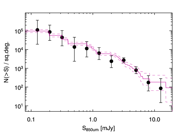
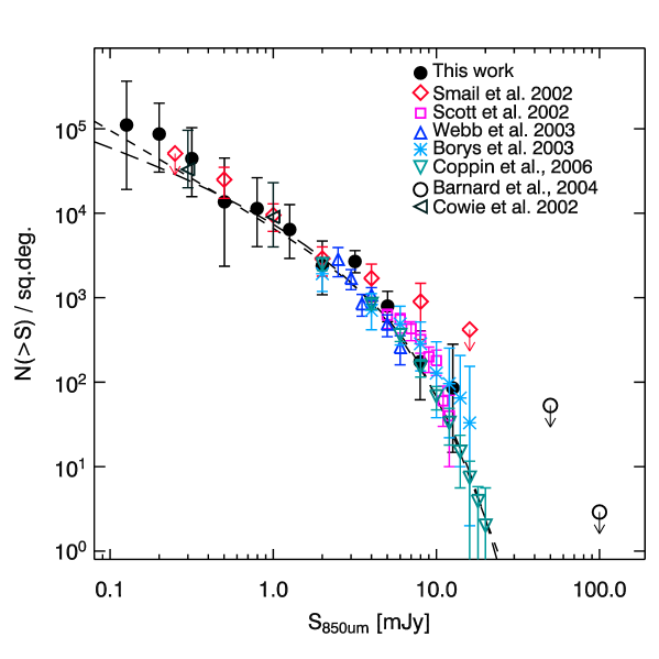
Figure 5: The 850 $\mu$m number counts, $N(>\,S)$, as determined from this work. The number counts are determined based on the data from 12 cluster fields and one blank field. The data from the cluster fields have first been corrected for the gravitational lensing. Seven sources have been detected with sub-mJy fluxes. This doubles the number of such sources known (compare Cowie et al., 2002). Upper panel:  The black dots show the results from the first approach for determining the number counts and the solid (magenta) line bracketed by the dashed show the results of the second approach (for details see text). Lower panel: The number counts from other fields have been plotted together with the number counts from this work. The short dashed line shows the best-fit double powerlaw, Eq. 3, and the long dashed line shows the best-fit Schechter function, Eq. 4.

The first approach: For a given flux level $S$, only the surveyed area where 3$\sigma<S$ is considered. The $N(>S)$ is then the number of sources with $>S$ within that area divided by the source plane area, $\Omega_{<S}$. For the cluster fields we use the fluxes and sensitivity maps corrected for the gravitational lensing, as described in the previous section. Upper and lower errors are calculated using Poisson statistics weighted by the area, $\Omega_{<S}$. We use the tables for confidence limits on small numbers of events from Gehrels (1986). It should be noted that at each $S$ only a small number of sources is counted, in particular at the faint and bright end, as is reflected in the error bars. The resulting number counts for the 850 $\mu$m observations are plotted in Figure 5. The number counts, $N(>S)$, the number of sources for each data point and the area, $\Omega_{<S}$, are given in Table 4. Due to the non-uniform sensitivity across the observed fields, the area $\Omega_{<S}$ varies with $S$. Consequently, $N(>S)$ is not uniformly decreasing with $S$, which would otherwise be expected for cumulative number counts determined in fields with uniform sensitivity. We note that even though the area of the circle with diameter 15^′′ is 0.049 arcmin², and that the counts for $S_{850}<$ 0.2 are calculated from an area that appears to be smaller than the beam in the image plane, it should be remembered that the area is in the source plane, which due to the large magnification would appear as a much larger area in the image plane corresponding to many beams.

We use a second, alternative approach to estimate the number counts:

$$N(>S)=\int^{\infty}_{S}\frac{n(S^{\prime})}{\Omega_{eff}}\mathrm{d}S^{\prime}\ ,$$ (1)

where $n(S^{\prime})$ is the number density of sources within the flux interval $S^{\prime}$ and $S^{\prime}+\mathrm{d}S^{\prime}$. $\Omega_{eff}$ is the effective area over which the survey is sensitive to sources with flux $>S$ is given by

$$\Omega_{eff}=\Omega_{total}\cdot C(S)\ .$$ (2)

$\Omega_{total}$ is the total area of the survey. $C(S)$ is the completeness function, that also takes into account the effects of the lensing, which is determined through simulations as follows. Sources are placed at random in the source plane and run through the lensing models (Sect. 5) to determine their magnification. This is done for each flux level $S$ and compared with the sensitivity map to determine how large a fraction of the simulated sources would be detectable. For the sources from the deepest fields we use their deboosted fluxes. Similarly to above, the upper and lower errors are calculated using Poisson statistics weighted by the area and use the tables for confidence limits on small numbers of events from Gehrels (1986). This approach allows us to take into account the deboosted fluxes of the deepest maps. The results are also plotted in Figure 5. As opposed to the previous approach, the error bars are very small at the faint fluxes due the larger total number of sources. We caution that these error bars do not contain systematic errors caused by e.g. uncertainties in the lensing correction.

The number counts are probed to the faintest source in the survey, which has a lensing corrected flux of 0.11 mJy. The faint end of the number counts is dominated by the two cluster fields A1689 and A2218, which on the other hand do not contribute much at the bright end. A tentative analysis of the number counts show that the counts are not well-described by a single power-law function, but are better described by a double power-law

$$\frac{{\rm d}N(>S)}{{\rm d}S}=\frac{N_{0}}{S_{0}}\bigg{(}\bigg{(}\frac{S}{S_{0}}\bigg{)}^{\alpha}+\bigg{(}\frac{S}{S_{0}}\bigg{)}^{\beta}\bigg{)}^{-1}\ ,$$ (3)

or another function with a turn-over, such as a Schechter function

$$\frac{{\rm d}N(>S)}{{\rm d}S}=\frac{N_{0}}{S_{0}}S\bigg{(}\frac{S}{S_{0}}\bigg{)}^{\alpha}\exp\bigg{(}\frac{-S}{S_{0}}\bigg{)}\ .$$ (4)

We have performed a simple $\chi^{2}$-analysis for these two functions, as these two have been used previously for numerical modeling or analysis of SCUBA number counts. For this we have also included the number counts from the SHADES survey (Coppin et al., 2006) as these provide a better constraint at the brighter end. We have also included the additional constraint that the integrated light well below 0.1 mJy should not be larger the extragalactic background light (Puget et al., 1996; Fixsen et al., 1998). We note that the slope at the faint end is diverging and if it was to continue to much fainter fluxes it would result in an overproduction of the background light. The resulting parameters from this analysis are given in Table 5 as well as the best fit is overplotted on top of the number counts shown in Figure 5.

Table 4: The 850 $\mu$m number counts.

$S_{850}$	$N(>S)$	Nsrc	$\Omega_{<3\sigma}$
mJy	arcmin-2		arcmin2
0.13	$30.8_{-25.4}^{+70.7}$	1	0.033
0.20	$24.1_{-15.5}^{+31.8}$	2	0.083
0.32	$12.3_{-7.96}^{+16.3}$	2	0.16
0.50	$3.88_{-3.13}^{+8.71}$	1	0.26
0.80	$3.15_{-2.04}^{+4.16}$	2	0.63
1.26	$1.78_{-0.97}^{+1.73}$	3	1.69
2.00	$0.66_{-0.36}^{+0.64}$	3	4.54
3.17	$0.75_{-0.20}^{+0.26}$	14	18.8
5.02	$0.22_{-0.076}^{+0.11}$	8	36.2
7.96	$0.049_{-0.031}^{+0.064}$	2	41.2
12.6	$0.024_{-0.020}^{+0.054}$	1	42.2

Table 5: The resulting parameters from fits to the 850 $\mu$m number counts.

Function	$N_{0}$	$S_{0}$	$\alpha$	$\beta$
Eq. 3	$658\pm 48$	$9.60^{+0.30}_{-2.12}$	$2.12^{+0.14}_{-0.08}$	$6.22^{+0.51}_{-0.34}$
Eq. 4	$1039\pm 69$	$4.30\pm 0.08$	$-2.62\pm 0.10$	…

7.2 Fluctuation analysis

We have performed a fluctuation analysis, or $P(D)$ analysis, on the NDF, A1689 and A2218 fields. This has previously been done for blank field (sub)mm data by Hughes et al. (1998) and (Maloney et al.2005) as a statistical method to probe the number counts fainter than the sensitivity limit of the data. We measure the pixel distribution from simulated maps, which were created using an input source distribution, convolved with the beam and added to the Monte Carlo maps from Section 3. As number counts for the input source distribution we used the Schechter function, Eq. 4, stepping through the three different parameters. The positions of the simulated sources were drawn from a set of random positions with a normal distribution without taking into account clustering. For the A1689 and the A2218, we calculated the effects of the gravitational lensing of the simulated sources, i.e. the magnification and position in the image plane. We caution that gravitational lensing will introduce similar uncertainties and effects as when calculating the lensing effects for the real sources and hence adding an extra complication for the interpretation of the results. The $P(D)$ of the simulated data is compared to that of the real data for the three fields to determine the parameter set of the number counts that best fit the real data. The resulting parameters are listed in Table 6 along with some calculated counts values for comparison with the number counts determined in the previous subsection. As seen for both the NDF and A1689, $\alpha<-3.5$, gives a very steep function especially at the faint end which would strongly overproduce the EBL. The resulting parameters from A2218 are reasonably close to those deduced the Schechter function fit to the number counts.

Table 6: Results from the fluctuation analysis.

Field	$N_{0}$	$S_{0}$	$\alpha$	$N(>2$mJy$)$	$N(>1$mJy$)$	$N(>0.5$mJy$)$	$N(>0.2$mJy$)$
NDF	550	4.0	-3.75	1750 deg-2	8700 deg-2	…	…
				0.49 arcmin-2	2.4 arcmin-2	…	…
A1689	650	4.0	-3.5	…	…	24600 deg-2	114600 deg-2
				…	…	6.8 arcmin-2	31.8 arcmin-2
A2218	750	6.5	-2.75	…	…	30700 deg-2	72400 deg-2
				…	…	8.5 arcmin-2	20.1 arcmin-2

We note that although all fields are roughly equally deep in the image plane, the faint counts are best probed by A2218, since NDF is not gravitationally lensed so that that field does not probe faint fluxes very well, and A1689 covers only a very small area in the source plane. As $P(D)$ analysis is a statistical tool it is best applied on large fields as was done by e.g.  (Maloney et al.2005).

7.3 Comparison with other surveys

Here we will compare the derived number counts with those determined through other surveys, both lensed surveys and blank field surveys. The number counts from other studies have been plotted together with the number counts from this work in Figure 5.

Lensing surveys: Three other studies of SCUBA observations of cluster fields have been published: For the UK-SCUBA Lens Survey seven cluster fields were targeted and number counts were determined to $S_{850}=$ 0.5 mJy (e.g., Smail et al., 1997; Blain et al., 1999; Smail et al., 2002). Cowie et al. (2002) obtained deeper SCUBA observations of three of these fields. A shallower cluster survey was performed by (Chapman et al., 2002), in which eight clusters were observed with SCUBA, however, no sub-mJy sources were detected. For $>1$ mJy, our number counts agree with those of (Chapman et al., 2002). Here we will focus the comparison on the surveys from Cowie et al. (2002) and Smail et al. (2002). As both those surveys are relatively small in area, a comparison is only interesting where such surveys have their strength, namely at the faint fluxes. Cowie et al. (2002) detect five sub-mJy sources. We detect seven sub-mJy sources, and thereby double the number of known sub-mJy sources. Our faint number counts are in good agreement with those of Cowie et al. and Smail et al.

Blank field surveys: Blank field surveys are surveys with no strongly gravitationally lensing clusters present in the surveyed area. Such surveys typically cover much large areas than the lensed surveys, and are limited in depth by the blank field confusion limit ($\sim$ 2.0 mJy). Hence the strength of those surveys lies at brighter fluxes. Several such surveys have been carried out: The Canada-UK Deep SCUBA Survey (CUDSS) (Eales et al., 2000; Webb et al., 2003), covered 75 arcmin² to the blank field confusion limit. The 8mJy-survey (Scott et al.) covered an area of 260 arcmin² to a flux limit $>$ 5 mJy/beam. The Hubble Deep Field North (HDF-N) has been surveyed extensively, which has been brought together in the so-called “HDF-N SCUBA supermap” by Borys et al. (2003), which covers 165 arcmin² to depths between 0.4 and 6 mJy/beam. Barger et al. (1999) have surveyed the Hawaii Survey Fields covering an area of 104 arcmin² to a flux limit of 8 mJy with a small area of 7.7 arcmin² almost to the confusion limit. Coppin et al. (2005) surveyed 70 arcmin² of the Groth Strip to a depth of $1\sigma$ rms. $\approx 3.5$ mJy. A re-analysis of several blank field surveys was carried out by Scott et al. (2006). Finally the results of the SHADES survey were published by Coppin et al. (2006), where 720 arcmin² were covered to a noise level of $\sim 2$ mJy uncovering more than a 100 submillimetre galaxies. Through a detailed analysis Coppin et al. (2006) determine the first differential submm number counts and fit their results with a double power law. With minor deviations, there is an overall good agreement between the bright end the number counts of the work presented here and previous work. Though, we do find that the slope of the power-law at the bright end is a bit steeper than previous work ($\alpha\sim$ 1.9-2.2).

7.4 Resolving the extragalactic submillimetre background light

Using the differential number counts from equation 3, we calculate the integrated background light. At $S\sim$ 0.10 mJy, the integrated background produced by our sources is comparable to the background light detected with COBE (Puget et al., 1996; Fixsen et al., 1998). Given that sources with fluxes below 0.1 mJy also contribute to the integrated background, there is a possibility that our counts overpredict the integrated background somewhat. The overproduction of the background light, which is caused by the shape of the number counts at the faint end, is possibly due to the low number statistics. Given the differential counts from equation 3 the dominant contribution to the integrated background light comes from the sources with fluxes $S_{850}$ between 0.4 mJy and 2.5 mJy with 50 per cent of the background resolved at 1 mJy. The latter is in agreement with the results from Smail et al. (2002), Cowie et al. (2002) and Chapman et al. (2002). Sources with $S_{850}>$ 2.5 mJy contribute $\sim$ 25 per cent to the integrated background, of which sources with $S_{850}>S_{0}$ contribute only $\sim$ 10 per cent. This means that the bulk of the submm energy output from the submm galaxy population arises from sources just fainter than the blank field confusion limit.

8 Conclusions

We have conducted a deep submm survey using SCUBA. We have observed twelve clusters of galaxies and the NTT Deep Field. The total area surveyed is 71.5 arcmin² in the image plane. For the cluster fields the total area in the source plane is 35 arcmin². This is the largest deep submm lens survey of its type to date. The gravitational  lensing  reduces  the  confusion  limit  allowing for observations of  sources with $S_{850}<$ 2 mJy. The data have been analysed using Monte Carlo simulations to quantify the noise properties, Mexican Hat Wavelets have been used for source extraction and simulations were performed to quantify the error of the analysis.

• In total 59 sources have been detected, of which 10 have flux densities below the blank field confusion limit. Four are associated to cluster cD galaxies. Three sources in the field of A2218 are multiple images of the same galaxy, and in A1689 five are associated with two multiply-imaged galaxies.

• The number of sub-mJy sources is seven, which doubles the number of such sources.

• The integrated number counts are probed over two decades in flux down to 0.10 mJy. The number counts cannot be described by a single power law, but have to be described by a double power law or another function with a turn-over. Describing the differential counts by a double power law function we find that the turn-over is $\sim$ 6 mJy. At 1 mJy the number counts are $\sim$ 10⁴ deg^-2 and at 0.5 mJy they are $\sim$ 2$\times$10⁴ deg^-2, based on derived differential counts.

• Another key result is that essentially all of the integrated submm background is resolved. At 1 mJy 50 per cent of the background is resolved, and at 0.4 mJy 75 per cent is resolved. The dominant contribution to the background comes from sources with fluxes $S_{850}$ between 0.4 mJy and 2.5 mJy, while the bright sources with fluxes $S_{850}>$ 6 mJy contribute only 10 per cent. This means that the bulk of the energy comes from submm galaxies with fluxes just below the blank field confusion limit.

The submm number count distribution is an observable for the submm galaxy population as a whole and provides strong constraints on the models describing the submm galaxy population and their evolution. While the submm number counts are well studied at the bright end ($>2$ mJy), the faint end ($<2$ mJy) and the extremely bright end ($>20$ mJy) remain difficult to probe. The extremely bright end is challenged by the steep counts. The faint end is challenged by the blank field confusion limit. The present survey has made a substantial contribution to the faint end, however, it essential to follow this through with future instrumentation such as more sensitive instruments like SCUBA-2 and LABOCA, with which an even larger number number of strongly lensing clusters can be surveyed, larger telescopes such as the LMT and CCAT for which the blank field confusion limit will be lower, and of course ALMA which will be able to study the faint sources in great detail.

Appendix A Description of the individual fields

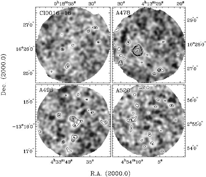
Figure 6: The signal-to-noise ($S/N$) 850 $\mu$m SCUBA maps of the clusters Cl0016+16, A478, A496 and A520. The overlayed contours represent $S/N=$ 3,4,5,6,7, but for A478 the contours represent $S/N=$ 3,4,5,6,8,10,12,14. The stars $\star$ indicate the position of the detected sources.

Cl0016+16  In this field, four point sources were detected with $3<S/N<4$. The magnification factors for the four sources are between 1.2 and 2.2. The corrected fluxes of the sources are between 2.4 and 5.2 mJy. We note that three sources have more than 5 per cent of their posterior probability distribution below 0 mJy. None of the sources have significant 450 $\mu$m flux detections. A shallower SCUBA map of this field is presented in Chapman et al. (2002), where the depths is about a factor two shallower than our map. Within the positional uncertainties the two sources from Chapman et al. are coincident with SMM J001834.2+162517 and SMM J001835.1+162559, though we find that the observed fluxes are fainter than in Chapman et al. The mass model is based on the results from Natarajan (private communication) with a substantially more detailed description compared to that of Chapman et al.

A478   This cluster is well-known in cooling-flow studies (e.g., White et al., 1991). Some of the SCUBA data presented here were obtained by others to study the cooling-flow, however, the cooling-flow has not been detected in the data. Four point sources are detected. With a detected flux of $S_{850}=$ 25$\pm$3 mJy the source SMM J041327.2+102743 is the brightest source in the survey. This source has been studied in detail and is identified with a type-1 quasar at redshift $z=$ 2.837 (Knudsen et al., 2003, there denoted SMM J04135+10277). The three fainter sources have $S/N$ between 3.3 and 4.2. All four sources have magnification factors of 1.2-1.3. The fluxes of the three other sources are 5.6-7.3 mJy. We note that two sources have more than 5 per cent of their posterior probability distribution below 0 mJy. The quasar is the only source in this field with 450 $\mu$m flux detection. Close to the SE-edge a fifth bright source is detected, however, as it is less than 1.5 beam from the edge it is not included in the catalogue. The mass model is a simple model, which we constructed based on the published velocity dispersions: the model includes the cluster potential and the potential of the cD galaxy (Zabludoff et al., 1990; Allen et al., 1993).

A496   This is the lowest redshift cluster in the survey. Nine point sources have been detected. Even though this cluster has not been observed to the blank field confusion limit, the large number of sources might introduce extra uncertainties on the derived parameters. Three sources towards the centre of the field are just 14^′′ (just smaller than a beam) from one another. One of the central sources, SMM J043337.8$-$131541, is coincident with the cD. The two other central sources, SMM J043337.4$-$131558 and SMM J043336.5$-$131547, are so close (just less than a beam) to the centre of the cD galaxy, that they are likely associated with cD galaxy. The latter of those two sources has a probable detection of 450 $\mu$m emission. All three central sources will be excluded from the further analysis in this paper. In Figure 6, source SMM J043338.9$-$131444 has no $S/N=$ 3 contour as it is located in a depression in the background. The six sources not associated with the central cD galaxy are magnified by factors 1.3-1.4 and have unlensed fluxes of 3-6.3 mJy. We note that two sources have more than 5 per cent of their posterior probability distribution below 0 mJy. This large number of sources in a low-z cluster field is surprising. Follow-up observations indicate that they are not cluster members, which might otherwise be expected because of the low redshift of the cluster. Like A478, the lens mass model is a simple model including the cluster potential and the cD galaxy (Peletier et al., 1990; Zabludoff et al., 1990).

A520   The optical centre and the X-ray centre of A520 is not coincident, and the cluster seems to be undergoing strong dynamical evolution, as the cD galaxy is not located at the centre of the X-ray emission (Proust et al., 2000). Our SCUBA map is about $1^{\prime}$ E of the X-ray centre (Govoni et al., 2001). Four point sources have been detected with lensing corrected fluxes between 0.7 and 3.4 mJy. We note that two sources have more than 5 per cent of their posterior probability distribution below 0 mJy. The brightest source in the field, SMM J045409.7+025510, has a possible detection of 450 $\mu$m flux. The mass model is based on the general cluster potential (White et al., 1997; Carlberg et al., 1996).

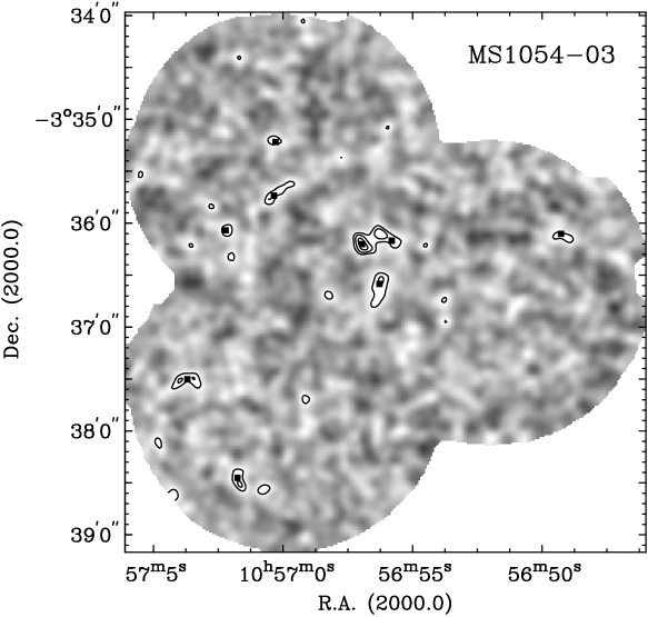
Figure 7: The signal-to-noise 850 $\mu$m SCUBA map of the cluster MS1054-03. The overlayed contours represent $S/N=$ 3,4,5,6,7,8. The black boxes indicate the positions of the detected sources. To cover a large area of the existing multi-wavelength data (see text for details), we have obtained three pointings for this field.

MS1054$-$03   For this cluster the deepest multi-wavelength data set exists, ranging from radio to X-ray. It is a part of the FIRES-project (Faint IR Extragalactic Survey; Franx et al., 2000; Förster Schreiber et al., 2006), which includes the deepest near-IR imaging of a cluster taken with ISAAC at VLT. The area covered with ISAAC and other instruments is about 5${}^{\prime}\times$5^′, so we decided to obtain three pointings to cover a larger area of the field and take advantage of the excellent data available for follow-up studies. The three pointings, which are denoted by $S$, $N$ and $NW$, according to the relative position cover a signification part of the FIRES field. The $S$ pointing is centered at the cluster centre. We detect nine sources with fluxes between 3.5 and 5.0 mJy. We note that one source has more than 5 per cent of their posterior probability distribution below 0 mJy, however, this source has already been identified with a Distant Red Galaxy at redshift $z=2.423$ (van Dokkum et al., 2004; Knudsen et al., 2005) and thus we do not consider this a spurious detection. The largest fraction of the sources are located in the $N$ pointing, while the $NW$ pointing is a lot sparser. This suggests a level of clustering of SCUBA sources, though the field is too small for a reliable clustering analysis. Our map is about three times deeper than the shallow map of the area of the $S$-pointing published by Chapman et al. (2002). They find one source, which is off-set $\sim$ 25^′′ north of SMM J105703.7$-$033730 and not at all detected in our much deeper map. The gravitational lensing is not particularly strong for this cluster, which is partly related to the relative high redshift. The mass model is based on the overall cluster potential (Tran et al. 1999; P. van Dokkum, private communication).

A1689   With $\sim$ 34 hours raw integration time for a single pointing and a 1$\sigma$ r.m.s. $\sim$ 0.7 mJy, this is one of the deepest maps of the survey. A1689 is a cluster known to have an exceptionally large Einstein radius (e.g., King et al., 2002). Because the gravitational lensing is so strong, the source plane area at redshift $z=$ 2.5 is only 0.3 arcmin², i.e. 20 times smaller than the image plane area or the field of view of SCUBA. We detect nine SCUBA sources, and note that this field might be suffering from confusion due to the large number of sources. The three central sources are approximately one beam from one another, and the same is the case for two eastern sources. The sources have observed fluxes between 2.6 and 5.4 mJy. When correcting for the gravitational lensing magnification the fluxes are between 0.11 and 1.3 mJy. The central source SMM J131129.1$-$012049 has a probable detection of 450 $\mu$m flux.
Two multiply-imaged galaxies have been identified among the submm galaxies in this field. SMM J131129.1$-$012049 and SMM J131134.1$-$012021 have been identified with the triple-imaged system 5 (as numbered in Broadhurst et al. (2005)), while SMM J131132.0$-$011955, SMM J131129.8$-$012037 and a small contribution to SMM J131134.1$-$012021 arise from either system 24 or 29, both quintuple-imaged galaxies. Recent optical spectroscopy has shown that all these galaxies have redshifts $\sim 2.5$ (Knudsen et al., in prep., and Richard et al., in prep.). A detailed analysis of the identification will be discussed in a future paper along with additional multi-wavelength follow-up. The mass model will be presented in detail in Richard et al. (in prep.) and Limousin et al. (submitted).

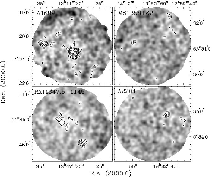
Figure 8: The signal-to-noise ($S/N$) 850 $\mu$m SCUBA maps of the clusters A1689, MS1358+62, RX J1347.5-1145 and A2204. The overlayed contours represent $S/N=$ 3,4,5,6,7,8. The stars $\star$ indicate the positions of the detected sources.

RX J1347.5$-$1145   This is the most X-ray-luminous cluster known (Allen et al., 2002). In this field we detect one source, SMM J134728.0$-$114556, which has $S_{850}=$ 16.2$\pm$3.1 mJy and $S_{450}=$ 98.7$\pm$29.6 mJy. The source is strongly lensed and has an unlensed flux of 4.5 mJy. Furthermore, a large, extended source near the cluster centre is present. This is the Sunyaev–Zel’dovich effect reported in Komatsu et al. (1999). The mass model is based on Cohen & Kneib (2002).

MS1358+62 This map is relatively empty with only one detection SMM J135957.1+623114, with $S_{850}=$ 6.8$\pm$1.3 mJy; 4.4 mJy after correcting for the lensing. These data were first obtained to study the strongly lensed, redshift $z=$ 4.92 galaxy MS1358+62-G1 (Franx et al., 1997), which however was not detected (van der Werf et al., 2001). We here find a 3$\sigma$ upper limit for G1 of $S_{850}<$ 4.8 mJy. A detailed mass model describes the potential for this cluster (Franx et al., 1997; Santos et al., 2004).

A2204   This field has the shallowest SCUBA observations of the whole survey. One point source, SMM J163244.7+053452, has been detected at a $S/N=$ 4.9 with an observed flux of $S_{850}=$ 22.2$\pm$5.7 mJy making it the second brightest source in the catalogue. This source is lensed by more than a factor 3, resulting in a corrected flux of $\sim$ 7 mJy.

A2218   Together with A1689 and the NTT Deep Field, this field is the deepest data taken for the survey. The data for this field cover an area corresponding to more than two pointings. The data was used as a case study for the source extraction method, the Mexican Hat Wavelets algorithm, applied for this survey (Knudsen et al., 2006).

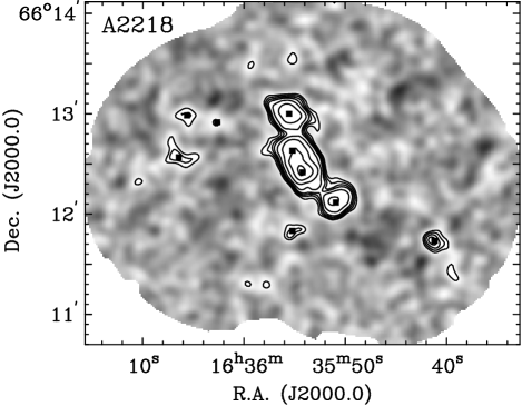
Figure 9: The signal-to-noise 850 $\mu$m SCUBA map of the cluster A2218. The overlayed contours represent $S/N=$ 3,4,5,6,8,12,18,24. The black boxes indicate the positions of the detected sources.

In this field nine sources were detected. The three source, SMM J163550.9+661207, SMM J163554.2+661225 and SMM J163555.2+661238, have been identified as the same, multiply-image source at redshift $z=$ 2.516 (Kneib et al., 2004), and is referred to as SMM J16359+6612. The source SMM J163555.2+661150, which is detected both at 850 $\mu$m and 450 $\mu$m, is coincident with a known galaxy, #289, with redshift $z=$ 1.034 (Pello et al., 1992) and is also detected at 15 $\mu$m with ISOCAM (e.g., Metcalfe et al., 2003). The relatively bright source SMM J163541.2+661144 is detected at both 850 $\mu$m and 450 $\mu$m. The sources in A2218 have observed fluxes between 2.8 and 16.1 mJy. The lensing corrected fluxes are 0.4–6.1 mJy. The mass model is based on Kneib et al. (1996); Ellis et al. (2001); Kneib et al. (2004).

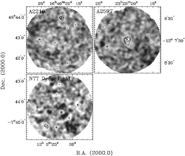
Figure 10: The signal-to-noise ($S/N$) 850 $\mu$m SCUBA maps of the clusters A2219 and A2597 and of the blank field NTT Deep Field. The overlayed contours represent $S/N=$ 3,4,5,6. The stars $\star$ indicate the positions of the detected sources.

A2219   In this field we detect two point sources that both have possible detections of 450 $\mu$m flux. This field was also a part of the Chapman et al. (2002) sample, though their observations are shallower. The source SMM 164019.5+464358 agrees well with their finding. In Chapman et al. (2002) the source C SMM J16404+4643 has an upper limit at 850 $\mu$m, while being detected at 450 $\mu$m. We do not get a significant detection of the source, but MHW does suggest a $S/N\sim$ 1.9 detection, which corresponds to a flux of $\sim$ 2.3 mJy; the 3$\sigma$ upper limit is $<$ 3.6 mJy. We note that one source has more than 5 per cent of its posterior probability distribution below 0 mJy. For the source B SMM J16403+46437 MHW suggests a $S/N\sim$ 2.3 detection. The source D SMM J16404+4644 is within the edge region which have trimmed from the map. In our map a positive fluctuation is present, though it does not have the characteristics of a significant 850 $\mu$m detection. Furthermore, MHW also finds a $S/N\sim$ 2.9 source at $\alpha,\delta$ = 16^h40^m22^s,+46^∘42^′25^′′. The mass model is described in Smith et al. (2005).

A2597   In this field, two point sources were detected with $S/N>$ 3. The brightest source, SMM J232519.8$-$120727, is a 12 mJy source located in the centre of the map and is coincident with the cD galaxy of the cluster, which is a well-known AGN (e.g., McNamara et al., 1999). The cD galaxy is excluded from the rest of the analysis in this paper. The other source, SMM 232523.4$-$120745, is a 5 mJy source, which also has detected 450 $\mu$m flux. We note that this source has more than 5 per cent of their posterior probability distribution below 0 mJy. Hence, if this is indeed a spurious source, then no high-$z$ background sources were detected in this field. The mass model includes both the overall potential of the cluster and that of the cD galaxy (Smith et al., 1990; Wu & Xue, 2000).

NTT Deep Field   This field, the blank field of the survey (Arnouts et al., 1999). is one of the deepest fields of the survey. Five sources have been detected with fluxes between 3 and 4 mJy. None of them have detected 450 $\mu$m flux. In Figure 10, source SMM J120520.6$-$074448 has no $S/N=$ 3 contour as it is located in a depression in the background. A 1.2 millimeter map of the NTT Deep Field has been obtained with the Max-Planck Millimetre Bolometer (MAMBO) covering a larger area of the NTT Deep Field than the SCUBA map presented here (Dannerbauer et al., 2002, 2004). Considering that 1.2 mm probes a part of the modified blackbody where the flux is fainter compared to the 850 $\mu$m, the MAMBO map is a bit shallower than the deep SCUBA map. Two MAMBO sources are covered by the SCUBA map. The source MM J120517$-$0743.1 is very close to the edge of the SCUBA map, where there are no indications of a source. The source MM J120522$-$0745.1, which has a radio detection, is only 6^′′ from the submm source SMM J120523.1$-$074516. The radio detection is coincident with the submm source.

References

- Allen et al. (1993) Allen S. W., Fabian A. C., Johnstone R. M., White D. A., Daines S. J., Edge A. C., Stewart G. C., 1993, MNRAS, 262, 901
- Allen et al. (2002) Allen S. W., Schmidt R. W., Fabian A. C., 2002, MNRAS, 335, 256
- Archibald et al. (2000) Archibald E. N., Wagg J. W., Jenness T., , 2000, SCD System Note 2.2, http://www.jach.hawaii.edu/JACdocs/JCMT/SCD/SN/002.2/
- Arnouts et al. (1999) Arnouts S., D’Odorico S., Cristiani S., Zaggia S., Fontana A., Giallongo E., 1999, A&A, 341, 641
- Barger et al. (1999) Barger A. J., Cowie L. L., Sanders D. B., 1999, ApJ, 518, L5
- Barnard et al. (2004) Barnard V. E., Vielva P., Pierce-Price D. P. I., Blain A. W., Barreiro R. B., Richer J. S., Qualtrough C., 2004, MNRAS, 352, 961
- Blain (2001) Blain A. W., 2001, in Cristiani S., Renzini A., Williams R. E., eds, Deep Fields SCUBA Deep Fields and Source Confusion. p. 129
- Blain et al. (1999) Blain A. W., Smail I., Ivison R. J., Kneib J.-P., 1999, MNRAS, 302, 632
- Blain et al. (1999) Blain A. W., Kneib J.-P., Ivison R. J., Smail I., 1999, ApJ, 512, L87
- Borys et al. (2004) Borys C., Chapman S., Donahue M., Fahlman G., Halpern M., Kneib J.-P., Newbury P., Scott D., Smith G. P., 2004, MNRAS, 352, 759
- Borys et al. (2003) Borys C., Chapman S., Halpern M., Scott D., 2003, MNRAS, 344, 385
- Borys et al. (2004) Borys C., Scott D., Chapman S., Halpern M., Nandra K., Pope A., 2004, MNRAS, 355, 485
- Broadhurst et al. (2005) Broadhurst T., et al., 2005, ApJ, 621, 53
- Carlberg et al. (1996) Carlberg R. G., Yee H. K. C., Ellingson E., Abraham R., Gravel P., Morris S., Pritchet C. J., 1996, ApJ, 462, 32
- Cayón et al. (2000) Cayón L., Sanz J. L., Barreiro R. B., Martínez-González E., Vielva P., Toffolatti L., Silk J., Diego J. M., Argüeso F., 2000, MNRAS, 315, 757
- Chapman et al. (2003) Chapman S. C., Blain A. W., Ivison R. J., Smail I. R., 2003, Nature, 422, 695
- Chapman et al. (2005) Chapman S. C., Blain A. W., Smail I., Ivison R. J., 2005, ApJ, 622, 772
- Chapman et al. (2002) Chapman S. C., Scott D., Borys C., Fahlman G. G., 2002, MNRAS, 330, 92
- Chapman et al. (2000) Chapman S. C., Scott D., Steidel C. C., Borys C., Halpern M., Morris S. L., Adelberger K. L., Dickinson M., Giavalisco M., Pettini M., 2000, MNRAS, 319, 318
- Cohen & Kneib (2002) Cohen J. G., Kneib J.-P., 2002, ApJ, 573, 524
- Condon (1974) Condon J. J., 1974, ApJ, 188, 279
- Coppin et al. (2006) Coppin K., et al., 2006, MNRAS, 372, 1621
- Coppin et al. (2005) Coppin K., Halpern M., Scott D., Borys C., Chapman S., 2005, MNRAS, 357, 1022
- Cowie et al. (2002) Cowie L. L., Barger A. J., Kneib J.-P., 2002, AJ, 123, 2197
- Dannerbauer et al. (2002) Dannerbauer H., Lehnert M. D., Lutz D., Tacconi L., Bertoldi F., Carilli C., Genzel R., Menten K., 2002, ApJ, 573, 473
- Dannerbauer et al. (2004) Dannerbauer H., Lehnert M. D., Lutz D., Tacconi L., Bertoldi F., Carilli C., Genzel R., Menten K. M., 2004, ApJ, 606, 664
- Eales et al. (2000) Eales S., Lilly S., Webb T., Dunne L., Gear W., Clements D., Yun M., 2000, AJ, 120, 2244
- Edge et al. (1999) Edge A. C., Ivison R. J., Smail I., Blain A. W., Kneib J.-P., 1999, MNRAS, 306, 599
- Ellis et al. (2001) Ellis R., Santos M. R., Kneib J.-P., Kuijken K., 2001, ApJ, 560, L119
- Fixsen et al. (1998) Fixsen D. J., Dwek E., Mather J. C., Bennett C. L., Shafer R. A., 1998, ApJ, 508, 123
- Förster Schreiber et al. (2006) Förster Schreiber N. M., et al., 2006, AJ, 131, 1891
- Franx et al. (1997) Franx M., Illingworth G. D., Kelson D. D., van Dokkum P. G., Tran K.-V., 1997, ApJ, 486, L75
- Franx et al. (2000) Franx M., et al., 2000, The Messenger, 99, 20
- Garrett et al. (2005) Garrett M. A., Knudsen K. K., van der Werf P. P., 2005, A&A, 431, L21
- Gehrels (1986) Gehrels N., 1986, ApJ, 303, 336
- Govoni et al. (2001) Govoni F., Feretti L., Giovannini G., Böhringer H., Reiprich T. H., Murgia M., 2001, A&A, 376, 803
- Högbom (1974) Högbom J. A., 1974, A&AS, 15, 417
- Hogg (2001) Hogg D. W., 2001, AJ, 121, 1207
- Holland et al. (1999) Holland W. S., et al., 1999, MNRAS, 303, 659
- Hughes et al. (1998) Hughes D. H., et al., 1998, Nature, 394, 241
- Jenness & Lightfoot (1998) Jenness T., Lightfoot J. F., 1998, in Albrecht R., Hook R. N., Bushouse H. A., eds, ASP Conf. Ser. 145: Astronomical Data Analysis Software and Systems VII Reducing SCUBA Data at the James Clerk Maxwell Telescope. p. 216
- King et al. (2002) King L. J., Clowe D. I., Schneider P., 2002, A&A, 383, 118
- Kneib et al. (1996) Kneib J.-P., Ellis R. S., Smail I., Couch W. J., Sharples R. M., 1996, ApJ, 471, 643
- Kneib et al. (1993) Kneib J. P., Mellier Y., Fort B., Mathez G., 1993, A&A, 273, 367
- Kneib et al. (2005) Kneib J.-P., Neri R., Smail I., Blain A., Sheth K., van der Werf P., Knudsen K. K., 2005, A&A, 434, 819
- Kneib et al. (2004) Kneib J.-P., van der Werf P. P., Kraiberg Knudsen K., Smail I., Blain A., Frayer D., Barnard V., Ivison R., 2004, MNRAS, 349, 1211
- Knudsen et al. (2006) Knudsen K. K., et al., 2006, MNRAS, 368, 487
- Knudsen et al. (2005) Knudsen K. K., et al., 2005, ApJ, 632, L9
- Knudsen et al. (2003) Knudsen K. K., van der Werf P. P., Jaffe W., 2003, A&A, 411, 343
- Komatsu et al. (1999) Komatsu E., Kitayama T., Suto Y., Hattori M., Kawabe R., Matsuo H., Schindler S., Yoshikawa K., 1999, ApJ, 516, L1
- (51) Maloney P. R., et al., 2005, ApJ, 635, 1044
- McNamara et al. (1999) McNamara B. R., Jannuzi B. T., Sarazin C. L., Elston R., Wise M., 1999, ApJ, 518, 167
- Metcalfe et al. (2003) Metcalfe L., et al., 2003, A&A, 407, 791
- Peletier et al. (1990) Peletier R. F., Davies R. L., Illingworth G. D., Davis L. E., Cawson M., 1990, AJ, 100, 1091
- Pello et al. (1992) Pello R., Le Borgne J. F., Sanahuja B., Mathez G., Fort B., 1992, A&A, 266, 6
- Proust et al. (2000) Proust D., Cuevas H., Capelato H. V., Sodré Jr. L., Tomé Lehodey B., Le Fèvre O., Mazure A., 2000, A&A, 355, 443
- Puget et al. (1996) Puget J.-L., Abergel A., Bernard J.-P., Boulanger F., Burton W. B., Desert F.-X., Hartmann D., 1996, A&A, 308, L5
- Santos et al. (2004) Santos M. R., Ellis R. S., Kneib J.-P., Richard J., Kuijken K., 2004, ApJ, 606, 683
- Sawicki & Webb (2005) Sawicki M., Webb T. M. A., 2005, ApJ, 618, L67
- Scott et al. (2006) Scott S. E., Dunlop J. S., Serjeant S., 2006, MNRAS, 370, 1057
- Scott et al. (2002) Scott S. E., et al., 2002, MNRAS, 331, 817
- Serjeant et al. (2003) Serjeant S., et al., 2003, MNRAS, 344, 887
- Sheth et al. (2004) Sheth K., Blain A. W., Kneib J.-P., Frayer D. T., van der Werf P. P., Knudsen K. K., 2004, ApJ, 614, L5
- Smail et al. (1997) Smail I., Ivison R. J., Blain A. W., 1997, ApJ, 490, L5
- Smail et al. (2002) Smail I., Ivison R. J., Blain A. W., Kneib J.-P., 2002, MNRAS, 331, 495
- Smith et al. (1990) Smith E. P., Heckman T. M., Illingworth G. D., 1990, ApJ, 356, 399
- Smith et al. (2005) Smith G. P., Kneib J.-P., Smail I., Mazzotta P., Ebeling H., Czoske O., 2005, MNRAS, 359, 417
- Tran et al. (1999) Tran K.-V. H., Kelson D. D., van Dokkum P., Franx M., Illingworth G. D., Magee D., 1999, ApJ, 522, 39
- van der Werf et al. (2001) van der Werf P. P., Knudsen K. K., Labbé I., Franx M., 2001, in Lowenthal J. D., Hughes D. H., eds, Deep Millimeter Surveys: Implications for Galaxy Formation and Evolution Can Dusty Lyman Break Galaxies Produce the Submillimeter Counts and Background? Lessons from Lensed Lyman Break Galaxies. p. 103
- van Dokkum et al. (2004) van Dokkum P. G., et al., 2004, ApJ, 611, 703
- (71) Wang W.-H., Cowie, L. L., Barger, A. J., 2006, ApJ, 647, 74
- Webb et al. (2003) Webb T. M., et al., 2003, ApJ, 582, 6
- Webb et al. (2003) Webb T. M., Eales S. A., Lilly S. J., Clements D. L., Dunne L., Gear W. K., Ivison R. J., Flores H., Yun M., 2003, ApJ, 587, 41
- Webb et al. (2004) Webb T. M. A., Brodwin M., Eales S., Lilly S. J., 2004, ApJ, 605, 645
- Webb et al. (2005) Webb T. M. A., Yee H. K. C., Ivison R. J., Hoekstra H., Gladders M. D., Barrientos L. F., Hsieh B. C., 2005, ApJ, 631, 187
- Wehner et al. (2002) Wehner E. H., Barger A. J., Kneib J.-P., 2002, ApJ, 577, L83
- White et al. (1991) White D. A., Fabian A. C., Johnstone R. M., Mushotzky R. F., Arnaud K. A., 1991, MNRAS, 252, 72
- White et al. (1997) White D. A., Jones C., Forman W., 1997, MNRAS, 292, 419
- Wu & Xue (2000) Wu X.-P., Xue Y.-J., 2000, ApJ, 542, 578
- Zabludoff et al. (1990) Zabludoff A. I., Huchra J. P., Geller M. J., 1990, ApJS, 74, 1