Poisson Matching

Abstract

Suppose that red and blue points occur as independent homogeneous Poisson processes in ${\mathbb{R}}^{d}$. We investigate translation-invariant schemes for perfectly matching the red points to the blue points. For any such scheme in dimensions $d=1,2$, the matching distance $X$ from a typical point to its partner must have infinite $d/2$-th moment, while in dimensions $d\geq 3$ there exist schemes where $X$ has finite exponential moments. The Gale-Shapley stable marriage is one natural matching scheme, obtained by iteratively matching mutually closest pairs. A principal result of this paper is a power law upper bound on the matching distance $X$ for this scheme. A power law lower bound holds also. In particular, stable marriage is close to optimal (in tail behavior) in $d=1$, but far from optimal in $d\geq 3$. For the problem of matching Poisson points of a single color to each other, in $d=1$ there exist schemes where $X$ has finite exponential moments, but if we insist that the matching is a deterministic factor of the point process then $X$ must have infinite mean.

1 Introduction

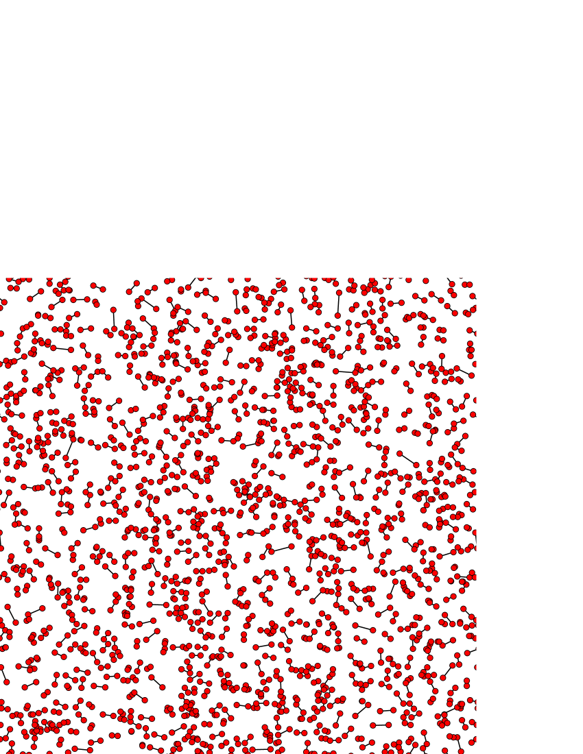
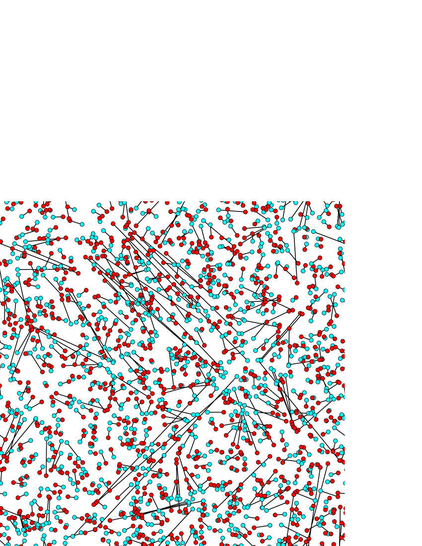
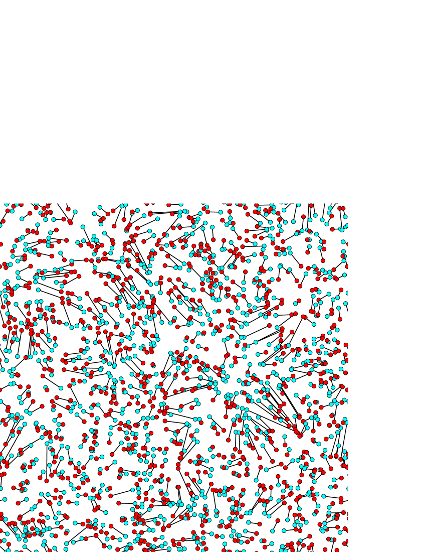
Figure 1: Matchings of 2000 uniformly random points on a 2-dimensional torus: (i) stable 1-color; (ii) minimum-length 1-color; (iii) stable 2-color; (iv) minimum-length 2-color.

Let ${\cal R}$ be a simple point process of finite intensity in ${\mathbb{R}}^{d}$. The support of ${\cal R}$ is the random set $[{\cal R}]:=\{x\in{\mathbb{R}}^{d}:{\cal R}(\{x\})=1\}$. Elements of $[{\cal R}]$ are called red points. A one-color matching scheme of ${\cal R}$ is a simple point process ${\cal M}$ of unordered pairs $\{x,y\}\subset{\mathbb{R}}^{d}$, on a shared probability space, such that almost surely $(V,E)=([{\cal R}],[{\cal M}])$ is a random graph which is a perfect matching of $[{\cal R}]$ (i.e. a simple graph with all degrees 1). Let ${\cal B}$ be a second simple point process, and call elements of $[{\cal B}]$ blue points. A two-color matching scheme between ${\cal R}$ and ${\cal B}$ is a process ${\cal M}$ which similarly yields almost surely a perfect bipartite matching between $[{\cal R}]$ and $[{\cal B}]$ (i.e. a perfect matching of $[{\cal R}]\cup[{\cal B}]$ where all the edges are from $[{\cal R}]$ to $[{\cal B}]$). In either case we denote by ${\cal M}(x)$ the partner of a red or blue point $x$; that is the unique point such that $\{x,{\cal M}(x)\}\in[{\cal M}]$. See Figure 1 for some examples on the finite torus.

We say that a one-color (respectively two-color) matching scheme ${\cal M}$ is translation-invariant if the law of the joint process $({\cal R},{\cal M})$ (respectively $({\cal R},{\cal B},{\cal M})$) is invariant under translations of ${\mathbb{R}}^{d}$. Isometry-invariance is defined analogously. If almost surely ${\cal M}=f({\cal R})$ (respectively ${\cal M}=f({\cal R},{\cal B})$) for some deterministic function $f$ then we call ${\cal M}$ a factor matching scheme. We sometimes refer to a matching scheme which is not a factor as randomized.

For a translation-invariant one-color or two-color matching scheme, let ${\mathbb{P}}$ be the probability measure governing $({\cal R},{\cal M})$ or $({\cal R},{\cal B},{\cal M})$, and ${\mathbb{E}}$ the associated expectation operator. We are interested in the typical distance between matched pairs. Assume without loss of generality that ${\cal R}$ has intensity $1$ (otherwise rescale). For $r\in[0,\infty]$ it is natural to consider the quantity

$$F(r):={\mathbb{E}}\#\big{\{}x\in[{\cal R}]\cap[0,1)^{d}:|x-{\cal M}(x)|\leq r\big{\}},$$

where $|\cdot|$ denotes the Euclidean norm. It is easy to see that $F$ is a distribution function, therefore we introduce a random variable $X$ with probability measure ${\mathbb{P}}^{*}$ and expectation operator ${\mathbb{E}}^{*}$ such that

$${\mathbb{P}}^{*}(X\leq r)=F(r).$$ (1)

We can think of $X$ as the typical distance from a red point to its partner. In fact, this interpretation can be made rigorous via the technology of Palm processes – see Section 2 below.

We consider the following main questions. For Poisson processes on ${\mathbb{R}}^{d}$, what is the best possible tail behavior (as measured by $X$) for a translation-invariant (or isometry-invariant) matching scheme, in the one-color and two-color cases? How do the answers depend on dimension? And if we insist on a factor matching scheme? We also address the case of stable matchings – see below.

Note the following trivial lower bound on $X$. In the one-color or two-color case, the partner of a point must be at least as far as the closest other point. In the case when ${\cal R}$ (respectively ${\cal R}+{\cal B}$) is a homogeneous Poisson process, this gives

$${\mathbb{E}}^{*}e^{cX^{d}}=\infty$$ (2)

for some $c=c(d)\in(0,\infty)$.

The following theorems show that the optimal tail behavior of two-color matching schemes depends dramatically on the dimension.

Theorem 1 (2-color upper bounds).

Let ${\cal R},{\cal B}$ be independent Poisson processes of intensity 1. There exist isometry-invariant two-color matching schemes satisfying:

• in $d=1$: ${\mathbb{P}}^{*}(X>r)\leq Cr^{-1/2}\quad\forall r>0;$

• in $d=2$: ${\mathbb{P}}^{*}(X>r)\leq Cr^{-1}\quad\forall r>0;$

• in $d\geq 3$: ${\mathbb{E}}^{*}e^{CX^{d}}<\infty.$

Here $C=C(d)\in(0,\infty)$ denotes a constant. Furthermore, in (i) the matching scheme is a factor.

Theorem 2 (2-color lower bounds; [14]).

Let ${\cal R},{\cal B}$ be independent Poisson processes of intensity 1. In $d=1$ or $d=2$, any translation-invariant two-color matching scheme (factor or not) satisfies

$${\mathbb{E}}^{*}X^{d/2}=\infty.$$

Together with the trivial bound (2), Theorems 1 and 2 settle reasonably accurately the question of optimal tail behavior for randomized two-color matchings. We do not know the optimal tail behavior for translation-invariant factor matching schemes of two independent Poisson processes in dimensions $d\geq 2$. Theorem 2 was derived in [14] via results from [17, 12], the proofs of which were quite involved. We will present here a simple direct proof.

Here is a brief heuristic explanation for the above tail behavior, and in particular the sharp difference between dimensions $d\leq 2$ and $d\geq 3$. In a ball of large radius $r$, the discrepancy between the numbers of red and blue points is typically a random multiple of $r^{d/2}$ (by the central limit theorem). This discrepancy must be accommodated via the boundary of the ball, which has size of order $r^{d-1}$. When $d\leq 2$, the discrepancy exceeds the boundary (with substantial probability), so we expect that a fraction $r^{d/2}/r^{d}=r^{-d/2}$ of points must be matched at distance at least of order $r$. When $d\geq 3$, the boundary exceeds the discrepancy, so far more efficient matching is possible, with the tails determined by local deviations in the distribution of points.

The following illustrates a case where allowing additional randomization makes a striking difference to tail behavior.

Theorem 3 (1-color, 1 dimension).

Let $d=1$, let ${\cal R}$ be a Poisson process of intensity 1, and consider one-color matching schemes.

• Any translation-invariant factor matching satisfies ${\mathbb{E}}^{*}X=\infty.$

• There exists an isometry-invariant randomized scheme satisfying ${\mathbb{P}}^{*}(X>r)=e^{-r}\quad\forall r>0.$

The following shows that the above dichotomy does not extend to higher dimensions.

Theorem 4 (1-color, 2 or more dimensions).

Let ${\cal R}$ be a Poisson process of intensity 1. For all $d\geq 2$ there exists a translation-invariant one-color factor matching scheme satisfying

$${\mathbb{E}}^{*}e^{CX^{d}}<\infty,$$

for some $C=C(d)\in(0,\infty)$. The same bound can be attained by a randomized isometry-invariant matching scheme in all $d\geq 2$, and by an isometry-invariant factor matching scheme in $d=2$.

We do not know how to construct an isometry-invariant factor matching satisfying the bound in Theorem 4 for $d\geq 3$ (see the remarks in Section 4, however).

Stable matching: Iterated mutually closest matching algorithm.

The following natural “greedy” algorithm gives a matching scheme by trying to optimize locally. When considering a two-color matching, call a pair of points $x,y$ potential partners if one is red while the other is blue. In the one-color case, call $x$ and $y$ potential partners if they are distinct points in $[{\cal R}]$. We say that potential partners $x$ and $y$ are mutually closest if $y$ is the closest potential partner to $x$ and $x$ is the closest potential partner to $y$. Now, given the point configuration, match all mutually closest pairs to each other, then remove these points and match all mutually closest pairs in the remaining set of points. Repeat indefinitely. $\Diamond$

It turns out that the above algorithm yields a perfect matching under general conditions (Proposition 9), and in particular this holds almost surely in the case when ${\cal R}$ is a Poisson process (and for the two-color case, when ${\cal B}$ is an independent Poisson process of the same intensity). Furthermore, it is the unique stable matching in the sense of Gale and Shapley [8]. (See Section 2 for the details). Evidently (under the aforementioned conditions) the stable matching gives an isometry-invariant factor matching scheme.

We can accurately describe the tail behavior of stable matchings in the one-color case, but some questions remain in the two-color case.

Theorem 5 (1-color stable matching).

Let ${\cal R}$ be a Poisson process of intensity $1$. For any $d\geq 1$, the one-color stable matching satisfies

• ${\mathbb{E}}^{*}X^{d}=\infty;$

• ${\mathbb{P}}^{*}(X>r)\leq Cr^{-d}\quad{\forall r>0};$

for some $C=C(d)\in(0,\infty)$.

Theorem 6 (2-color stable matching).

Let ${\cal R},{\cal B}$ be independent Poisson processes of intensity $1$. For $d\geq 1$, the two-color stable matching satisfies:

• ${\mathbb{E}}^{*}X^{d}=\infty$,
  (Theorem 2 gives a better bound in $d=1,2$);

• ${\mathbb{P}}^{*}(X>r)\leq Cr^{-s}\quad{\forall r>0},$
  where $s=s(d)\in(0,1)$ satisfies $s(1)=1/2$, and $C=C(d)\in(0,\infty)$.

The power $s(d)$ is given explicitly as the solution of an equation, and for example $s(2)=0.496\cdots$ and $s(3)=0.449\cdots$ – see Theorem 19. It is a fascinating unsolved question to determine the correct power law for $d\geq 2$ (see the open problems at the end of the article).

It is interesting that stable matching performs essentially optimally (in terms of tail behavior) among (possibly randomized) matching schemes in the two-color case for $d=1$, but not for $d\geq 3$, and not in the one-color case.

Summary

The following tables summarize the best known results for isometry-invariant matchings of Poisson processes.

1-color matching		Lower bound		Upper bound /
				best construction
Randomized	All $d$	${\mathbb{E}}^{*}e^{cX^{d}}=\infty$	$\approx$	${\mathbb{E}}^{*}e^{CX^{d}}<\infty$
Factor	$d=1$	${\mathbb{E}}^{*}X=\infty$	$\approx$	[${\mathbb{P}}^{*}(X>r)\leq Cr^{-1}$]
	$d\geq 2$	${\mathbb{E}}^{*}e^{cX^{d}}=\infty$	$\approx$	${\mathbb{E}}^{*}e^{CX^{d}}<\infty$ ((T) for $d\geq 3$)
Stable	All $d$	${\mathbb{E}}^{*}X^{d}=\infty$	$\approx$	${\mathbb{P}}^{*}(X>r)\leq Cr^{-d}$

2-color matching		Lower bound		Upper bound /
				best construction
Randomized	$d=1,2$	${\mathbb{E}}^{*}X^{d/2}=\infty$	$\approx$	${\mathbb{P}}^{*}(X>r)\leq Cr^{-d/2}$
	$d\geq 3$	${\mathbb{E}}^{*}e^{cX^{d}}=\infty$	$\approx$	${\mathbb{E}}^{*}e^{CX^{d}}<\infty$
Factor	$d=1$	[${\mathbb{E}}^{*}X^{1/2}=\infty$]	$\approx$	[${\mathbb{P}}^{*}(X>r)\leq Cr^{-1/2}$]
	$d=2$	[${\mathbb{E}}^{*}X=\infty$]	$\ll$	$[{\mathbb{P}}^{*}(X>r)\leq Cr^{-0.496\cdots}]$
	$d\geq 3$	${\mathbb{E}}^{*}e^{cX^{d}}=\infty$	$\ll$	$[{\mathbb{P}}^{*}(X>r)\leq Cr^{-s(d)}]$
Stable	$d=1$	[${\mathbb{E}}^{*}X^{1/2}=\infty$]	$\approx$	${\mathbb{P}}^{*}(X>r)\leq Cr^{-1/2}$
	$d=2$	[${\mathbb{E}}^{*}X=\infty$]	$\ll$	${\mathbb{P}}^{*}(X>r)\leq Cr^{-0.496\cdots}$
	$d\geq 3$	${\mathbb{E}}^{*}X^{d}=\infty$	$\ll$	${\mathbb{P}}^{*}(X>r)\leq Cr^{-s(d)}$

Notes:
(T)	Translation-invariant scheme only.
[$\cdots$]	Bound follows from line above (lower bounds)
	or below (upper bounds).
$\approx$	Indicates reasonably close lower and upper bounds.
$\ll$	Indicates a substantial gap between the lower
	and upper bounds.

Extensions to other processes

The results on 2-color matchings in Theorems 1, 2, 6 all extend, with similar proofs, to the following two variant settings.

• Perfect matchings of Heads to Tails for i.i.d. fair coin flips indexed by ${\mathbb{Z}}^{d}$ (see [14, 18, 20] for details). (In order to define stable matchings in this context, one must specify a way to break ties between pairs of sites ${\mathbb{Z}}^{d}$ which are the same distance apart). Here the random variable $X$ denotes the distance from the origin to its partner.

• Fair allocations of Lebesgue measure to a Poisson process (see [11] and also [5, 10, 14] for definitions and background). Here $X$ denotes the distance from the origin to its allocated Poisson point. The resulting upper bounds on the stable allocation in Theorem 6(ii) represent a considerable improvement on the previous best results: $X$ was known to have finite $(1/18)$th moment in $d=1$, and no quantitative upper bound was known in $d\geq 2$ [10].

Where appropriate, we make remarks following the proofs regarding the adaptation of our results to these settings.

Some of our results extend easily to point processes other than the Poisson process. In particular, Theorem 5(ii) holds for any translation-invariant simple point process for which the stable matching is well-defined (see Proposition 9). Theorems 5(i) and 6(i) hold provided in addition the point processes are tolerant of local modifications (see Proposition 18).

Another interesting variant concerns matching of random points on large finite boxes; see e.g. [1, 3, 7, 19]. We do not explore this connection in depth, but our proof of Theorem 1(iii) relies on the remarkable results of [19].

2 Preliminaries

In this section we present some useful elementary definitions and results.

Some notation

Let ${\mathcal{L}}$ denote Lebesgue measure on ${\mathbb{R}}^{d}$, and denote the Euclidean ball $B(x,r)$ $:=\{z\in{\mathbb{R}}^{d}:|x-z|<r\}$. We denote the unit cube $Q:=[0,1)^{d}\subset{\mathbb{R}}^{d}$, and $Q_{u}:=Q+u$ for $u\in{\mathbb{Z}}^{d}$.

Palm processes

Consider a translation-invariant one-color or two-color matching scheme, and let ${\mathbb{P}}$ be the probability measure governing $({\cal R},{\cal M})$ or $({\cal R},{\cal B},{\cal M})$. We introduce the Palm process $({\cal R}^{*},{\cal M}^{*})$ or $({\cal R}^{*},{\cal B}^{*},{\cal M}^{*})$, with law ${\mathbb{P}}^{*}$ and expectation ${\mathbb{E}}^{*}$, in which we condition on the presence of a red point at the origin, while taking ${\cal M}$ and (in the two color-case) ${\cal B}$ as a stationary background. See e.g. [15, Ch. 11] for details. In the case when ${\cal R}$ is a homogeneous Poisson process, it turns out that ${\cal R}^{*}$ has the same distribution as ${\cal R}$ with an added point at the origin:

$$[{\cal R}^{*}]\stackrel{{\scriptstyle d}}{{=}}[{\cal R}]\cup\{0\}.$$ (3)

Also, if ${\cal R}$ and ${\cal B}$ are independent processes then ${\cal R}^{*}$ and ${\cal B}^{*}$ are independent, and ${\cal B}^{*}\stackrel{{\scriptstyle d}}{{=}}{\cal B}$.

If ${\cal R}$ is a translation-invariant measure-valued process of intensity $\lambda\in(0,\infty)$, and $({\cal R}^{*},\Psi^{*})$ is the Palm version of ${\cal R}$ taken together with any jointly translation-invariant random background $\Psi$ (which may be a random function or a random measure on ${\mathbb{R}}^{d}$), then the following properties are standard (see [15, Ch. 11]). Let $\theta^{x}$ denote translation by $x\in{\mathbb{R}}^{d}$ (defined to act on measures via $(\theta^{x}\pi)(S)=\pi(S-x)$ for $S\subseteq{\mathbb{R}}^{d}$). For any measurable $S\subseteq{\mathbb{R}}^{d}$ and any event $A$ we have

$${\mathbb{E}}\int_{S}{\mathbf{1}}\big{[}\theta^{-x}({\cal R},\Psi)\in A\big{]}\;d{\cal R}(x)=\lambda\cdot{\mathcal{L}}S\cdot{\mathbb{P}}^{*}\big{[}({\cal R}^{*},\Psi^{*})\in A\big{]}.$$ (4)

(Indeed this may be taken as a definition of the Palm process). More generally, for any non-negative measurable $f$ on the appropriate space,

$${\mathbb{E}}\int_{{\mathbb{R}}^{d}}f\big{(}\theta^{-x}({\cal R},\Psi),x\big{)}\;d{\cal R}(x)=\lambda\int_{{\mathbb{R}}^{d}}{\mathbb{E}}^{*}f\big{(}({\cal R}^{*},\Psi^{*}),x\big{)}\;dx.$$ (5)

Let ${\cal M}$ be a translation-invariant (one- or two- color) matching scheme. If we let

$$X:=|{\cal M}^{*}(0)|$$ (6)

denote the distance from the origin to its partner under the Palm measure, then (4) yields in particular

$${\mathbb{E}}\#\big{\{}x\in[{\cal R}]\cap S:|x-{\cal M}(x)|\leq r\big{\}}=\lambda\cdot{\mathcal{L}}S\cdot{\mathbb{P}}^{*}(X\leq r).$$ (7)

Hence the above definition of $X$ is consistent with the earlier notation in (1).

Note that the tail bound (2) for the Poisson process is now an elementary consequence of (3) and (6).

Partial matching and mass transport

A partial matching of a set $U$ is the edge set $m$ of a simple graph $(U,m)$ in which each vertex has degree at most 1. As before we write $m(x)=y$ if $\{x,y\}\in m$, and in addition we write $m(x)=\infty$ if $x$ is unmatched (i.e. has degree 0). A one-color (respectively two-color) partial matching scheme ${\cal M}$ is a point process on pairs which yields almost surely a partial matching of $[{\cal R}]$ (respectively between $[{\cal R}]$ and $[{\cal B}]$).

Proposition 7 (Fairness).

Let ${\cal R},{\cal B}$ be simple point processes of finite intensity, and let ${\cal M}$ be a translation-invariant two-color partial matching scheme of ${\cal R}$ and ${\cal B}$. Then the process of matched red points and the process of matched blue points have equal intensity.

In particular, Proposition 7 shows that translation-invariant perfect matching schemes are possible only between two point processes of equal intensity. In addition, by applying the result to the matching obtained by deleting all edges longer than $r$, we see that $X$ is equal in law to the analogous random variable defined in terms of a typical blue point.

We prove Proposition 7 via the following lemma which will be useful elsewhere. (See [4] for background).

Lemma 8 (Mass transport principle).

• Suppose $t:{\mathbb{Z}}^{d}\times{\mathbb{Z}}^{d}\to[0,\infty]$ satisfies $t(u+w,v+w)=t(u,v)$ for all $u,v,w\in{\mathbb{Z}}^{d}$, and write $t(A,B):=\sum_{u\in A,v\in B}t(u,v)$. Then

  $$t(0,{\mathbb{Z}}^{d})=t({\mathbb{Z}}^{d},0).$$

• Suppose $T$ is a random non-negative measure on ${\mathbb{R}}^{d}\times{\mathbb{R}}^{d}$ such that $T(A,B):=T(A\times B)$ and $T(A+w,B+w)$ are equal in law for all $w\in{\mathbb{Z}}^{d}$. Then

  $${\mathbb{E}}T(Q,{\mathbb{R}}^{d})={\mathbb{E}}T({\mathbb{R}}^{d},Q).$$

Proof.

(i): $t(0,{\mathbb{Z}}^{d})=\sum_{u\in{\mathbb{Z}}^{d}}t(0,u)=\sum_{u\in{\mathbb{Z}}^{d}}t(-u,0)=t({\mathbb{Z}}^{d},0).$

(ii): Apply (i) to $t(u,v):={\mathbb{E}}T(Q_{u},Q_{v})$. ∎

We sometimes call $t$ or $T$ a mass transport, and think of $t(A,B)$ or $T(A,B)$ as the amount of mass sent from $A$ to $B$.

Proof of Proposition 7.

Apply Lemma 8 to the mass transport

$$T(A,B):=\#\{x\in[{\cal R}]\cap A:{\cal M}(x)\in B\}$$

in which each matched red point sends unit mass to its partner. Then ${\mathbb{E}}T(Q,{\mathbb{R}}^{d})={\mathbb{E}}\#\{x\in[{\cal R}]\cap Q:{\cal M}(x)\neq\infty\}$, which is the intensity of matched red points, while similarly ${\mathbb{E}}T({\mathbb{R}}^{d},Q)$ is the intensity of matched blue points. ∎

Stable matching

Following Gale and Shapley [8], we say that a partial matching $m$ of a set $U\subset{\mathbb{R}}^{d}$ is stable if there do not exist distinct points $x,y\in U$ satisfying

$$|x-y|<\min\big{\{}|x-m(x)|,|y-m(y)|\big{\}},$$ (8)

where $|x-m(x)|:=\infty$ if $x$ is unmatched. A pair $x,y$ satisfying (8) is called unstable. (The motivation for this definition is that each point prefers to be matched with closer points, so an unstable pair $x,y$ prefer to divorce their current partners and marry each other.) Similarly, a partial bipartite matching between two sets $U,V$ is called stable if there do not exist $x\in U$ and $y\in V$ satisfying (8).

We call a set $U\subset{\mathbb{R}}^{d}$ non-equidistant if there do not exist $w,x,y,z\in U$ with $\{w,x\}\neq\{y,z\}$ and $|w-x|=|y-z|>0$. A descending chain is an infinite sequence $x_{0},x_{1},\ldots\in U$ for which the distances $|x_{i}-x_{i+1}|$ form a strictly decreasing sequence.

Proposition 9 (Unique stable matching).

Let ${\cal R}$ be a translation-invariant homogeneous point processes of finite intensity. (Respectively, let ${\cal R},{\cal B}$ be point processes of equal finite intensity, jointly ergodic under translations). Suppose that almost surely $[{\cal R}]$ (respectively $[{\cal R}]\cup[{\cal B}]$) is non-equidistant, and has no descending chains. Then almost surely there is a unique stable partial matching of $[{\cal R}]$ (respectively between $[{\cal R}]$ and $[{\cal B}]$). Furthermore, it is almost surely a perfect matching, and it is produced by the iterated mutually closest matching algorithm described in the introduction.

Under the conditions in Proposition 9, the stable matching has the following additional interpretation. Grow a ball centered at each red point (respectively, each red point and each blue point) simultaneously, so that at time $t$ all the balls have radius $t$. Whenever two balls touch (respectively, whenever an ${\cal R}$-ball and a ${\cal B}$-ball touch), match their centers to each other, and remove the two balls.

The conditions on the point processes in Proposition 9 hold in particular for homogeneous Poisson processes, as proved in [9]. Clearly, under the conditions of the proposition, the unique stable matching gives an isometry-invariant factor matching scheme. We postpone the proof of Proposition 9 to Section 5.

3 Two-color matching

In this section we give proofs of Theorems 1 and 2.

Proof of Theorem 1(i).

Use the stable matching (see Proposition 9 and Theorem 6(ii)). ∎

Proof of Theorem 1(ii).

We shall give a construction which works in all dimensions, and gives a matching scheme with tails ${\mathbb{P}}^{*}(X>r)\leq Cr^{-d/2}$.

First note that it is sufficient to give a translation-invariant matching satisfying the required bound, for then we may obtain a (randomized) isometry-invariant version by applying a uniformly random isometry preserving the origin (i.e., chosen according to the Haar measure on the compact group of such isometries) to $({\cal R},{\cal B},{\cal M})$. Indeed, it suffices to give a matching scheme which is invariant under translations by elements of ${\mathbb{Z}}^{d}$ and which satisfies

$${\mathbb{E}}\#\{x\in[{\cal R}]\cap Q:|x-{\cal M}(x)|>r\}\leq Cr^{-d/2},$$ (9)

for then we may achieve a translation-invariant version satisfying the same bound by similarly applying a uniformly random translation in the unit cube $Q$.

We start by defining a sequence of successively coarser random partitions of ${\mathbb{R}}^{d}$ into boxes in a ${\mathbb{Z}}^{d}$-invariant way. Let $\tau_{0},\tau_{1},\ldots$ be i.i.d. uniformly random elements of the discrete cube $\{0,1\}^{d}$, independent of the point processes ${\cal R},{\cal B}$. For each $k=0,1,\ldots$, define a $k$-box to be any subset of ${\mathbb{R}}^{d}$ of the form

$$[0,2^{k})^{d}+2^{k}z+\sum_{i=0}^{k-1}2^{i}\tau_{i},$$

where $z\in{\mathbb{Z}}^{d}$.

Now, given the point processes ${\cal R},{\cal B}$ and the partitioning into boxes, define a matching as follows. Within each $0$-box, match as many red/blue pairs as possible in some arbitrary pre-determined way. (For definiteness, choose from among the bipartite partial matchings of maximum cardinality the one which minimizes the total edge length.) Remove those points which have been matched. Now match as many red/blue pairs of the remaining points as possible within each $1$-box, remove these matched points, and repeat for $2$-boxes and so on. The union of all these partial matchings clearly gives a ${\mathbb{Z}}^{d}$-invariant partial matching scheme ${\cal M}$ between ${\cal R}$ and ${\cal B}$.

We shall prove that the partial matching ${\cal M}$ satisfies (9). From this it follows by taking $r\to\infty$ that almost surely every red point is matched, and hence by applying Lemma 7 (to the ${\mathbb{R}}^{d}$-invariant version) that every blue point is matched also.

Fix $k$, and call a red point $k$-bad if it has not been matched within its $k$-box by stage $k$ of the matching algorithm. Suppose each $k$-bad red point distributes mass $1$ uniformly to its $k$-box, i.e. let

$$T(A,B):=\sum_{x\in A\cap[{\cal R}]:\text{$x$ is $k$-bad}}2^{-dk}{\mathcal{L}}\{y\in B:\text{$x$ and $y$ lie in the same $k$-box}\}.$$

Then we have

$${\mathbb{E}}T(Q,{\mathbb{R}}^{d})={\mathbb{E}}\#\{\text{$k$-bad red points in $Q$}\}\\ \geq{\mathbb{E}}\#\{x\in[{\cal R}]\cap Q:|x-{\cal M}(x)|>2^{k}\surd d\}$$ (10)

(since a $k$-box has diameter $2^{k}\surd d$).

On the other hand, writing $W$ for the random $k$-box containing $Q$,

$${\mathbb{E}}T({\mathbb{R}}^{d},Q)=2^{-dk}\,{\mathbb{E}}\#\{\text{$k$-bad red points in $W$}\}\\ =2^{-dk}\,{\mathbb{E}}({\cal R}(W)-{\cal B}(W))^{+}=2^{-dk}\,{\mathbb{E}}S^{+},$$ (11)

where $S:={\cal R}[0,2^{k})^{d}-{\cal B}[0,2^{k})^{d}$, since the location of $W$ is independent of ${\cal R},{\cal B}$.

The central limit theorem gives ${\mathbb{E}}S^{+}/\sqrt{2^{dk+1}}\to{\mathbb{E}}\chi^{+}$ as $k\to\infty$, where $\chi$ is a standard Gaussian. Combining this with (10),(11) and applying Lemma 8 we deduce (9) for some $C=C(d)\in(0,\infty)$ and all $r=2^{k}\surd d$ with $k=0,1,2\ldots$. Hence by taking $2^{k}\surd d\leq r<2^{k+1}\surd d$ the same holds (with a modified constant) for all $r>0$. ∎

Proof of Theorem 1(iii).

We will deduce the result by a limiting argument from a result in [19] on matchings of finite sets of points; a similar argument was used in [14].

The following is proved in [19, equation (1.8)]. Let $d\geq 3$ and let ${\cal R}_{n}$ and ${\cal B}_{n}$ each consist of $n$ point masses whose locations are all independent and uniformly distributed on $[0,1]^{d}$. Then for each $n$ there exists a two-color matching scheme ${\cal F}_{n}$ between ${\cal R}_{n}$ and ${\cal B}_{n}$ such that

$${\mathbb{P}}(G_{n})\geq 1-n^{-2},\text{ where }G_{n}:=\bigg{\{}n^{-1}\sum_{x\in[{\cal R}_{n}]}\exp\big{(}Cn|x-{\cal F}_{n}(x)|^{d}\big{)}\leq 2\bigg{\}}.$$ (12)

Here the constant $C$ depends on $d$ but not $n$.

Now let $\widetilde{{\cal F}_{n}}$ be ${\cal F}_{n}$ conditioned on the event $G_{n}$ (this corrects a minor error in [14]). We construct a translation-invariant matching scheme ${\cal M}_{n}$ by scaling $\widetilde{{\cal F}_{n}}$ to cover a cube of volume $n$, and tiling ${\mathbb{R}}^{d}$ with identical copies of this matching, with the origin chosen uniformly at random. More formally, regarding a two-color matching scheme ${\cal M}$ as a simple point process (i.e. a random point measure) of ordered pairs $(x,y)\in{\mathbb{R}}^{d}\times{\mathbb{R}}^{d}$ in which the presence of a point $(r,b)\in[{\cal M}]$ indicates a matched pair $r\in[{\cal R}]$ and $b\in[{\cal B}]$, we define

$${\cal M}_{n}(A\times B):=\sum_{z\in{\mathbb{Z}}^{d}}\widetilde{{\cal F}_{n}}\Big{(}n^{1/d}(A+U+z)\times n^{1/d}(B+U+z)\Big{)},$$

where $U$ is uniformly distributed on $[0,1]^{d}$ and independent of $\widetilde{{\cal F}_{n}}$. Then (12) implies that for any Borel $A\subseteq{\mathbb{R}}^{d}$ we have

$${\mathbb{E}}\iint\exp\big{(}C|x-y|^{d}\big{)}{\mathbf{1}}_{x\in A}{\cal M}_{n}(dx\times dy)\leq 2{\mathcal{L}}A.$$ (13)

(To check this, we first use invariance to deduce that the left side must be a linear multiple of ${\mathcal{L}}A$, and then take $A=[0,n^{1/d}]^{d}$ to find the constant).

By (13), the random sequence $({\cal M}_{n})$ is tight in the vague topology of measures on ${\mathbb{R}}^{d}\times{\mathbb{R}}^{d}$ (see [15, Lemma 16.15]). Therefore let ${\cal M}$ be any subsequential limit in distribution, and note that it has the following properties. It is a two-color matching scheme between the marginal point processes ${\cal M}(\cdot,{\mathbb{R}}^{d})$ and ${\cal M}({\mathbb{R}}^{d},\cdot)$. These processes are independent Poisson point processes of intensity 1 (this would clearly be true for any limit constructed in the same way from the unconditioned matchings ${\cal F}_{n}$, therefore it holds for ${\cal M}$ because ${\mathbb{P}}(G_{n})\to 1$). The process ${\cal M}$ inherits the translation-invariance of ${\cal M}_{n}$. Finally, it satisfies (13) (with ${\cal M}$ replacing ${\cal M}_{n}$), which implies ${\mathbb{E}}^{*}e^{CX^{d}}\leq 2$ as required. ∎

Remarks.

The analogous results to Theorem 1(iii) for matchings of coin flips on ${\mathbb{Z}}^{d}$ and for fair allocations of ${\mathbb{R}}^{d}$ may be proved by following a similar limiting argument in the appropriate space (see [14] for another variant). The required matchings and allocations on finite cubes exist by the results of [19].

The result (12) is a special case of a much more general result in [19], proved by deep (and indirect) methods. A remark is made in [19] that the bound (12) can also be proved for an explicit matching obtained from the construction in [1]. Also, by results in [5], in $d\geq 3$ it is possible to obtain an explicit “transport” between two independent Poisson processes (i.e. a translation-invariant random measure $T$ on ${\mathbb{R}}^{d}\times{\mathbb{R}}^{d}$ with marginals ${\cal R}$ and ${\cal B}$), satisfying a tail bound that is exponential in a power of distance. (Specifically, construct the “gravitational allocations” – see [5] – for ${\cal R}$ and ${\cal B}$ independently, and let a red point $r$ send to a blue point $b$ a mass equal to the volume of the intersection of the cell of $r$ and the cell of $b$.)

We do not know the optimal tail behavior of translation-invariant factor matching schemes of two independent Poisson processes in dimensions $d\geq 2$. We suspect that there exist factor matchings satisfying the same bounds as in the randomized case (see Theorem 1). For the analogous questions concerning coin flips on ${\mathbb{Z}}^{d}$, substantial progress has been made by T. Soo [18] and A. Timar [20]. $\Diamond$

Theorem 2 is Corollary 9 of [14], which in turn was deduced from results on “extra head schemes” in [12, 17]. Here we give a simple direct argument.

Proof of Theorem 2 (case d=1).

Using (5) and Fubini’s theorem, for $t>0$ we have

$${\mathbb{E}}\#\big{\{}x\in[{\cal R}]\cap[0,2t]:{\cal M}(x)\notin[0,2t]\big{\}}$$

$$\leq{\mathbb{E}}\#\big{\{}x\in[{\cal R}]\cap[0,2t]:|{\cal M}(x)-x|>x\wedge(2t-x)\big{\}}$$

$$=\int_{0}^{2t}{\mathbb{P}}^{*}\big{[}X>x\wedge(2t-x)\big{]}\;dx$$

$$=2{\mathbb{E}}^{*}(X\wedge t).$$

Now the central limit theorem gives

$${\mathbb{E}}\#\big{\{}x\in[{\cal R}]\cap[0,2t]:{\cal M}(x)\notin[0,2t]\big{\}}\geq{\mathbb{E}}\big{[}({\cal R}[0,2t]-{\cal B}[0,2t])^{+}\big{]}\sim Ct^{1/2}$$

as $t\to\infty$ for some $C\in(0,\infty)$. On the other hand, if ${\mathbb{E}}^{*}X^{1/2}<\infty$ then the dominated convergence theorem gives $t^{-1/2}{\mathbb{E}}^{*}(X\wedge t)\to 0$ as $t\to\infty$, so we obtain a contradiction. ∎

For any $x,y\in{\mathbb{R}}^{d}$, we define the line-segment $\langle x,y\rangle:=\{\lambda x+(1-\lambda)y:\lambda\in[0,1]\}\subset{\mathbb{R}}^{d}$. The following lemma will be used to derive a contradiction in the proof of Theorem 2 in the case $d=2$.

Lemma 10 (Edge intersections).

For any translation-invariant 1-color or 2-color matching scheme ${\cal M}$ (of any translation-invariant point process(es)) which satisfies ${\mathbb{E}}^{*}X<\infty$, the number of matching edges $\{x,y\}\in[{\cal M}]$ such that the line segment $\langle x,y\rangle$ intersects the unit cube $Q$ has finite expectation.

Proof.

Consider the mass transport

$$t(u,v):={\mathbb{E}}\#\big{\{}x\in[{\cal R}]\cap Q_{u}:\langle x,{\cal M}(x)\rangle\text{ intersects }Q_{v}\big{\}}.$$

Since an edge of length $\ell$ intersects at most $d(1+\ell)$ cubes of the form $z+Q$, where $z\in{\mathbb{Z}}^{d}$, we have

$$t(0,{\mathbb{Z}}^{d})\leq d+d\,{\mathbb{E}}\sum_{x\in Q\cap[{\cal R}]}|x-{\cal M}(x)|=d(1+{\mathbb{E}}^{*}X)<\infty,$$

hence by Lemma 8,

$${\mathbb{E}}\#\{\text{matching edges intersecting }Q\}=t({\mathbb{Z}}^{d},0)<\infty.$$

∎

Proof of Theorem 2 (case d=2).

Without loss of generality we may assume that the matching scheme ${\cal M}$ is ergodic under translations of ${\mathbb{R}}^{2}$; if not we apply the claimed result to the ergodic components. Therefore suppose for a contradiction that ${\cal M}$ is an ergodic matching scheme satisfying ${\mathbb{E}}^{*}X<\infty$.

For an ordered pair of distinct points $x,y\in{\mathbb{R}}^{2}$, we define the random variable $K(x,y)$ to be the number of matching edges which intersect the directed line segment $\langle x,y\rangle$ with the red point on the left and the blue on the right. More precisely, $K(x,y)$ is the number of pairs $\{r,b\}\in[{\cal M}]$ with $r\in[{\cal R}]$ and $b\in[{\cal B}]$ such that $\langle r,b\rangle$ intersects $\langle x,y\rangle$, and $\det\binom{b-r}{y-x}>0$.

Lemma 10 and the assumption of finite mean imply that ${\mathbb{E}}K(x,y)<\infty$ for any fixed $x,y$. Note also the additivity property that if $y\in\langle x,z\rangle$ (and these points are deterministic), then a.s. $K(x,y)+K(y,z)=K(x,z)$. Fix a unit vector $u\in{\mathbb{R}}^{2}$. Using the ergodic theorem and the ergodicity of ${\cal M}$ we deduce

$$\frac{K(0,nu)}{n}\xrightarrow{L^{1}}k(u)\quad\text{ as }n\to\infty,$$

where $k(u):={\mathbb{E}}K(0,u)<\infty$. Since $K(v,v+nu)$ has the same law as $K(0,nu)$, it follows that

$$\frac{K(v_{n},v_{n}+nu)}{n}\xrightarrow{L^{1}}k(u)\quad\text{ as }n\to\infty,$$ (14)

for any deterministic sequence $v_{n}\in{\mathbb{R}}^{2}$.

Now denote the square $S:=[0,n]^{2}\subset{\mathbb{R}}^{2}$, and its corners $s_{1}=(0,0)$; $s_{2}=(n,0)$; $s_{3}=(n,n)$; $s_{4}=(0,n)$. The difference ${\cal R}(S)-{\cal B}(S)$ equals the number of edges crossing the boundary of $S$ with the red point inside and the blue point outside minus the number crossing in the opposite orientation. Hence,

$${\cal R}(S)-{\cal B}(S)=K_{+}-K_{-},$$ (15)

where

$$K_{+}:=K(s_{1},s_{2})+K(s_{2},s_{3})+K(s_{3},s_{4})+K(s_{4},s_{1}),$$

$$K_{-}:=K(s_{1},s_{4})+K(s_{4},s_{3})+K(s_{3},s_{2})+K(s_{2},s_{1}).$$

(Note in particular that matching edges which intersect two sides of $S$ do not contribute to the right side of (15), since the contributions to $K_{+}$ and $K_{-}$ cancel.)

Writing $h=(1,0)$ and $v=(0,1)$, (14) yields as $n\to\infty$

$$\frac{K_{+}}{n}\xrightarrow{L^{1}}k(h)+k(v)+k(-h)+k(-v),$$

and

$$\frac{K_{-}}{n}\xrightarrow{L^{1}}k(v)+k(h)+k(-v)+k(-h),$$

hence $(K_{+}-K_{-})/n\xrightarrow{L^{1}}0$; that is ${\mathbb{E}}|K_{+}-K_{-}|=o(n)$. On the other hand the central limit theorem gives ${\mathbb{E}}|{\cal R}(S)-{\cal B}(S)|=\Omega(n)$, contradicting (15). ∎

4 One-color matching

In this section we prove Theorems 3 and 4.

Consider the case $d=1$. An adjacent matching of a discrete set $U\subset{\mathbb{R}}$ is one in which for every edge $\{x,y\}$, the interval $(x,y)$ contains no points of $U$. Clearly for any given infinite discrete $U$ there are exactly two adjacent matchings (one in which the origin lies in $(x,y)$ for some edge $\{x,y\}$, and one in which it does not).

Proof of Theorem 3(ii).

Conditional on ${\cal R}$, choose one of the two adjacent matchings each with probability $1/2$. It is elementary to check that the resulting matching scheme is isometry-invariant, and that ${\cal M}^{*}(0)$ is a symmetric two-sided exponential random variable. ∎

The following lemma states that, unsurprisingly, we cannot achieve an adjacent matching without randomization. In what follows we say that an edge $\{x,y\}$ of ${\cal M}$ crosses a site $z\in{\mathbb{R}}$ if $z\in(x,y)$.

Lemma 11.

Let ${\cal R}$ be a homogeneous Poisson process on ${\mathbb{R}}$. There does not exist a one-color factor matching scheme where the matching is almost surely adjacent.

Proof.

Suppose on the contrary that ${\cal M}$ is such a matching scheme. Write ${\cal F}_{S}$ for the $\sigma$-algebra generated by the restriction of ${\cal R}$ to $S\subseteq{\mathbb{R}}$. Since the event

$$A:=\{0\text{ is crossed by some edge}\}$$

lies in ${\cal F}_{\mathbb{R}}$, for every $\epsilon>0$ there exists $r=r(\epsilon)<\infty$ and an event $A_{\epsilon}\in{\cal F}_{[-r,r]}$ such that ${\mathbb{P}}(A\triangle A_{\epsilon})<\epsilon$. Moreover, by translation-invariance we can find $B_{\epsilon}\in{\cal F}_{[-2r,0]}$ such that ${\mathbb{P}}(\{-r\text{ is crossed}\}\triangle B_{\epsilon})<\epsilon$. For an adjacent matching, observing the ${\cal R}$-points in an interval together with whether some deterministic point in the interval is crossed determines the matching on the interval a.s. Hence there exists $L_{\epsilon}\in{\cal F}_{[-2r,0]}\subset{\cal F}_{(-\infty,0]}$ with ${\mathbb{P}}(A\triangle L_{\epsilon})<\epsilon$. Since this is true for every $\epsilon>0$ we deduce that $A\in\overline{{\cal F}_{(-\infty,0]}}$, where the bar denotes completion under ${\mathbb{P}}$. Similarly we have $A\in\overline{{\cal F}_{[0,\infty)}}$, so $A$ is independent of itself and has probability $0$ or $1$. But now it is easy to see that neither of the two resulting matching schemes is translation-invariant. ∎

Remark.

Lemma 11 may be strengthened to the (equally unsurprising) fact that the only a.s. adjacent matching scheme is the one in the proof of Theorem 3(ii). Indeed, for such a scheme consider the a.e.-defined function of point configurations $f(\pi):={\mathbb{P}}(O\text{ is crossed}\mid{\cal R}=\pi)$ – we must show that it equals $1/2$ a.e. By translation-invariance, for a translation $\theta^{-t}$ we have a.e. $f(\theta^{-t}\pi)\in\{f(\pi),1-f(\pi)\}$, according to the parity of $\pi[0,t]$. Hence $|f(\pi)-1/2|$ is a translation-invariant function of $\pi$, so by ergodicity of ${\cal R}$ it is a.e. constant. If the constant is $c\neq 1/2$ then the translation-equivariant function $h_{\pi}(t):=f(\theta^{-t}\pi)$ assigns (a.e. with respect to $\pi$ and $t$) values $c$ and $1-c$ to alternate intervals between points of the configuration $\pi$, and we can clearly use this to construct an adjacent factor matching, contradicting Lemma 11. $\Diamond$

Proof of Theorem 3(i).

Suppose that ${\cal R}$ is a Poisson point process of intensity $1$ and ${\cal M}$ is a translation-invariant factor matching scheme. We claim that

$${\mathbb{P}}(0\text{ is crossed by infinitely many edges})=1.$$ (16)

Suppose (16) is false. On the event that $0$ is crossed by finitely many edges, a.s. the same is true for any other $r\in{\mathbb{R}}$, because the difference between the number of edges crossing $r$ and the number of edges crossing $0$ is at most the number of red points between $0$ and $r$. By ergodicity, it then follows that a.s. every $r\in{\mathbb{R}}$ is crossed only finitely many times. We can now define a new matching scheme, by matching two adjacent red points $x$ and $y$ if and only if the points $r$ between them are crossed an odd number of times in the matching ${\cal M}$. The new matching is an adjacent factor matching, which contradicts Lemma 11 and proves (16).

To conclude, using (5) and Fubini’s theorem we have

$${\mathbb{E}}\#\{\text{edges crossing 0}\} \leq\tfrac{1}{2}{\mathbb{E}}\#\big{\{}x\in[{\cal R}]:|{\cal M}(x)-x|>|x|\big{\}}$$

$$=\tfrac{1}{2}\int_{-\infty}^{\infty}{\mathbb{P}}^{*}(X>|r|)\;dr$$

$$={\mathbb{E}}^{*}X,$$

so (16) implies ${\mathbb{E}}^{*}X=\infty$. ∎

Matching from a forest.

The following construction will be used in the proof of Theorem 4. Let $U$ be a countable infinite set, and suppose we are given a locally finite forest with vertex set $U$ and one end per tree (that is, a simple acyclic graph with finite degrees where from each vertex there is exactly one singly-infinite self-avoiding path). The parent of vertex $x$ is the vertex $y$ such that edge $(x,y)$ lies on the infinite path from $x$. If $y$ is the parent of $x$ then $x$ is a child of $y$. Suppose we are also given, for each vertex, a total ordering of its children.

Under the above conditions, the following construction gives a perfect matching of $U$. (Similar constructions were used in [6] and [13]). A leaf is a vertex with no children, and a twig is a vertex which is not a leaf but whose only children are leaves. Suppose $x$ is a twig, and let $x_{1},x_{2},\ldots,x_{k}$ be its ordered children. Match the pairs $\{x_{1},x_{2}\},\{x_{3},x_{4}\},\ldots$. If $k$ is odd, also match $x_{k}$ to $x$. Do this for all twigs. Now remove those vertices which have been matched, together with their incident edges, and repeat the construction on the remaining graph. Repeat indefinitely.

The above construction clearly gives a partial matching of $U$. To see that it is a perfect matching, observe that for any given vertex, at least one of its finitely many descendants is matched and removed at every stage, so it is eventually matched itself. (Vertex $x$ is called a descendant of $y$ if $y$ lies on the infinite path from $x$.)

Note the additional property that any matched pair were at graph-theoretic distance at most 2 in the original forest. This will enable us to derive tail bounds for the matching from tail bounds on the forest. $\Diamond$

Let ${\cal R}$ be a Poisson process of intensity 1. The minimal spanning forest ${\cal F}$ of $[{\cal R}]$ is the graph obtained from the complete graph on $[{\cal R}]$ by deleting every edge which is the longest (in Euclidean distance) in some cycle. In dimension $d=2$ it is known [2, p. 94] that ${\cal F}$ is almost surely a locally finite one-ended tree. Now, ordering the children of each vertex $x$ by Euclidean distance from $x$ (say), and applying the above construction, we get an isometry-invariant one-color factor matching scheme. This will enable us to prove Theorem 4 for $d=2$. To prove the required tail bound we need the lemmas below.

Let $S:=\{y\in{\mathbb{R}}^{d}:|y|=1\}$ be the unit sphere. A cap is a proper subset of $S$ of the form $H=S\cap B(y,r)$, where $y\in S$. A cone of width $w$ is a set of the form

$$V=V_{H}:=\big{\{}\alpha h:h\in H\text{ and }\alpha\in(0,\infty)\big{\}},$$

where $H$ is some cap of diameter $w$.

Lemma 12 (Cones).

If $V=V_{H}$ is a cone of width $1$, then for any $x,y\in V$,

$$|x|\geq|y|\text{ implies }|x-y|\leq|x|.$$

Proof.

Let $\beta:=|y|/|x|$, so that $|\beta x|=|y|$, and hence $\beta x,y\in|y|H$. Then

$$|x-y|\leq|x-\beta x|+|\beta x-y|\leq(1-\beta)|x|+\mbox{\rm diam}(|y|H)=|x|-|y|+|y|.$$

∎

Lemma 13.

In the minimal spanning forest ${\cal F}$ of a Poisson process ${\cal R}$ of intensity 1 on ${\mathbb{R}}^{d}$,

$${\mathbb{P}}^{*}(0\text{ has an incident edge of length }>r)\leq C^{\prime}e^{-Cr^{d}}\quad\forall r>0,$$

for $C,C^{\prime}\in(0,\infty)$ depending only on $d$.

Proof.

For distinct $x,y\in{\mathbb{R}}^{d}$, define a set $S_{x,y}:=(V+x)\cap B(x,|x-y|)$, where $V$ is some cone of width 1 such that $y\in V+x$. For red points $x$ and $y$, if there exists another red point $z\in S_{x,y}$ then $\cal F$ cannot have an edge from $x$ to $y$. This is because $|x-z|<|x-y|$, while $|y-z|\leq|y-x|$ by Lemma 12, so $\{x,y\}$ is the longest edge in the cycle $(x,y,z)$. Hence the probability in question is at most

$${\mathbb{P}}^{*}\Big{[}{\cal R}^{*}\big{(}V\cap B(0,r)\big{)}=0\ \text{ for some cone $V$ of width 1}\Big{]}.$$

Now let $H_{1},\ldots,H_{k}$ be a finite subcover of the cover of the unit sphere by caps of diameter $1/3$, and let $V_{i}:=V_{H_{i}}$ be the associated cones of width $1/3$. Any cone of width 1 must completely contain at least one of the $V_{i}$, so the above probability is at most

$${\mathbb{P}}^{*}\Big{[}{\cal R}^{*}\big{(}V_{i}\cap B(0,r)\big{)}=0\text{ for some $i\in\{1,\ldots,k\}$}\Big{]}\\ \leq k\,{\mathbb{P}}^{*}\Big{[}{\cal R}\big{(}V_{1}\cap B(0,r)\big{)}=0\Big{]}\leq ke^{-Cr^{d}}.$$

∎

Lemma 14.

If non-negative random variables $Y,Z$ satisfy ${\mathbb{E}}\,e^{cY^{d}}<\infty$ and ${\mathbb{E}}\,e^{cZ^{d}}<\infty$, then ${\mathbb{E}}\,e^{c^{\prime}(Y+Z)^{d}}<\infty$ where $c^{\prime}:=2^{-d}c$.

Proof.

${\mathbb{E}}\,e^{c^{\prime}(Y+Z)^{d}}\leq{\mathbb{E}}\,e^{c(Y\vee Z)^{d}}={\mathbb{E}}[e^{cY^{d}}\vee e^{cZ^{d}}]\leq{\mathbb{E}}\,e^{cY^{d}}+{\mathbb{E}}\,e^{cZ^{d}}$. ∎

Proof of Theorem 4 (case $d=2$).

Construct a matching ${\cal M}$ from the minimum spanning forest ${\cal F}$ as described above. To prove the tail bound note that any matched pair are either siblings or a parent and child. Hence if we write $D(x)$ for the distance from $x$ to its parent in ${\cal F}$ then $|x-{\cal M}(x)|\leq D(x)+D({\cal M}(x))$. Also, Lemma 13 implies that ${\mathbb{E}}^{*}e^{CD(0)^{2}}<\infty$ for a certain constant $C>0$. Now defining

$$T(A,B):=\sum_{x\in[{\cal R}]\cap A:\;{\cal M}(x)\in B}e^{CD(x)^{2}},$$

the mass transport principle (Lemma 8) gives ${\mathbb{E}}^{*}e^{CD({\cal M}^{*}(0))^{2}}={\mathbb{E}}^{*}e^{CD(0)^{2}}$, and by Lemma 14 we obtain ${\mathbb{E}}^{*}e^{C^{\prime}X^{2}}\leq{\mathbb{E}}^{*}e^{C^{\prime}[D(0)+D({\cal M}^{*}(0))]^{2}}<\infty$. ∎

Remark.

In dimensions $d\geq 3$ the minimal spanning forest is believed to have one end per tree, but this is not proved. Therefore we use a different forest (see below), which is translation-invariant but not isometry-invariant. Given sufficient effort, it seems probable that a suitable one-ended isometry-invariant forest could be constructed, giving an isometry-invariant factor matching satisfying a similar bound. $\Diamond$

Proof of Theorem 4 (case $d\geq 3$).

Let ${\cal R}$ be a Poisson process of intensity 1. As in the proof of Theorem 1(ii), it suffices to give a translation-invariant factor matching scheme, for then we may obtain an isometry-invariant randomized version by applying a random isometry preserving the origin.

The following construction is inspired by [6]. For $z=(z_{1},z_{2},\ldots,z_{d})\in{\mathbb{R}}^{d}$ we write $\underline{z}:=(z_{2},\ldots,z_{d})\in{\mathbb{R}}^{d-1}$. Define the cone $V:=\{z\in{\mathbb{R}}^{d}:z_{1}>|\underline{z}|\}$. Now for each red point $x$, let $S(x)$ be the a.s. unique red point in $x+V$ for which the first coordinate $S(x)_{1}$ is least, and put a directed edge from $x$ to $S(x)$. Let $\mathcal{G}$ denote the resulting graph.

Since a.s. the out-degree of each vertex is 1 and there are no oriented cycles, the graph ${\cal G}$ is clearly a forest. The mass-transport principle (Lemma 8) shows that, under the Palm measure, the expected in-degree of the origin is also $1$, hence ${\cal G}$ is locally finite. Furthermore, it is immediate that

$${\mathbb{E}}^{*}e^{-C|S(0)|^{d}}<\infty$$ (17)

for some $C=C(d)>0$. We claim that ${\cal G}$ has one end per tree. Once this is proved, we can use it to construct a matching as described above (ordering children by distance), and the required tail bound may then be deduced from (17) in the same way as in the above proof for the case $d=2$.

Turning to the proof that ${\cal G}$ has one end per tree, it suffices to prove that ${\cal G}$ a.s. has no backward infinite path (that is, no sequence of vertices and directed edges $\cdots\to x_{2}\to x_{1}\to x_{0}$), for clearly from each vertex there is exactly one forward infinite path. Call a red point bad if it lies on some backward infinite path. It is proved in [2] that no translation-invariant random forest in ${\mathbb{R}}^{d}$ can have a component with more than 2 ends. Assuming that bad points exist we shall obtain a contradiction to this result.

Consider the ‘hyperplane’ of cubes $L:=\{Q_{u}:u\in{\mathbb{Z}}^{d},\,u_{1}=-1\}$. If bad points exist then by invariance and ergodicity there exist two fixed cubes $Q_{u},Q_{v}\in L$ at distance at least $d+1$ from each other such that the event

$$A:=\{Q_{u}\text{ and }Q_{v}\text{ each contain a bad point}\}$$

has positive probability. Note that whenever ${\cal G}$ has a directed path from $x$ to $y$ then $y\in x+V$, or equivalently $x\in y+(-V)$. Hence for any red points $x\in Q_{u}$ and $y\in Q_{v}$, there cannot be a directed path from $x$ to $y$ or from $y$ to $x$. Recalling also that all out-degrees equal 1 we deduce that on $A$ there exist two disjoint backward infinite paths to red points $x\in Q_{u}$ and $y\in Q_{v}$. Also note that the event $A$ is measurable with respect to the restriction of ${\cal R}$ to the half-space ${\mathbb{H}}_{-}:={\mathbb{R}}_{-}\times{\mathbb{R}}^{d-1}$.

Now we may construct an event $B$ of positive probability, measurable with respect to the restriction of ${\cal R}$ to the half-space ${\mathbb{H}}_{+}:={\mathbb{R}}_{+}\times{\mathbb{R}}^{d-1}$, such that on $B$, the forward infinite paths from any red points $x\in Q_{u}$ and $y\in Q_{v}$ must coalesce. Specifically, this will hold if a sufficiently large region of ${\mathbb{H}}_{+}$ is empty except for one red point which lies in $\bigcap_{z\in[(Q_{u}\cup Q_{v})+V]\cap{\mathbb{H}}_{-}}(z+V)$ (see Figure 2). Now $A$ and $B$ are independent so ${\mathbb{P}}(A\cap B)>0$, but on the latter event, ${\cal G}$ has a component with at least 3 ends (formed by the backward paths from the bad points in $Q_{u}$ and $Q_{v}$ together with their joint forward path). This contradicts the result from [2] noted above.

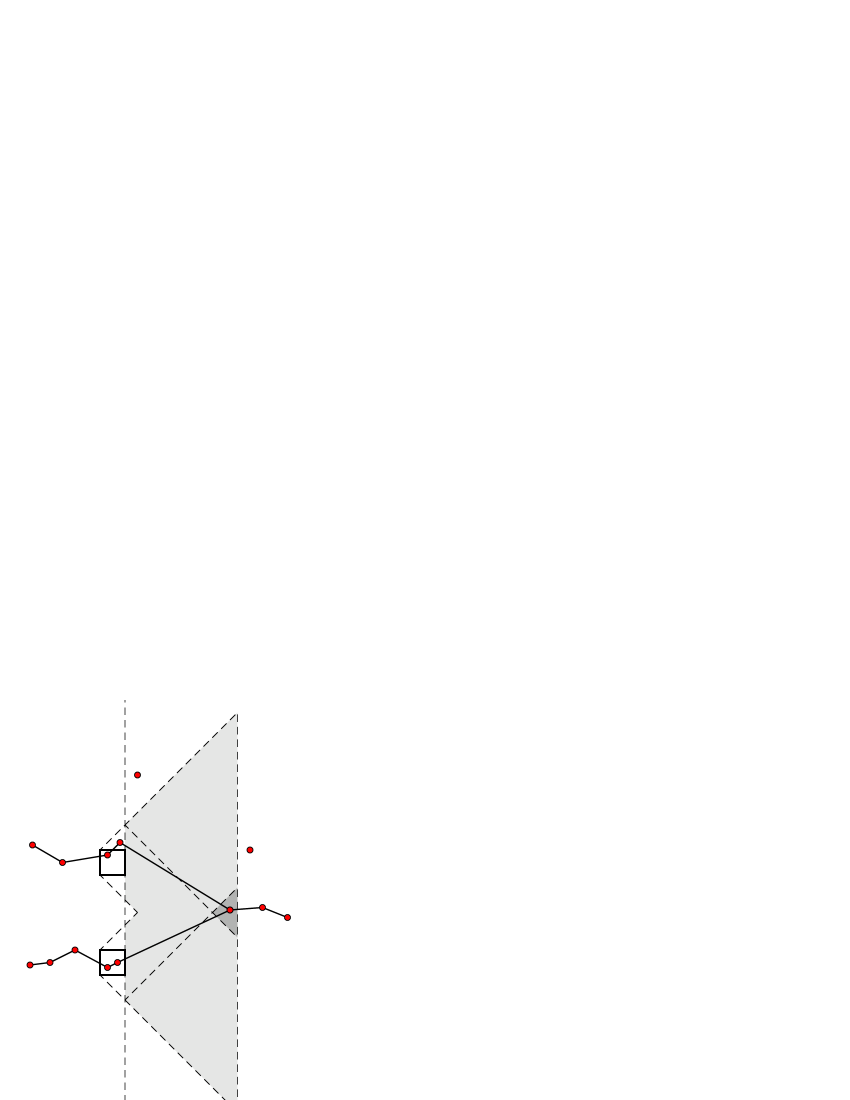
Figure 2: An event $B$ which forces coalescence of paths starting in two given cubes: the light gray region should be empty while the dark gray region should contain exactly one red point.

∎

5 Stable Matching

In this section we prove Theorems 5 and 6 as well as Proposition 9. We start with some relatively straightforward cases.

Proof of Theorem 5(ii).

Call a red point $x$ $t$-bad if $|{\cal M}(x)-x|>t$, and note that no two $t$-bad points may be within distance $t$ of each other, for they would form an unstable pair. Hence, using (4),

$$1\geq{\mathbb{E}}\#\big{\{}\text{$t$-bad red points in }B(0,\tfrac{t}{2})\big{\}}={\mathcal{L}}B(0,\tfrac{t}{2})\cdot{\mathbb{P}}^{*}(X>t).$$

∎

Proof of Theorem 6(ii) (case $d=1$).

Fix $t>0$. We say that a red point $x$ is $t$-bad if $|{\cal M}(x)-x|>t$. Let $W$ be the set of $t$-bad red points in the interval $[0,t]$, and denote the random variables

$$a=\min W;\quad b=\max W.$$

We claim that, provided $W\neq\emptyset$, every blue point in $[a,b]$ is matched to a red point in $[a,b]$. To prove this, suppose on the contrary that $x\in[a,b]$ is a blue point matched outside $[a,b]$. Without loss of generality suppose ${\cal M}(x)<a$. Then since $|{\cal M}(x)-x|>|a-x|$ and $|{\cal M}(a)-a|>t>|a-x|$, the pair $a,x$ would be unstable, a contradiction.

Since elements of $W$ are $t$-bad, they cannot be matched within $[a,b]\subseteq[0,t]$, so the above claim implies that ${\cal R}[a,b]-{\cal B}[a,b]\geq\#W$. Hence

$$\#W \leq\max_{[\alpha,\beta]\subseteq[0,t]}\Big{(}{\cal R}[\alpha,\beta]-{\cal B}[\alpha,\beta]\Big{)}$$

$$\leq\max_{z\in[0,t]}F(z)-\min_{z\in[0,t]}F(z),$$

where $F(z):={\cal R}[0,z]-{\cal B}[0,z]$. But $F$ is a continuous-time simple symmetric random walk, so (by e.g. [15, Proposition 13.13 and Theorem 14.6]) taking the expectation of the above inequality and using (4), we obtain

$$t\,{\mathbb{P}}^{*}(X>t)={\mathbb{E}}\#W\leq C\surd t$$

for a fixed constant $C\in(0,\infty)$. ∎

Proof of Theorem 6(ii) (case $d\geq 2$).

See Theorem 19 at the end of this section. ∎

To prove the lower bounds Theorems 5(i) and 6(i) we need the following simple properties of stable matchings and Poisson processes. The proofs are given after the statement of Lemma 18.

Lemma 15 (Stable partial matchings).

Let $U$ (respectively, $U,V$) be (disjoint) subset(s) of ${\mathbb{R}}^{d}$, and suppose that $U$ (respectively $U\cup V$) is discrete, non-equidistant, and has no descending chains. Then there is a unique stable partial matching of $U$ (respectively between $U$ and $V$), and it is produced by the iterated mutually closest matching algorithm described in the introduction. In the one-color case, there is at most one unmatched point, while in the two-color case, all unmatched points are of the same color.

It should be noted that stable marriage problems do not in general have unique solutions; see [8]. The key to uniqueness in our setting is that preferences are based on distance, and are therefore symmetric. Note also that some condition on $U$ (or $U\cup V$) is needed in order to guarantee existence and uniqueness of the stable matching. For example, in the one-color case with $d=1$, the set $U=\{0\}\cup\{3^{-n}:n\in{\mathbb{Z}}^{+}\}$ has no stable partial matching, while $U=\{\sum_{k=1}^{n}k^{-1}:n\in{\mathbb{Z}}^{+}\}$ has more than one.

Lemma 16 (Modifications for 1-color stable matching).

Let $U\subset{\mathbb{R}}^{d}$ be a discrete, non-equidistant set with no descending chains, and let $m$ be its unique stable partial matching.

• If $\{x,y\}\in m$ is a matched pair then $m\setminus\{\{x,y\}\}$ is the unique stable partial matching of $U\setminus\{x,y\}$.

• If $z\in{\mathbb{R}}^{d}\setminus U$ is such that $U\cup\{z\}$ is non-equidistant, and $|m(x)-x|<|z-x|$ for all $x\in U$, then $m$ is the unique stable partial matching of $U\cup\{z\}$ (in particular, $z$ is unmatched).

Lemma 17 (Monotonicity for 2-color stable matching).

Let $U,V,\{v^{\prime}\}$ $\subset{\mathbb{R}}^{d}$ be disjoint sets, and suppose that $U\cup V\cup\{v^{\prime}\}$ is discrete, non-equidistant, and has no descending chains. Let $m$ be the stable bipartite partial matching between $U$ and $V$, and let $m^{\prime}$ be the stable bipartite partial matching between $U$ and $V\cup\{v^{\prime}\}$. Then

$$|u-m^{\prime}(u)|\leq|u-m(u)|\quad\forall u\in U,$$

(where as usual $|x-m(x)|:=\infty$ if $x$ is unmatched).

Lemma 17 states that adding an extra blue point makes the matching no worse for red points. Such results are well-known for finite stable marriage problems – see e.g. [8, 16].

Lemma 18 (Modifications for Poisson process).

Let ${\cal R}$ be a homogeneous Poisson process.

• Let $U$ be a uniform random point in a set $S$ with ${\mathcal{L}}S\in(0,\infty)$, independent of ${\cal R}$. The law of the point process ${\cal R}+\delta_{U}$ obtained by adding a point at $U$ is absolutely continuous with respect to the law of ${\cal R}$.

• Let ${\cal F}$ be a simple point process whose support $[{\cal F}]$ is a.s. a random finite subset of $[{\cal R}]$. The law of the process ${\cal R}-{\cal F}$ obtained by removing the points of ${\cal F}$ is absolutely continuous with respect to the law of ${\cal R}$.

Proof of Lemma 15.

Consider the iterated mutually closest matching algorithm. Non-equidistance ensures that it is well-defined. We first claim that every pair matched by the algorithm are matched to each other in every stable partial matching. This is proved by induction on the stage of the algorithm: supposing the claim holds for all pairs matched so far, any remaining mutually closest pair cannot be matched to points removed earlier (by the inductive hypothesis) and they cannot be matched further away than each other (by stability).

Now consider the set $N$ of points left unmatched by the algorithm. We must show that these points are unmatched in every stable partial matching. This is clear if $\#N\leq 1$. Therefore, suppose that $\#N\geq 2$ and consider first the one-color case. Let $x_{0}\in N$, and let $x_{1}$ be the closest point to $x_{0}$ in $N\setminus\{x_{0}\}$, (which exists, by discreteness). Inductively, let $x_{n+1}$ be the point in $N\setminus\{x_{n}\}$ closest to $x_{n}$. Clearly, $|x_{n}-x_{n+1}|\geq|x_{n+1}-x_{n+2}|$ for all $n\in\mathbb{N}$. Since there is no descending chain, it follows that there is some first $m\in\mathbb{N}$ such that $x_{m+1}=x_{j}$ with $j\in\{0,1,\dots,m-1\}$. Because of non-equidistance, we must have $j=m-1$. But then $x_{m-1}$ and $x_{m}$ are mutually closest in $N$, which implies that they would have been matched by the algorithm right after all other points had been removed from $B\bigl{(}x_{m-1},|x_{m-1}-x_{m}|\bigr{)}\cup B\bigl{(}x_{m},|x_{m-1}-x_{m}|\bigr{)}$ (which would happen after a finite number of stages by discreteness). This contradicts $x_{m-1},x_{m}\in N$ and shows that $\#N\leq 1$.

In the two-color case, let $N_{U}$ be the unmatched points in $U$ and let $N_{V}$ be the unmatched points in $V$. If $N_{U}=\emptyset$, then clearly all points in $N_{V}$ are unmatched in every stable matching. The case $N_{V}=\emptyset$ is similar. If both $N_{U}$ and $N_{V}$ are nonempty, we choose $x_{0}\in N_{U}$ and inductively let $x_{2n+1}$ be the point in $N_{V}$ closest to $x_{2n}$ and let $x_{2n+2}$ be the point in $N_{U}$ closest to $x_{2n+1}$. The argument is then completed as in the one-color case. ∎

Proof of Proposition 9.

Apply Lemma 15 and consider the random process ${\cal N}$ of unmatched points in the unique stable partial matching - we must show that $[{\cal N}]$ is almost surely empty.

In the one-color case, the lemma implies that $\#[{\cal N}]\leq 1$. But if ${\cal N}$ has exactly one point with positive probability then (after conditioning on this event) its location would be a translation-invariant ${\mathbb{R}}^{d}$-valued random variable, which is impossible.

In the two-color case, the lemma implies that $[{\cal N}]$ must be empty, or consist entirely of red points or entirely of blue points. By ergodicity, one of these three possibilities must have probability 1. But Lemma 7 implies that the processes of unmatched red points and unmatched blue points have equal intensity, so the latter two possibilities are ruled out. ∎

Proof of Lemma 16.

By Lemma 15, we need only check that the claimed matching is stable. In (i) this is immediate, since any unstable pair would have been unstable in the original matching. Similarly in (ii), the given condition ensures that $z$ does not form an unstable pair with any $x\in U$. ∎

Proof of Lemma 17.

Suppose on the contrary that for some $u\in U$ we have $|u-m^{\prime}(u)|>|u-m(u)|$. In particular $m(u)\neq\infty$, so write $v:=m(u)\in V$. Stability of $(u,v)$ in $m^{\prime}$ implies $|v-m^{\prime}(v)|\leq|v-u|$, but $m^{\prime}(v)\neq u$ so non-equidistance implies that the previous inequality is strict; we write $u_{1}:=m^{\prime}(v)\in U$. Similarly, by stability of $(u_{1},v)$ in $m$ we have $|u_{1}-m(u_{1})|<|u_{1}-v|$; write $v_{1}:=m(u_{1})\in V$. Iterating this argument gives a descending chain $u,v,u_{1},v_{1},u_{2},v_{2},\ldots$. ∎

Proof of Lemma 18.

(i): It is elementary to check that the Radon-Nikodym derivative of the laws is $p(N-1)/p(N)$, where $N:={\cal R}(S)$, and $p(k)$ is the probability that $N=k$.

(ii): Let $A$ be some measurable set such that ${\mathbb{P}}(\mathcal{R}-\mathcal{F}\in A)>0$. We need to show that ${\mathbb{P}}(\mathcal{R}\in A)>0$. Since a.s. $[\mathcal{F}]$ is finite and $[\mathcal{R}]$ is discrete, there is a.s. a finite random set of balls with rational centers and radii such that $[\mathcal{F}]$ is the intersection of $[\mathcal{R}]$ with the union of these balls. Therefore, there is a deterministic finite union of open balls $W$ such that $\delta:={\mathbb{P}}(\mathcal{R}-\mathcal{F}\in A,\,[\mathcal{R}]\cap W=[\mathcal{F}])>0$. Let $\mathcal{R}_{1}$ denote the restriction of $\mathcal{R}$ to the complement of $W$, and let $A_{1}$ be the event that ${\mathbb{P}}\bigl{(}\mathcal{R}-\mathcal{F}\in A,\,[\mathcal{R}]\cap W=[\mathcal{F}]\bigm{|}\mathcal{R}_{1}\bigr{)}>\delta/2$. Note that ${\mathbb{P}}(A_{1})\geq\delta/2$. On the event $A_{1}$, with positive probability we have $\mathcal{R}-\mathcal{F}=\mathcal{R}_{1}$ and therefore $\mathcal{R}_{1}\in A$. But $A_{1}$ is $\sigma(\mathcal{R}_{1})$-measurable, so we must have $\mathcal{R}_{1}\in A$ a.s. on $A_{1}$. Since $\mathcal{R}_{1}$ and $\mathcal{R}(W)$ are independent, we deduce

$${\mathbb{P}}(\mathcal{R}\in A)\geq{\mathbb{P}}\big{(}A_{1},\,\mathcal{R}(W)=0\big{)}={\mathbb{P}}(A_{1})\,{\mathbb{P}}\big{(}\mathcal{R}(W)=0\big{)}>0.$$

∎

We now turn to the proofs of the lower bounds.

Proof of Theorem 5(i).

Let ${\cal M}$ be the one-color stable matching, and consider the random set

$$H=H({\cal R}):=\{x\in[{\cal R}]:|x-{\cal M}(x)|>|x|-1\}.$$ (18)

This is the set of red points that would prefer some red point in the unit ball $B(0,1)$ (if one were present in the correct location) over their current partners. We claim that

$${\mathbb{P}}(\#H=\infty)=1.$$ (19)

Once this is proved, we obtain the required result as follows, using (5) and Fubini’s theorem:

$$\infty={\mathbb{E}}\#H =\int_{{\mathbb{R}}^{d}}{\mathbb{P}}^{*}(X>|x|-1)\;dx$$

$$=\int_{0}^{\infty}{\mathbb{P}}^{*}(X+1>t)\,c\,t^{d-1}\;dt$$

$$=\frac{c}{d}\,{\mathbb{E}}^{*}\bigl{[}(X+1)^{d}\bigr{]},$$

hence ${\mathbb{E}}^{*}X^{d}=\infty$.

Returning to the claim (19), suppose on the contrary that $H$ is finite with positive probability. For each point configuration ${\cal R}$, construct a modified configuration $\widehat{{\cal R}}$ as follows:

• if $\#H<\infty$, remove all the points in $H\cup\{{\cal M}(x):x\in H\}$;

• add a uniformly random point in $B(0,1)$, independently of ${\cal R}$.

Using Lemma 18, the law of the random configuration $\widehat{{\cal R}}$ is absolutely continuous with respect to that of ${\cal R}$. Now by Lemma 16, whenever $\#H({\cal R})<\infty$, the stable partial matching of $[\widehat{{\cal R}}]$ has an unmatched point (the one added in (ii)), hence this happens with positive probability. Absolute continuity therefore implies that with positive probability the stable partial matching of $[{\cal R}]$ has an unmatched point, contradicting Proposition 9. ∎

Proof of Theorem 6(i).

Define the random set $H$ exactly as in (18) (now it is the set of red points which would prefer a blue point in $B(0,1)$). We will prove that ${\mathbb{P}}(\#H=\infty)=1$, whereupon the result follows as in the proof of Theorem 5(i).

Fix any $k<\infty$; we will prove that ${\mathbb{P}}(\#H\geq k)=1$. Let ${\cal B}^{\prime}$ be obtained from ${\cal B}$ by adding $k$ independent uniformly random points in $B(0,1)$. By Lemma 18(i), the law of $({\cal R},{\cal B}^{\prime})$ is absolutely continuous with respect to that of $({\cal R},{\cal B})$. Hence, by Proposition 9, almost surely all the $k$ added points are matched in the stable matching between $[{\cal R}]$ and $[{\cal B}^{\prime}]$. By Lemma 17, it follows that the partners of the added points were matched as far away or further in the stable matching with $[{\cal B}]$, so these partners lie in $H$, and thus $\#H\geq k$ as required. ∎

Remark.

As stated in the introduction, Theorem 6 holds also for the stable matching of heads (red) to tails (blue) on ${\mathbb{Z}}^{d}$ (given some tie-breaking rule). In order to adapt the proof of (i) to that setting, we claim that the set $H$ of red sites $v\in{\mathbb{Z}}^{d}$ which would prefer the origin to their current partner (if the origin was blue) must be infinite. Indeed, if $H$ is finite, then a contradiction is obtained by considering the configuration in which the sites in $H$ are recolored blue and the origin is colored blue.

Finally we prove the upper bound for the two-color stable matching in $d\geq 2$.

Theorem 19.

In the two-color stable matching of two independent Poisson processes of intensity 1 in ${\mathbb{R}}^{d}$, $d\geq 2$, we have

$${\mathbb{P}}^{*}(X>r)\leq C\,r^{-s}\,,$$ (20)

where $C=C(d)\in(0,1)$, and $s=s(d)$ is the unique solution in $(0,1)$ of the equation

$$2\,\omega_{d}\int_{1}^{2}(t-1)^{d-1}\,t^{-s}\,dt=\frac{\omega_{d-1}}{d-1}\int_{0}^{2}\bigl{(}1-(t/2)^{2}\bigr{)}^{\frac{d-1}{2}}\,t^{-s}\,dt\,,$$ (21)

and $\omega_{d}$ denotes the $(d-1)$-dimensional volume of the unit sphere in ${\mathbb{R}}^{d}$.

For $d=2$, (21) simplifies to

$$\sqrt{\pi}\,(2^{s}-2\,s)\,\Gamma\bigl{(}(2-s)/2\bigr{)}=\Gamma\bigl{(}(3-s)/2\bigr{)}\,,$$

and for general $d$ the integrals can be evaluated in terms of hypergeometric functions. The numerical values (rounded to the nearest $10^{-3}$) of $s$ at $d=2$, $3$, $10$ and $100$ are $0.496$, $0.449$, $0.339$ and $0.224$, respectively. It is not hard to see that $s_{d}\,\log d$ stays bounded away from $0$ and $\infty$ as $d\to\infty$.

Proof of Theorem 19.

Set $\alpha(r):={\mathbb{P}}^{*}(X>r)$. Fix some $R>0$ and consider the ball $B=B(0,R)$ of radius $R$ about $0$. Set

$$Y_{\cal R}:=\bigl{\{}x\in[{\cal R}]\cap B:|x-{\cal M}(x)|>R+|x|\bigr{\}},$$

and similarly

$$Y_{\cal B}:=\bigl{\{}x\in[{\cal B}]\cap B:|x-{\cal M}(x)|>R+|x|\bigr{\}}.$$

First, observe that if $x\in Y_{\cal R}$, then ${\cal M}(x)\notin B$. Next, note that if $x\in Y_{\cal R}$, then $x$ prefers any blue point in $B$ to its partner. Since the corresponding statement also holds for $Y_{\cal B}$, we have

$$\text{if $Y_{\cal R}\neq\emptyset$ then $Y_{\cal B}=\emptyset$}.$$ (22)

(This is the principal observation on which the proof rests.) Let $Q_{\cal B}$ denote the set of blue points in $B$ that are matched outside of $B$, and similarly for $Q_{\cal R}$.

Let $Z:={\cal R}(B)-{\cal B}(B)$, and note that $\#Q_{\cal R}-\#Q_{\cal B}=Z$. Therefore, $\#Y_{\cal R}\leq\#Q_{\cal B}+Z$, and (22) gives

$$\#Y_{\cal R}+\#Y_{\cal B}\leq\#Q_{\cal B}+Z^{+}.$$

Our bound will follow by taking the expectation of both sides of this inequality. Since ${\mathbb{E}}\#Y_{\cal R}={\mathbb{E}}\#Y_{\cal B}$ and ${\mathbb{E}}(Z^{+})\leq C\,R^{d/2}$ for some fixed constant $C=C_{d}$ (which may depend only on $d$), we get

$$2\,{\mathbb{E}}\#Y_{\cal R}\leq C\,R^{d/2}+{\mathbb{E}}\#Q_{\cal B}\,.$$ (23)

By (5), it is easy to express the left hand side in terms of $\alpha$, namely,

$${\mathbb{E}}\#Y_{\cal R} =\int_{B}\alpha(R+|x|)\,dx$$ (24)

$$=\omega_{d}\int_{0}^{R}\alpha(R+r)\,r^{d-1}\,dr=\omega_{d}\int_{R}^{2R}\alpha(r)\,(r-R)^{d-1}\,dr\,.$$

The proof will proceed by expressing ${\mathbb{E}}\#Q_{\cal B}$ in terms of $\alpha$ and using (23). Before embarking on the full argument we note the following simplified version which already gives a power law upper bound on $\alpha$. If a blue point in $B$ is matched outside $B$ then the length of its edge is at least its distance to the boundary of $B$, hence (5) gives

$${\mathbb{E}}\#Q_{\cal B} \leq\int_{B}\alpha(R-|x|)\,dx$$ (25)

$$=\omega_{d}\int_{0}^{R}\alpha(R-r)\,r^{d-1}\,dr=\omega_{d}\int_{0}^{R}\alpha(r)\,(R-r)^{d-1}\,dr\,.$$

Substituting (24) and (25) into (23) and using the fact that $\alpha$ is decreasing yields a bound for $\alpha(2R)$ in terms of $\alpha(r)$ for $r\in[0,R]$, and it is straightforward to deduce (by induction on $k$) that $\alpha(2^{k})\leq C^{\prime}(2^{k})^{-s^{\prime}}$ for some $C^{\prime}=C^{\prime}(d)\in(0,\infty)$ and $s^{\prime}=s^{\prime}(d)\in(0,1)$.

In order to get a better power we will instead use an exact expression for ${\mathbb{E}}\#Q_{\cal B}$, and analyze the resulting inequality more carefully. Denote the unit sphere $S^{d-1}:=\{z\in{\mathbb{R}}^{d}:|z|=1\}$. The intensity of the process of pairs $(x,u)\in{\mathbb{R}}^{d}\times S^{d-1}$ such that $x\in[{\cal B}]$, $|x-{\cal M}(x)|>r$ and $({\cal M}(x)-x)/|{\cal M}(x)-x|=u$ is precisely $\alpha(r)/\omega_{d}$. (That is, the expected number of such pairs in any set $A\subset{\mathbb{R}}^{d}\times S^{d-1}$ is $\alpha(r)/\omega_{d}$ times the volume of $A$.) For $x\in B$ and $u\in S^{d-1}$, let $q(x,u):=\inf\{t\geq 0:x+t\,u\notin B\}$, and fix some $u_{0}\in S^{d-1}$. Then

$${\mathbb{E}}\#Q_{\cal B}=\frac{1}{\omega_{d}}\int_{S^{d-1}}\int_{B}\alpha\bigl{(}q(x,u)\bigr{)}\,dx\,du=\int_{B}\alpha\bigl{(}q(x,u_{0})\bigr{)}\,dx\,,$$ (26)

where the last equality is a consequence of rotational symmetry. Let $L$ denote the orthogonal projection onto the subspace of ${\mathbb{R}}^{d}$ orthogonal to $u_{0}$; that is, $L\,z=z-(z\cdot u_{0})\,u_{0}$. For $x\in B$ define $f(x)=L\,x+q(x,u_{0})\,u_{0}$. Since $L\,f(x)=L\,x$ and $f(x+t\,u_{0})=f(x)-t\,u_{0}$, it follows by differentiation that $f$ is measure preserving. This allows us to use the substitution $z=f(x)$ and write

$${\mathbb{E}}\#Q_{\cal B}=\int_{f(B)}\alpha\bigl{(}z\cdot u_{0}\bigr{)}\,dz=\int_{0}^{2R}\mu_{d-1}\bigl{\{}z\in f(B):z\cdot u_{0}=r\bigr{\}}\,\alpha(r)\,dr\,,$$

where $\mu_{d-1}$ is $(d-1)$-dimensional Lebesgue measure and the last equality follows by Fubini. Now,

$$\mu_{d-1}\bigl{\{}z\in f(B):z\cdot u_{0}=r\bigr{\}}=\mu_{d-1}\bigl{\{}L\,x:x\in B,\,q(x,u_{0})=r\bigr{\}}\,.$$

Note that the set $\{L\,x:x\in B,\,q(x,u_{0})=r\bigr{\}}$ is precisely the set of sites $z\in L\,{\mathbb{R}}^{d}$ such that $z-(r/2)\,u_{0}\in B$, which is $\bigl{\{}z\in L\,{\mathbb{R}}^{d}:|z|<\sqrt{R^{2}-(r/2)^{2}}\bigr{\}}$. The $(d-1)$-volume of this set is just $\bigl{(}R^{2}-(r/2)^{2}\bigr{)}^{(d-1)/2}$ times the volume of the $(d-1)$-dimensional unit ball. Since the volume of the $(d-1)$-dimensional unit ball is $\omega_{d-1}/(d-1)$, we get

$${\mathbb{E}}\#Q_{\cal B}=\frac{\omega_{d-1}}{d-1}\,\int_{0}^{2R}\bigl{(}R^{2}-(r/2)^{2}\bigr{)}^{(d-1)/2}\,\alpha(r)\,dr\,.$$ (27)

Now, taking into account (23), (24) and (27), we obtain

$$\int_{0}^{\infty}g(r/R)\,\alpha(r)\,dr\leq C\,R^{1-d/2},$$

where

$$g(t):=2\,\omega_{d}\,{\mathbf{1}}_{[1,2]}(t)\,(t-1)^{d-1}-\frac{\omega_{d-1}}{d-1}\,{\mathbf{1}}_{[0,2]}(t)\,\bigl{(}1-(t/2)^{2}\bigr{)}^{\frac{d-1}{2}}.$$

This bound will be useful when $R$ is large. For $R$ small, we use the trivial estimate

$$\int_{0}^{\infty}g(r/R)\,\alpha(r)\,dr\leq\int_{0}^{\infty}g(r/R)\,dr\leq\int_{0}^{2R}\|g\|_{\infty}\,dr=2\,R\,\|g\|_{\infty}\,.$$

Combining these two estimates, we get

$$\int_{0}^{\infty}g(r/R)\,\alpha(r)\,dr\leq\min\{C\,R^{1-d/2},2\,R\,\|g\|_{\infty}\}\,.$$ (28)

We will get our desired bound on $\alpha$ by taking an appropriate average of (28) with respect to $R$.

Note that the set of $s$ satisfying $\int_{0}^{\infty}g(t)\,t^{-s}\,dt=0$ is precisely the set of $s$ satisfying (21). Observe that $g(t)$ is supported on $[0,2]$ and is continuous and monotone increasing there. Moreover, $g(0)<0<g(2)$. Therefore, there is some $s=s_{d}\in(-\infty,1)$ such that $\int_{0}^{\infty}g(t)\,t^{-s}\,dt=0$. We claim that $s$ is unique. Indeed, let $s^{\prime}<s$ and let $t_{0}$ be the unique solution of $g(t)=0$ in $(0,2)$. Then $t_{0}^{s^{\prime}-s}\,t^{-s^{\prime}}<t^{-s}$ precisely when $t<t_{0}$. Therefore $t_{0}^{s^{\prime}-s}\int_{0}^{\infty}g(t)\,t^{-s^{\prime}}\,dt>\int_{0}^{\infty}g(t)\,t^{-s}\,dt=0$, proving uniqueness. Next, we claim that $s>0$. Observe that if we replace $\alpha$ by $1$ we get the volume of $B$ (that is, $R^{d}\,\omega_{d}/d$) in (24) and (26). The algebraic manipulations within and following these equalities are valid for any measurable bounded function in place of $\alpha$. Therefore $\int_{0}^{\infty}g(t)\,dt=\mu_{d}(B(0,1))=\omega_{d}/d>0$, which implies $s>0$.

Since $\int_{0}^{\infty}g(t)\,t^{-s}\,dt=0$, a change of variables $t=r/\rho$ gives

$$\int_{0}^{\infty}g(r/\rho)\,\rho^{s-2}\,d\rho=0\,.$$ (29)

Set

$$G_{R}(r):=\int_{0}^{R}g(r/\rho)\,\rho^{s-2}\,d\rho\,.$$

We claim that $G_{R}(r)\geq 0$ for all $r>0$, and that

$$C_{0}:=\inf\bigl{\{}G_{R}(r)\,R^{1-s}:R>0,\,r\in[R/2,R]\bigr{\}}>0\,.$$

As before, let $t_{0}$ be the unique solution of $g(t)=0$ in $(0,2)$. If $r/R\geq t_{0}$, then $g(r/\rho)\geq 0$ for $\rho<R$, and hence $G_{R}(r)\geq 0$. On the other hand, if $r/R<t_{0}$, then $g(r/\rho)\leq 0$ for all $\rho>R$ and (29) gives $G_{R}(r)=-\int_{R}^{\infty}g(r/\rho)\,\rho^{s-2}\,d\rho\geq 0$. Since $g(t)>0$ for $t\in(t_{0},2)$ and $g(t)<0$ for $t\in(0,t_{0})$, the above reasoning actually gives $G_{R}(r)>0$ for $r\in(0,2\,R)$. Since $G_{R}$ is continuous, this implies $\inf_{r\in[1/2,1]}G_{1}(r)>0$. A change of variables gives $G_{R}(r)=R^{s-1}\,G_{1}(r/R)$, which now proves $C_{0}>0$.

From the monotonicity of $\alpha$, the definition of $C_{0}$ and from $G_{R}(r)\geq 0$, we now get

$$C_{0}\,R^{s}\,\alpha(R)/2\leq C_{0}\,R^{s-1}\int_{R/2}^{R}\alpha(r)\,dr\leq\int_{0}^{\infty}G_{R}(r)\,\alpha(r)\,dr\,.$$ (30)

Note that

$$\int_{0}^{R}\int_{0}^{\infty}\rho^{s-2}\,|g(r/\rho)|\,\alpha(r)\,dr\,d\rho\leq\int_{0}^{R}\int_{0}^{\infty}\rho^{s-2}\,\|g\|_{\infty}\,1_{r\leq 2\rho}\,dr\,d\rho<\infty\,.$$

Therefore, Fubini and (28) give

$$\int_{0}^{\infty}G_{R}(r)\,\alpha(r)\,dr =\int_{0}^{R}\left(\rho^{s-2}\,\int_{0}^{\infty}g(r/\rho)\,\alpha(r)\,dr\right)\,d\rho$$ (31)

$$\leq\int_{0}^{R}\rho^{s-2}\,\min\{C\,\rho^{1-d/2},2\,\rho\,\|g\|_{\infty}\}\,d\rho$$

$$\leq\int_{1}^{R}C\,\rho^{s-1-d/2}\,d\rho+2\,\|g\|_{\infty}\int_{0}^{1}\rho^{s-1}\,d\rho\,.$$

Since the right hand side is bounded in $R$ (this is where we use $d>1$), this and (30) imply (20). ∎

Remarks.

In order to adapt the proof of Theorem 19 to the stable allocation of Lebesgue to Poisson, we replace $\#Y_{\cal R}$ with the volume of sites $z\in B$ whose Poisson point is at distance greater than $R+|z|$, and replace $\#Y_{\cal B}$ with the sum over Poisson points $x\in B$ of the volume of $x$’s territory that is at distance greater than $R+|x|$. The mass transport principle easily shows that these two quantities have the same expectation. A similar remark applies to $\#Q_{\cal R}$ and $\#Q_{\cal B}$. This allows us to obtain the analog of (23).

To adapt the proof to the setting of a stable matching of heads to tails in ${\mathbb{Z}}^{d}$, we apply a uniform random translation in $[0,1)^{d}$, and then apply a random isometry preserving the origin. Then the law of the matching is invariant under isometries of ${\mathbb{R}}^{d}$, and the above proof applies.

Open Problems

• For the two-color stable matching of two independent Poisson processes, what is the correct power law for the tail behavior of $X$ in dimensions $d\geq 2$? We conjecture that ${\mathbb{E}}^{*}X^{\alpha}<\infty$ if and only if $\alpha<d/2$.

• Does there exist a translation-invariant matching of two independent Poisson processes in ${\mathbb{R}}^{2}$ such that the line segments connecting matched pairs do not cross?

Alexander E. Holroyd: holroyd(at)math.ubc.ca
University of British Columbia, 121-1984 Mathematics Rd,
Vancouver BC V6T 1Z2, Canada

Robin Pemantle: pemantle(at)math.upenn.edu
David Rittenhouse Laboratories, 209 S 33rd St,
Philadelphia PA 19104, USA

Yuval Peres: peres(at)microsoft.com
Oded Schramm:
Microsoft Research, One Microsoft Way,
Redmond WA 98052, USA

References

- [1] M. Ajtai, J. Komlós, and G. Tusnády. On optimal matchings. Combinatorica, 4(4):259–264, 1984.
- [2] K. S. Alexander. Percolation and minimal spanning forests in infinite graphs. Ann. Probab., 23(1):87–104, 1995.
- [3] D. Avis, B. Davis, and J. M. Steele. Probabilistic analysis of a greedy heuristic for euclidean matching. Probability in the Engineering and Information Sciences, 2:143–156, 1988.
- [4] I. Benjamini, R. Lyons, Y. Peres, and O. Schramm. Group-invariant percolation on graphs. Geom. Funct. Anal., 9(1):29–66, 1999.
- [5] S. Chatterjee, R. Peled, Y. Peres, and D. Romik. Gravitational allocation to Poisson points. Ann. Math., arXiv:math.PR/0611886. To appear.
- [6] P. A. Ferrari, C. Landim, and H. Thorisson. Poisson trees, succession lines and coalescing random walks. Ann. Inst. H. Poincaré Probab. Statist., 40(2):141–152, 2004.
- [7] A. Frieze, C. McDiarmid, and B. Reed. Greedy matching on the line. SIAM J. Comput., 19(4):666–672, 1990.
- [8] D. Gale and L. Shapley. College admissions and stability of marriage. Amer. Math. Monthly, 69(1):9–15, 1962.
- [9] O. Häggström and R. Meester. Nearest neighbor and hard sphere models in continuum percolation. Random Structures Algorithms, 9(3):295–315, 1996.
- [10] C. Hoffman, A. E. Holroyd, and Y. Peres. Tail bounds for the stable marriage of Poisson and Lebesgue. Canadian Journal of Mathematics, arXiv:math.PR/0507324. To appear.
- [11] C. Hoffman, A. E. Holroyd, and Y. Peres. A stable marriage of Poisson and Lebesgue. The Annals of Probability, 34(4):1241–1272, 2006, arXiv:math.PR/0505668.
- [12] A. E. Holroyd and T. M. Liggett. How to find an extra head: optimal random shifts of Bernoulli and Poisson random fields. Ann. Probab., 29(4):1405–1425, 2001.
- [13] A. E. Holroyd and Y. Peres. Trees and matchings from point processes. Electron. Comm. Probab., 8:17–27 (electronic), 2003.
- [14] A. E. Holroyd and Y. Peres. Extra heads and invariant allocations. Ann. Probab., 33(1):31–52, 2005.
- [15] O. Kallenberg. Foundations of modern probability. Probability and its Applications (New York). Springer-Verlag, New York, second edition, 2002.
- [16] D. E. Knuth. Stable marriage and its relation to other combinatorial problems, volume 10 of CRM Proceedings & Lecture Notes. American Mathematical Society, Providence, RI, 1997.
- [17] T. M. Liggett. Tagged particle distributions or how to choose a head at random. In In and out of equilibrium (Mambucaba, 2000), volume 51 of Progr. Probab., pages 133–162. Birkhäuser Boston, Boston, MA, 2002.
- [18] T. Soo. Translation-invariant matchings of coin-flips on . arXiv:math/0610334. Preprint.
- [19] M. Talagrand. The transportation cost from the uniform measure to the empirical measure in dimension . Ann. Probab., 22(2):919–959, 1994.
- [20] A. Timar. Invariant matchings of exponential tail on coin flips in . Preprint.