Energy of eigen-modes in magnetohydrodynamic flows of ideal fluids

Abstract

Analytical expression for energy of eigen-modes in magnetohydrodynamic flows of ideal fluids is obtained. It is shown that the energy of unstable modes is zero, while the energy of stable oscillatory modes (waves) can assume both positive and negative values. Negative energy waves always correspond to non-symmetric eigen-modes – modes that have a component of wave-vector along the equilibrium velocity. These results suggest that all non-symmetric instabilities in ideal MHD systems with flows are associated with coupling of positive and negative energy waves. As an example the energy of eigen-modes is calculated for incompressible conducting fluid rotating in axial magnetic field.

Energy consideration is of primary significance in stability analysis of different magnetohydrodynamic (MHD) systems. It is well known that the energy associated with the waves (purely oscillatory eigen-modes) may change its sign and become negative Fabrikant and Stepanyants (1998); Zhang and Lovelace (2005). The energy should be withdrawn from the system to let the negative energy wave be excited. So, a negative energy wave is a potential source of instability since no extra energy is needed to increase its intensity. Instability can arise, for example, if a negative energy wave is subject to external dissipation; then the subsequent removal of energy from the wave will cause it to grow. In a conservative system, the instability can occur due to the simultaneous excitation of positive and negative energy waves. In this case, energy is transferred from the negative energy wave to the positive energy wave, allowing both modes to grow and the total energy to remain constant. Waves having energies of various signs enable researches to explain different types of instabilities in fluid dynamics Lashmore-Davies (2005).

In the present paper we calculate the energy of the eigen-modes in ideal one-fluid MHD and show that all instabilities of non-symmetric eigen-modes in MHD systems with equilibrium flow are related to the coupling of negative and positive energy waves. Following Ref. Frieman and Rotenberg (1960), we consider linearized dynamics of displacement vector $\bf\xi$

$$\rho\frac{\partial^{2}\mbox{\boldmath$\bf\xi$}}{\partial t^{2}}+2\rho(\textbf{V}\cdot\nabla)\frac{\partial\mbox{\boldmath$\bf\xi$}}{\partial t}-\textbf{F}[\mbox{\boldmath$\bf\xi$}]=0,$$ (1)

where $\rho$ and V are stationary values of fluid density and velocity, respectively. The general form of linearized force operator $\textbf{F}[\mbox{\boldmath$\bf\xi$}]$ in ideal compressible MHD is

$$\textbf{F}[\mbox{\boldmath$\bf\xi$}] = -\rho(\textbf{V}\cdot\nabla)^{2}\mbox{\boldmath$\bf\xi$}+\rho(\mbox{\boldmath$\bf\xi$}\cdot\nabla)(\textbf{V}\cdot\nabla)\textbf{V}+$$

$$+ \nabla\cdot(\rho\mbox{\boldmath$\bf\xi$})(\textbf{V}\cdot\nabla)\textbf{V}-\nabla\delta P+$$

$$+ \frac{1}{4\pi}\,(\nabla\times\delta\textbf{B})\times\textbf{B}+\frac{1}{4\pi}\,(\nabla\times\textbf{B})\times\delta\textbf{B}.$$

Here, B is equilibrium magnetic field and

$$\delta\textbf{B}=\nabla\times(\mbox{\boldmath$\bf\xi$}\times\textbf{B})$$

is its perturbation. The perturbation of fluid pressure $\delta P$ can be specified by thermodynamic properties of the system. For example, if the process is adiabatic with adiabatic index $\gamma$ then

$$\delta P=-\mbox{\boldmath$\bf\xi$}\cdot\nabla P-\gamma P\nabla\cdot\mbox{\boldmath$\bf\xi$}.$$

In the case of incompressible MHD, such equation appears to be excessive, instead one has to impose the incompressibility condition $\nabla\cdot\mbox{\boldmath$\bf\xi$}=0$.

A number of formal properties of Eq. (1) can be established. Force operator $\textbf{F}[\mbox{\boldmath$\bf\xi$}]$ is Hermitian (self-adjoint) in the following sense,

$$\int\mbox{\boldmath$\bf\eta$}\cdot\textbf{F}[\mbox{\boldmath$\bf\xi$}]\,d^{3}\textbf{r}=\int\mbox{\boldmath$\bf\xi$}\cdot\textbf{F}[\mbox{\boldmath$\bf\eta$}]\,d^{3}\textbf{r},$$ (3)

while the second term in Eq. (1) is antisymmetric:

$$\int\rho\mbox{\boldmath$\bf\eta$}\cdot(\textbf{V}\cdot\nabla)\mbox{\boldmath$\bf\xi$}\,d^{3}\textbf{r}=-\int\rho\mbox{\boldmath$\bf\xi$}\cdot(\textbf{V}\cdot\nabla)\mbox{\boldmath$\bf\eta$}\,d^{3}\textbf{r}.$$ (4)

Integration in Eqs. (3) and (4) is performed over the fluid volume under the assumption that displacements on the boundary vanish.

In our subsequent discussion, the displacement vector $\bf\xi$ is supposed to be complex. In order to obtain the correct expression for energy of perturbations in this case, we multiply Eq. (1) by complex conjugate $\partial\mbox{\boldmath$\bf\xi$}^{*}/\partial t$ and integrate over the space:

$$\int\bigg{(}\rho\frac{\partial\mbox{\boldmath$\bf\xi$}^{*}}{\partial t}\cdot\frac{\partial^{2}\mbox{\boldmath$\bf\xi$}}{\partial t^{2}}+2\rho\frac{\partial\mbox{\boldmath$\bf\xi$}^{*}}{\partial t}\cdot(\textbf{V}\cdot\nabla)\frac{\partial\mbox{\boldmath$\bf\xi$}}{\partial t}-\frac{\partial\mbox{\boldmath$\bf\xi$}^{*}}{\partial t}\cdot\textbf{F}[\mbox{\boldmath$\bf\xi$}]\bigg{)}\,d^{3}\textbf{r}=0.$$

The complex conjugate of this equality is

$$\int\bigg{(}\rho\frac{\partial\mbox{\boldmath$\bf\xi$}}{\partial t}\cdot\frac{\partial^{2}\mbox{\boldmath$\bf\xi$}^{*}}{\partial t^{2}}+2\rho\frac{\partial\mbox{\boldmath$\bf\xi$}}{\partial t}\cdot(\textbf{V}\cdot\nabla)\frac{\partial\mbox{\boldmath$\bf\xi$}^{*}}{\partial t}-\frac{\partial\mbox{\boldmath$\bf\xi$}}{\partial t}\cdot\textbf{F}[\mbox{\boldmath$\bf\xi$}^{*}]\bigg{)}\,d^{3}\textbf{r}=0.$$

Summing up these two equations and using the properties (3), (4) we arrive at the energy conservation law in the form $\partial E/\partial t=0$, where

$$E=\frac{1}{2}\int\bigg{(}\rho\bigg{|}\frac{\partial\mbox{\boldmath$\bf\xi$}}{\partial t}\bigg{|}^{2}-\mbox{\boldmath$\bf\xi$}^{*}\cdot\textbf{F}[\mbox{\boldmath$\bf\xi$}]\bigg{)}\,d^{3}\textbf{r}.$$ (5)

As usual in mechanics, the total energy of the perturbations consists of kinetic part (first term) and of potential part (second term).

Since the equilibrium quantities have no time dependence, we look for a normal-mode solutions to Eq. (1) in the form

$$\mbox{\boldmath$\bf\xi$}(\textbf{r},t)=\hat{\mbox{\boldmath$\bf\xi$}}(\textbf{r})e^{-i\omega t}.$$ (6)

Then, the equation of motion (1) leads to eigen-value problem

$$\omega^{2}\rho\hat{\mbox{\boldmath$\bf\xi$}}+2i\omega\rho(\textbf{V}\cdot\nabla)\hat{\mbox{\boldmath$\bf\xi$}}+\textbf{F}[\hat{\mbox{\boldmath$\bf\xi$}}]=0.$$ (7)

Multiplying this equation by complex conjugate $\hat{\mbox{\boldmath$\bf\xi$}}^{*}$ and integrating over the fluid volume, we arrive at quadratic equation for eigen-frequency $\omega$,

$$A\,\omega^{2}-2B\,\omega-C=0,$$ (8)

with coefficients

$$A = \int\rho|\hat{\mbox{\boldmath$\bf\xi$}}|^{2}\,d^{3}\textbf{r}>0,$$

$$B = -\,i\int\rho\hat{\mbox{\boldmath$\bf\xi$}}^{*}\cdot(\textbf{V}\cdot\nabla)\hat{\mbox{\boldmath$\bf\xi$}}\,d^{3}\textbf{r},$$

$$C = -\int\hat{\mbox{\boldmath$\bf\xi$}}^{*}\textbf{F}[\hat{\mbox{\boldmath$\bf\xi$}}]\,d^{3}\textbf{r}.$$

Solving Eq. (8) we find

$$\omega_{1,2}=\frac{B\pm\sqrt{B^{2}+AC}}{A}.$$ (9)

This expression allows to determine eigen-frequency corresponding to known eigen-mode $\hat{\mbox{\boldmath$\bf\xi$}}$. Since all coefficients in Eq. (8) are real [for coefficients $C$ and $B$ it follows immediately from properties (3) and (4), respectively], the instability in the system is possible if and only if $B^{2}+AC<0$ for some eigen-mode.

Now we are able to determine the energy of the eigen-mode with eigen-frequency (9). Substituting (6) into expression (5) we obtain:

$$E=\frac{1}{2}\,(A\,|\,\omega|^{2}+C).$$ (10)

In the case of unstable mode, $B^{2}+AC<0$, so

$$|\,\omega_{1,2}|^{2}=-\frac{C}{A},$$

and the energy is

$$E_{1,2}=0.$$ (11)

For stable mode, $B^{2}+AC\geq 0$ and the energy is

$$E_{1,2} = \frac{\sqrt{B^{2}+AC}}{A}\,\bigg{(}\sqrt{B^{2}+AC}\pm B\bigg{)}=$$ (12)

$$= \pm\,\omega\,\sqrt{B^{2}+AC}.$$ (13)

Therefore, energy of stable eigen-mode changes the sign if its frequency changes the sign.

Depending on the system parameters different options are realized in the case of stable eigen-modes (Table 1). As one can see, there is an interval of parameters at which the waves with positive and negative energy coexist (option 2). One boundary of this interval corresponds to the stability threshold (option 1), the other – to change of sign of eigen-frequency $\omega_{2}$ (option 3). This result suggests that the instability in the ideal MHD system with flow can be associated with coupling of positive and negative energy waves.

We note here that all negative energy waves are non-symmetric modes, i.e., they have spatial dependence along the equilibrium flow, so, the coefficient $B\neq 0$. For symmetric modes or in the absence of flow we have $B=0$ and the energy is

$$E=\frac{1}{2}\,(|C|+C).$$

Therefore, energy of symmetric modes is never negative, and their stability can be investigated by use of energy principle Frieman and Rotenberg (1960). In a case of non-axisymmetric modes, the energy principle fails and special arrangements should be made to modify it (see, e.g., Ilgisonis and Khalzov (2005)).

Table 1: Eigen-frequencies $\omega_{\,1,2}$ and corresponding energies $E_{\,1,2}$ of stable eigen-modes for different values of coefficient $C$ ($B\geq 0$ is assumed for simplicity).

	$C$	$\omega_{1}$	$E_{1}$	$\omega_{2}$	$E_{2}$
1.	$-B^{2}/A$	+	0	+	$0$
2.	$(-B^{2}/A;~{}0)$	+	+	+	$-$
3.	$0$	+	+	0	$0$
4.	$(0;~{}\infty)$	+	+	$-$	+

In order to verify the above analytical results, we calculate the energy of eigen-modes of incompressible fluid rotating in homogenous transverse magnetic field $\textbf{B}=B\textbf{e}_{z}$. The equilibrium velocity profile used in our calculations corresponds to the electrically driven flow in circular channel and has a form

$$\textbf{V}=r\Omega(r)\textbf{e}_{\varphi},~{}~{}~{}\Omega(r)=\frac{\Omega_{1}r_{1}^{2}}{r^{2}}$$ (14)

in cylindrical system of coordinates $\{r,\varphi,z\}$. Here, $r_{1}$ and $r_{2}$ are inner and outer radii of the channel, respectively, and $\Omega_{1}$ is the angular velocity at $r_{1}$. This type of flow profile is used in new experimental device Velikhov et al. (2006) for laboratory testing of the so-called magnetorotational instability (MRI), which plays an important role in many astrophysical applications (see reviews Balbus and Hawley (1998); Balbus (2003)).

A detailed eigen-mode analysis of such flow has been performed in Ref. Khalzov et al. (2006). Assuming

$$\mbox{\boldmath$\bf\xi$}(\textbf{r},t)=\mbox{\boldmath$\bf\xi$}(r)e^{-i\omega t+im\varphi+ik_{z}z}$$

one obtains eigen-value problem

$$(\bar{\omega}^{2}-\omega_{A}^{2})\mbox{\boldmath$\bf\xi$}+2i\Omega\bar{\omega}(\xi_{r}\textbf{e}_{\varphi}-\xi_{\varphi}\textbf{e}_{r})-\frac{\partial\Omega^{2}}{\partial r}\,r\xi_{r}\textbf{e}_{r}=\nabla\delta\Pi,$$

$$\frac{1}{r}\frac{\partial(r\xi_{r})}{\partial r}+\frac{im}{r}\,\xi_{\varphi}+ik_{z}\xi_{z}=0$$ (15)

with boundary conditions

$$\xi_{r}(r_{1})=\xi_{r}(r_{2})=0,$$ (16)

where

$$\omega_{A}=\frac{k_{z}B}{\sqrt{4\pi\rho}}$$

is Alfven frequency,

$$\bar{\omega}=\omega-m\Omega$$

is ”shifted” eigen-frequency and $\delta\Pi$ is perturbation of the total normalized pressure,

$$\Pi=\frac{P}{\rho}+\frac{\textbf{B}^{2}}{4\pi\rho}.$$

A general expression for energy of perturbations (5) for this system reads

$$E=\frac{\rho}{2}\int\bigg{(}\bigg{|}\frac{\partial\mbox{\boldmath$\bf\xi$}}{\partial t}\bigg{|}^{2} + (\omega_{A}^{2}-m^{2}\Omega^{2})|\mbox{\boldmath$\bf\xi$}|^{2}+r\frac{\partial\Omega^{2}}{\partial r}\,|\,\xi_{r}|^{2}+$$ (17)

$$+ 2im\Omega^{2}(\xi_{r}\xi^{*}_{\varphi}-\xi^{*}_{r}\xi_{\varphi})\bigg{)}\,d^{3}\textbf{r}.$$

Substituting $\bf\xi$ from the eigen-value problem (Energy of eigen-modes in magnetohydrodynamic flows of ideal fluids), (16) we find the energy of stable mode with frequency $\omega$:

$$E = \pi\rho h\omega\int\limits_{r_{1}}^{r_{2}}r\bigg{\{}\bar{\omega}\bigg{[}\xi_{r}^{2}+\frac{1}{m^{2}+k_{z}^{2}r^{2}}\bigg{(}\frac{\partial(r\xi_{r})}{\partial r}\bigg{)}^{2}+$$

$$+ \frac{4k_{z}^{2}r^{2}\Omega^{2}\omega_{A}^{2}\xi_{r}^{2}}{(\omega_{A}^{2}-\bar{\omega}^{2})^{2}(m^{2}+k_{z}^{2}r^{2})}\bigg{]}+\frac{2m\Omega\xi_{r}}{m^{2}+k_{z}^{2}r^{2}}\frac{\partial(r\xi_{r})}{\partial r}\bigg{\}}\,dr,$$

where $h$ is the height of the channel. For axisymmetric eigen-modes with $m=0$ this expression is reduced to

$$E=\pi\rho h\omega^{2}\int\limits_{r_{1}}^{r_{2}}\bigg{[}\xi_{r}^{2}+\frac{1}{k_{z}^{2}r^{2}}\bigg{(}\frac{\partial(r\xi_{r})}{\partial r}\bigg{)}^{2}+\frac{4\Omega^{2}\omega_{A}^{2}\xi_{r}^{2}}{(\omega_{A}^{2}-\omega^{2})^{2}}\bigg{]}r\,dr.$$

Therefore, the energy of axisymmetric eigen-modes is always positive if $\omega\neq 0$. Formally, this case is described by (12) with coefficient $B=0$.

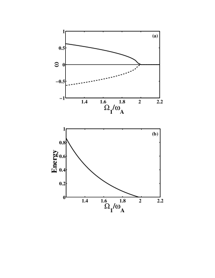
Figure 1: Calculated dependence of eigen-frequency (a) and energy (b) on ratio $\Omega_{1}/\omega_{A}$ for two most unstable eigen-modes with azimuthal number $m=0$. Energy is given in arbitrary units.

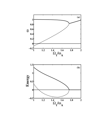
Figure 2: Calculated dependence of eigen-frequency (a) and energy (b) on ratio $\Omega_{1}/\omega_{A}$ for two most unstable eigen-modes with azimuthal number $m=1$. Energy is given in arbitrary units.

In Figs. 1, 2 the calculated dependencies of frequency and energy for two potentially unstable eigen-modes on the parameter $\Omega_{1}/\omega_{A}$ are shown. In the axisymmetric case ($m=0$), both branches of energy are positive and coincident (Fig. 1b). The merging point in Fig. 1a corresponds to $\Omega_{1}/\omega_{A}\approx 2.0$ which is the threshold of magnetorotational instability for $m=0$. The nature of axisymmetric MRI is not related to the subject of negative energy waves and can be explained by the mechanism similar to one of Raleigh-Taylor instability Velikhov (1959).

For $m=1$ the behavior of both energy curves in Fig. 2b is completely described by Eq. (12). The MRI threshold in this case is $\Omega_{1}/\omega_{A}\approx 1.7$. When $1.1\lesssim\Omega_{1}/\omega_{A}\lesssim 1.7$ the positive and negative energy waves can coexist in the system. At $\Omega_{1}/\omega_{A}\approx 1.1$ the frequency $\omega_{2}$ changes the sign (Fig. 2a, dashed line), so both energy branches become positive.

It should be noted that merging points in Figs. 1 and 2 determine the magnetorotational instability threshold. In the flow given by (14) this threshold decreases with azimuthal number $m$, as discussed in Ref. Khalzov et al. (2006). For large $m$ it approaches the asymptote

$$\frac{\Omega_{1}}{\omega_{A}}=\frac{2}{m(1-r_{1}^{2}/r_{2}^{2})}.$$ (19)

The calculated dependence of MRI threshold on small $m$ is presented in Fig. 3.

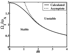
Figure 3: Calculated dependence of magnetorotational instability threshold on azimuthal mode number $m$ (solid line) and its asymptote for large $m$ (dashed line).

In conclusion, we have shown that all non-symmetric MHD instabilities in ideal fluids with flows can be explained as a coupling of originally stable positive and negative energy waves. These results are supported by calculations of frequencies and energies of eigen-modes in the flow that can be unstable with respect to magnetorotational instability.

This work is supported in part by NSERC Canada.

References

Fabrikant and Stepanyants (1998)
A. L. Fabrikant
and Y. A.
Stepanyants, Propagation of waves in
shear flows (World Scientific, 1998).
Zhang and Lovelace (2005)
L. Zhang and
R. V. E. Lovelace,
Astrophys. and Space Science
300, 395 (2005).
Lashmore-Davies (2005)
C. N. Lashmore-Davies,
J. Plasma Phys. 71,
101 (2005).
Frieman and Rotenberg (1960)
E. Frieman and
M. Rotenberg,
Rev. Mod. Phys. 32,
898 (1960).
Ilgisonis and Khalzov (2005)
V. I. Ilgisonis
and I. V.
Khalzov, JETP Letters
82, 570 (2005).
Velikhov et al. (2006)
E. P. Velikhov,
A. A. Ivanov,
S. V. Zakharov,
V. S. Zakharov,
A. O. Livadny,
and K. S.
Serebrennikov, Physics Letters A
358, 216 (2006).
Balbus and Hawley (1998)
S. A. Balbus and
J. F. Hawley,
Rev. Mod. Phys. 70,
1 (1998).
Balbus (2003)
S. A. Balbus,
Annu. Rev. Astron. Astrophys.
41, 555 (2003).
Khalzov et al. (2006)
I. V. Khalzov,
V. I. Ilgisonis,
A. I. Smolyakov,
and E. P.
Velikhov, Phys. Fluids
18, 124107 (2006).
Velikhov (1959)
E. P. Velikhov,
Sov. Phys. JETP 9,
995 (1959).