Abstract

We study four different approximations for finding the profile of discrete solitons in the one-dimensional Discrete Nonlinear Schrödinger (DNLS) Equation. Three of them are discrete approximations (namely, a variational approach, an approximation to homoclinic orbits and a Green-function approach), and the other one is a quasi-continuum approximation. All the results are compared with numerical computations.

1 Introduction

Since the 1960’s, a large number of works has focused on the properties of solitons in the Nonlinear Schrödinger (NLS) Equation [1]. As it is well known, the one-dimensional NLS equation is integrable. Two of the most important discretizations of this equation admit discrete solitons. One of these discretizations is known as the Ablowitz-Ladik equation [2], which is also integrable. On the contrary, the other important discretization, known as the Discrete Nonlinear Schrödinger (DNLS) equation, is not integrable, and discrete soliton solutions must be calculated numerically. The DNLS equation has many interesting mathematical properties and physical applications [3]. The DNLS equation models, among others, an array of nonlinear-optical waveguides [4], that was originally implemented in an experiment as a set of parallel ribs made of a semiconductor material (AlGaAs) and mounted on a common substrate [5]. It was predicted [6] that the DNLS equation may also serve as a model for Bose-Einstein condensates (BECs) trapped in a strong optical lattice, which was confirmed by experiments [7]. In addition to the direct physical realizations in terms of nonlinear optics and BECs, the DNLS equation appears as an envelope equation for a large class of nonlinear lattices (for references, see [9], Section 2.4). Accordingly, the solitons known in the DNLS equation represent intrinsic localized modes investigated in such chains experimentally [10] and theoretically [11, 12]. In this context, previous formal derivations of the DNLS equation have been mathematically justified for small amplitude time-periodic solutions in references [13].

In this paper we will consider fundamental solitons, which are of two types: Sievers-Takeno (ST) modes, which are site-centered [14], and Page (P) modes, which are bond-centered [15] (see also Fig. 1). They can also be seen, respectively, as discrete solitons with a single excited site, or two adjacent excited site with the same amplitude. The DNLS equation is given by

$$i\dot{u}_{n}+\varepsilon\left(u_{n+1}+u_{n-1}-2u_{n}\right)+\gamma|u_{n}|^{2}u_{n}=0,$$ (1)

where $u_{n}(t)$ are the lattice dynamical variables, the overdot stands for the time derivative, $\epsilon>0$ is the lattice coupling constant and $\gamma$ a nonlinear parameter. We look for solutions of frequency $\Lambda$ having the form $u_{n}(t)=e^{i\Lambda t}v_{n}$. Their envelope $v_{n}$ satisfies

$$-\Lambda v_{n}+\varepsilon\left(v_{n+1}+v_{n-1}-2v_{n}\right)+\gamma|v_{n}|^{2}v_{n}=0.$$ (2)

Throughout this paper, we assume $\gamma\varepsilon>0$ and choose $\gamma=\varepsilon=1$ without loss of generality, as Eq. (2) can be rescaled. We also look for unstaggered solutions, for which, $\Lambda>0$ (staggered solutions with $\Lambda<0$ can be mapped to the former upon a suitable staggering transformation $\tilde{v}_{n}=(-1)^{n}v_{n}$). Furthermore, we restrict to real solutions of (2), which yield (up to multiplication by $\exp{i\theta}$) all the homoclinic solutions of (2) [16]. Homoclinic solutions of (2) can be found numerically using methods based on the anti-continuous limit [11] and have been studied in detail (first of all, in one-dimensional models, but many results have been also obtained for two- and three-dimensional DNLS lattices) [3].

The aim of this paper is to compare four different analytical approximations of the profiles of ST- and P-modes together with the exact numerical solutions. These analytical approximations are of four types: one of variational kind, another one based on a polynomial approximation of stable and unstable manifolds for the DNLS map, another one based on a Green-function method, and, finally, a quasi-continuum approach.

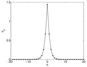
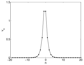
Figure 1: Discrete soliton profiles with $\Lambda=\varepsilon=\gamma=1$. Left panel corresponds to a ST-mode, and right panel, to a P-mode.

2 Discrete approximations

2.1 The variational approximation

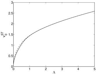
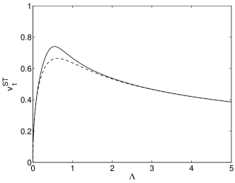
Figure 2: Dependence, for ST-modes, of $v_{0}$ (left panel) and $v_{1}$ (right panel) with respect to $\Lambda$. Full lines correspond to the exact numerical solution and dashed lines to the variational approximation.

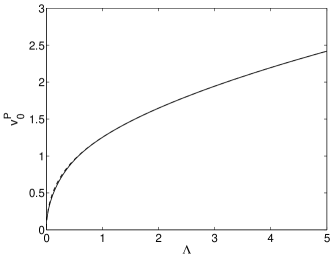
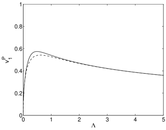
Figure 3: Dependence, for P-modes, of $v_{0}$ (left panel) and $v_{1}$ (right panel) with respect to $\Lambda$. Full lines correspond to the exact numerical solution while dashed lines correspond to the variational approximation.

Equation (2) can be derived as the Euler-Lagrange equation for the Lagrangian

$$L_{\mathrm{eff}}=\sum_{n=-\infty}^{+\infty}\left[(v_{n+1}+v_{n-1})v_{n}-(\Lambda+2)v_{n}^{2}+\frac{1}{2}v_{n}^{4}\right].$$ (3)

The VA for fundamental discrete solutions, elaborated in Ref. [17] (see also Ref. [18]) was based on the simple exponential ansatz ,

$$v^{ST}_{n}=A_{1}e^{-a_{1}|n|},\qquad v^{P}_{n}=A_{2}e^{-a_{2}|n+1/2|},$$ (4)

where $v^{ST}_{n}$ denotes ST-modes, while $v^{P}_{n}$ is for P-modes, with variational parameters $A_{1}$, $A_{2}$, $a_{1}$ and $a_{2}$ (which determine the amplitude and inverse size of the soliton). Then, substituting the ansatz in the Lagrangian, one can perform the summation explicitly, which yields the effective Lagrangian,

$$L^{ST}_{\mathrm{eff}}=\mathcal{N}_{1}(2\mathrm{sech}\ a_{1}-\Lambda-2)+\frac{\mathcal{N}_{1}^{2}\tanh^{2}a_{1}}{2\tanh 2a_{1}},\quad L^{P}_{\mathrm{eff}}=\mathcal{N}_{2}\left(\frac{2(1-\cosh a_{2})}{\sinh a_{2}+\cosh a_{2}}-\Lambda\right)+\frac{\mathcal{N}_{2}^{2}}{4}\tanh a_{2}$$ (5)

The norm of the ansatz (4), which appears in Eq. (5), is given by $\mathcal{N}\equiv\sum_{n=-\infty}^{+\infty}v_{n}^{2}$. In particular, for the ST- and P-modes,

$$\mathcal{N}_{1}=A_{1}^{2}\coth a_{1},\qquad\mathcal{N}_{2}=A_{2}^{2}/\sinh a_{2}.$$ (6)

The Lagrangian (5) gives rise to the variational equations, $\partial L^{ST}_{\mathrm{eff}}/\partial\mathcal{N}_{1}=\partial L^{ST}_{\mathrm{eff}}/\partial a_{1}=0$, and $\partial L^{P}_{\mathrm{eff}}/\partial\mathcal{N}_{2}=\partial L^{P}_{\mathrm{eff}}/\partial a_{2}=0$, which constitute the basis of the VA [19]. These predict relations between the norm, frequency, and width of the discrete solitons within the framework of the VA, namely

$$\mathcal{N}_{1}=\frac{4\cosh a_{1}\sinh^{2}2a_{1}}{\sinh 4a_{1}-\sinh 2a_{1}},\quad\mathcal{N}_{2}=\frac{8(1-\cosh a_{2}+\sinh a_{2})\cosh^{2}a_{2}}{\sinh a_{2}+\cosh a_{2}}$$ (7)

$$\Lambda=2(\mathrm{sech}\ a_{1}-1)+\mathcal{N}_{1}\frac{\tanh^{2}a_{1}}{\tanh 2a_{1}},\quad\Lambda=\frac{2(1-\cosh a_{2})}{\sinh a_{2}+\cosh a_{2}}+\frac{1}{2}\mathcal{N}_{2}\tanh a_{2}.$$ (8)

These analytical predictions, implicitly relating $\mathcal{N}$ and $\Lambda$ through their parametric dependence on the inverse width parameter $a$, will be compared with numerical findings below. In Figs. 2 and 3, we compare the approximate and exact values of the highest amplitude site and the second-highest amplitude sites (i.e. $v_{0}$ and $v_{1}$, which can be easily calculated from (7) once $\mathcal{N}$ and $a$ are known) with respect to $\Lambda$ for both ST- and P-modes.We can observe that the variational approach captures the exact asymptotic behavior as $\Lambda\rightarrow+\infty$. Indeed as $a_{1}\rightarrow+\infty$ in approximation (4) one obtains $\Lambda\sim\mathcal{N}_{1}\sim e^{a_{1}}$ and $A_{1}\sim\sqrt{\mathcal{N}_{1}}\sim\sqrt{\Lambda}$. Thus $v^{ST}_{0}\sim\sqrt{\Lambda}$ as $\Lambda\rightarrow+\infty$ which is indeed the asymptotic behavior of the exact ST-mode. On the contrary, the variational approximation errs by a small multiplicative factor ($\frac{2}{\sqrt{3}}\sim 1.1$) as $\Lambda\rightarrow 0$ (i.e., effectively approaching the continuum limit). This can be seen taking the limit $a_{1}\rightarrow 0$ in approximation (4). One has $\mathcal{N}_{1}\sim 8a_{1}$, $\Lambda\sim-a_{1}^{2}+\frac{a_{1}}{2}\mathcal{N}_{1}\sim 3a_{1}^{2}$ and $A_{1}\sim 2\sqrt{2}a_{1}\sim\frac{2}{\sqrt{3}}\sqrt{2\Lambda}$, while the amplitude of the continuum hyperbolic secant soliton of the integrable NLS is $A=\sqrt{2\Lambda}$ [see also below]. Notice that the P-mode also has the same $\Lambda\rightarrow 0$ limit (and therefore errs by the same factor).

2.2 The homoclinic orbit approximation

2.2.1 The DNLS map

The difference equation (2) can be recast as a two-dimensional real map by defining $y_{n}=v_{n}$ and $x_{n}=v_{n-1}$ [20, 21, 22, 18, 16]:

$$\left\{\begin{array}[]{l}x_{n+1}=y_{n}\\ y_{n+1}=-y_{n}^{3}+(\Lambda+2)y_{n}-x_{n}.\\ \end{array}\right.$$ (9)

For $\Lambda>0$, the origin $x_{n}=y_{n}=0$ is hyperbolic and a saddle point, which is checked upon linearization of the map around this point. Consequently, there exists a 1-d stable and a 1-d unstable manifolds emanating from the origin in two directions given by $y=\lambda_{\pm}x$, with

$$\lambda_{\pm}=\frac{(2+\Lambda)\pm\sqrt{\Lambda(\Lambda+4)}}{2}.$$ (10)

The eigenvalues $\lambda_{\pm}$ satisfy $\lambda^{2}-(\Lambda+2)\lambda+1=0$ and $\lambda_{+}=\lambda_{-}^{-1}>1$. The stable and unstable manifolds are invariant under inversion as it is the case for eq. (9). Moreover, they are exchanged by the symmetry $(x,y)\rightarrowtail(y,x)$ (this is due to the fact that the map (9) is reversible; see e.g. [16] for more details). Due to the non-integrability of the DNLS equation, these manifolds intersect in general transversally, yielding the existence of an infinity of homoclinic orbits (see Figs. 4 and 5). Each of their intersections corresponds to a localized solution, which can be a fundamental soliton or a multi-peaked one. Fundamental solitons, the solutions we are interested in, correspond to the primary intersections points, i.e. those emanating from the first homoclinic windings. Each intersection point defines an initial condition $(x_{0},y_{0})$, that is, $(v_{-1},v_{0})$, and the rest of the points composing the soliton are determined by application of the map.

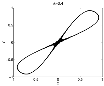
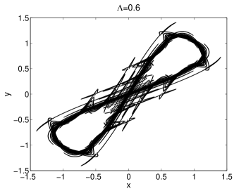
Figure 4: Homoclinic tangles for $\Lambda=0.4$, $\Lambda=0.6$.

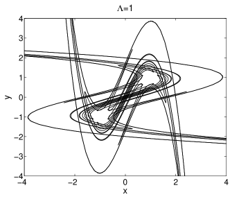
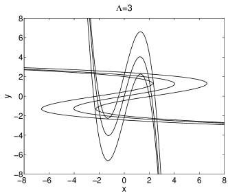
Figure 5: Homoclinic tangles for $\Lambda=1$ and $\Lambda=3$.

2.2.2 The polynomial approximation to the unstable manifold

The first windings of the stable and unstable manifolds can be approximated by third order polynomials. Actually, only one of them is necessary to be determined, as the other one is determined taking into account the symmetry $x\leftrightarrow y$. We proceed then to approximate the local unstable manifold $W^{u}_{\mathrm{loc}}(0)$. Taking into account its invariance under inversion, it can be locally written as a graph $y=f(x)=\lambda x-\alpha x^{3}+O(|x|^{5})$ with $\lambda\equiv\lambda_{+}$ given by (10). For $x\approx 0$, the image of $(x,f(x))$ under the map (9) also belongs to $W^{u}_{\mathrm{loc}}(0)$, thus $-f(x)^{3}+(\Lambda+2)f(x)-x=f(f(x))\ \forall x\approx 0$. This yields $[\lambda^{3}+\alpha(\Lambda+2-\lambda-\lambda^{3})]x^{3}+O(|x|^{5})=0,\ \forall x\approx 0$. Hence $\alpha=-\lambda^{3}/(\Lambda+2-\lambda-\lambda^{3})=\lambda^{4}/(\lambda^{4}-1)$. The local unstable manifold is approximated at order 3 by

$$W^{u}:y=\lambda x-\frac{\lambda^{4}}{\lambda^{4}-1}x^{3},$$ (11)

and, by symmetry, the stable manifold is approximated by:

$$W^{s}:x=\lambda y-\frac{\lambda^{4}}{\lambda^{4}-1}y^{3}.$$ (12)

In Fig. 6, the numerical and approximated unstable manifolds for $\Lambda=1$ and $\Lambda=3$ are compared. It can be observed that the fit is better when $\Lambda$ increases. The approximation breaks down for small $\Lambda$ because the origin is not a hyperbolic fixed point for $\Lambda=0$.

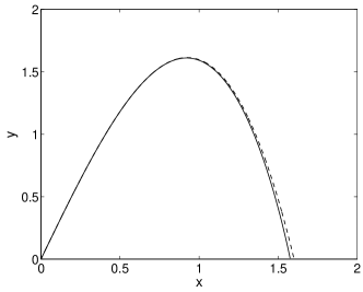
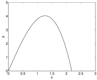
Figure 6: Numerical exact unstable manifold (full line) and its approximation by Eq. (11) (dashed line) for $\Lambda=1$ (left panel) and $\Lambda=3$ (right panel). The fit is so accurate in the latter that both curves are superimposed.

Figure 7: (Left panel) Approximated stable and unstable manifolds for $\Lambda=2$ showing the main intersections. (Right panel) Pitchfork bifurcation arising in the homoclinic approximation when $\Lambda$ is varied. ST-modes (full lines) bifurcate with the P-mode (dashed line) at $\Lambda=0.5$.

2.2.3 Approximate solutions via approximate invariant manifolds

Once an analytical form of the unstable and stable manifold is found, discrete solitons profiles (or, concretely, $v_{0}$ and $v_{-1}$) can be determined as the intersection of both manifolds. The polynomial form of (11) is not sufficient in practice to obtain good approximations of the whole soliton profile, due to sensitivity under initial conditions. However, it provides a good approximation near the soliton center. Some intersections of $W^{s}$ and $W^{u}$ can be approximated by:

$$x=\lambda\left(\lambda x-\frac{\lambda^{4}}{\lambda^{4}-1}x^{3}\right)-\frac{\lambda^{4}}{\lambda^{4}-1}\left(\lambda x-\frac{\lambda^{4}}{\lambda^{4}-1}x^{3}\right)^{3}.$$ (13)

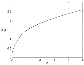
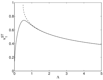
Figure 8: Same as Fig. 2 but with dashed lines corresponding to approximation (14).

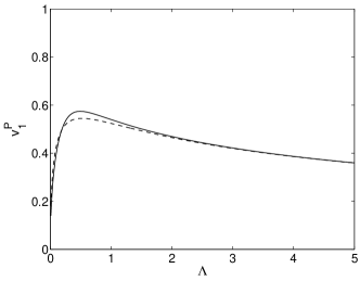
Figure 9: Same as Fig. 3 but with dashed lines corresponding to approximation (15).

This equation has nine solutions (see Fig. 7a). One of them ($x=0$), corresponds to the origin. Once this solution is eliminated, the reminder equation is a bi-quartic one. Thus, if $x=\xi$ is a solution of (13), $x=-\xi$ is also a solution: this is due to the fact that $\pm v_{n}$ is a solution of (2). Solutions $x=\xi_{1}$, $x=\xi_{2}$, $x=\xi_{0}$ and $x=\xi_{3}$ in Fig. 7 correspond to the positive solutions of (13). The point $x=\xi_{0}$ is in the bisectrix of the first quadrant and corresponds to the P-mode (i.e. $v_{0}^{P}=\xi_{0}$), and the point $x=\xi_{3}$ lies in the bisectrix of the fourth quadrant and corresponds to a twisted mode (i.e. a discrete soliton with two adjacent excited sites with the same amplitude and opposite sign). Setting $y(\xi_{0})=\xi_{0}$ and $y(\xi_{3})=-\xi_{3}$ in (11), one obtains $\xi_{0}=\lambda^{-2}\sqrt{(\lambda-1)(\lambda^{4}-1)}$, $\xi_{3}=\lambda^{-2}\sqrt{(\lambda+1)(\lambda^{4}-1)}$.

Upon elimination of the roots $x=\xi_{0}$ and $x=\xi_{3}$ from (13), $\xi_{1}$ and $\xi_{2}$ can be calculated as solutions of a quadratic equation. Thus,

$$\xi_{1}=\lambda^{-2}\sqrt{(\lambda^{4}-1)(\lambda-\sqrt{\lambda^{2}-4})/2},\quad\xi_{2}=\lambda^{-2}\sqrt{(\lambda^{4}-1)(\lambda+\sqrt{\lambda^{2}-4})/2}.$$ (14)

These solutions are related with the ST-mode as $v_{0}^{ST}=\xi_{2}$ and $v_{1}^{ST}=\xi_{1}$. On the other hand, for the P-mode, $v_{0}^{P}=\xi_{0}$, and, $v_{1}^{P}$ should be determined by application of the map (9). This yields

$$v_{0}^{P}=\lambda^{-2}\sqrt{(\lambda-1)(\lambda^{4}-1)},\quad v_{1}^{P}=\lambda^{-6}(\lambda^{3}+\lambda-1)\sqrt{(\lambda-1)(\lambda^{4}-1)}.$$ (15)

In Figs. 8 and 9, the values of $v_{0}$ and $v_{1}$ obtained through the homoclinic approximation are represented versus $\Lambda$ and compared with the exact numerical results. It can be observed that, for ST-modes, no approximate solutions exist for $\Lambda<0.5$. For $\Lambda=1/2$ (i.e. $\lambda=2$), the points $(\xi_{1},\xi_{2})$ and $(\xi_{2},\xi_{1})$ disappear via a pitchfork bifurcation at $(\xi_{0},\xi_{0})$ (see Fig. 7b). This artifact is a by-product of the decreasing accuracy of our approximations as $\Lambda\rightarrow 0$; as discussed before, the ST-mode should exist for all values of $\Lambda>0$.

2.3 The Sievers–Takeno approximation

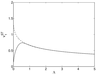
Figure 10: Same as Fig. 2 but with dashed lines corresponding to approximation (20).

A method to approximate solutions of (2) has been introduced by Sievers and Takeno, for a recurrence relation similar to it but with slightly different nonlinear terms [14]. This approach has been generalized to the $d$-dimensional DNLS equation in reference [23]. In what follows we briefly describe the method, incorporating some precisions and simplifications. Setting $v_{n}=v_{0}\eta_{n}$, equation (2) becomes

$$\eta_{n+1}-2\eta_{n}+\eta_{n-1}=\Lambda\eta_{n}-v_{0}^{2}\eta_{n}^{3},$$ (16)

with $\eta_{-n}=\eta_{n}$, $\eta_{0}=1$. Setting $n=0$ in (16) we obtain in particular

$$v_{0}^{2}=\Lambda+2(1-\eta_{1}).$$ (17)

Equation (16) can be rewritten as a suitable nonlocal equation using a lattice Green function in conjunction with the reflectional symmetry of $\eta_{n}$ and equation (17). This yields for all $n\geq 1$

$$\eta_{n}=[\,\Lambda+2(1-\eta_{1})\,]\frac{\lambda^{-n}}{\lambda-\lambda^{-1}}+\sum_{k\geq 1}{\eta_{k}^{3}\,(\lambda^{-|n-k|}+\lambda^{-n-k})},$$ (18)

where $\lambda\equiv\lambda_{+}$ is given by (10). Problem (18) can be seen as a fixed point equation $\{\eta\}=F_{\Lambda}(\{\eta\})$ in $\ell_{\infty}(\mathbb{N}^{\ast})$. Noting $B_{\epsilon}$ the ball $\|\{\eta\}\|_{\ell_{\infty}(\mathbb{N}^{\ast})}\leq\epsilon$, the map $F_{\Lambda}$ is a contraction on $B_{\epsilon}$ provided $\epsilon$ is sufficiently small and $\Lambda$ is greater than some constant $\Lambda_{0}(\epsilon)$. In that case, the solution of (18) is unique in $B_{\epsilon}$ by virtue of the contraction mapping theorem and it can be computed iteratively. Choosing $\{\eta\}=0$ as an initial condition, we obtain the approximate solution

$$\eta_{n}\approx(\,F_{\Lambda}(0)\,)_{n}=\frac{\Lambda+2}{\lambda-\lambda^{-1}}\,\lambda^{-n},\ \ \ n\geq 1.$$ (19)

Obviously the quality of the approximation would increase with further iterations of $F_{\Lambda}$. Using (19) and (17) in the limit when $\Lambda$ is large, we obtain

$$v_{n}\approx(\Lambda+2)^{1/2}\,\lambda^{-|n|}$$ (20)

since $\lambda\sim\Lambda$ as $\lambda\rightarrow+\infty$. The values of $v_{0}$ and $v_{1}$ in this approximation are compared with the exact numerical results in Fig. 10. We observe that the approximation captures the asymptotic behaviour of $v_{0}$ and $v_{1}$ for $\Lambda\rightarrow\infty$.

3 The quasi-continuum approximation

Figure 11: Same as Fig. 2 but with dashed lines corresponding to approximation (21).

Figure 12: Same as Fig. 3 but with dashed lines corresponding to approximation (21).

As it can be concluded from previous sections, none of the established approximations perform well for $\Lambda$ close to zero (although the VA is notably more accurate than the invariant manifold and Sievers–Takeno approximation). A quasi-continuum approximation could be used to fill this gap. To this end, we follow Eqs. (13) and (14) of Ref. [24]. Then the ST- and P-modes can be approximated by the continuum soliton based expressions:

$$v^{ST}_{n}=\sqrt{2\Lambda}\mathrm{sech}\ (n\sqrt{\Lambda}),\qquad v^{P}_{n}=\sqrt{2\Lambda}\mathrm{sech}\ [(|n+1/2|-1/2)\sqrt{\Lambda}].$$ (21)

These expressions lead to the results shown in Figs. 11 and 12. Naturally, this approach captures the asymptotic limit $v_{0}\sim\sqrt{2\Lambda}$ when $\Lambda\rightarrow 0$, but fails increasingly as $\Lambda$ grows.

4 Summary and conclusions

In Figs. 13 and 14 the results of the paper are summarized. To this end, a variable, giving the relative error at site $n$, is defined as:

$$R_{n}=\log_{10}\left|(v_{n}^{\mathrm{approx}}-v_{n}^{\mathrm{exact}})/v_{n}^{\mathrm{exact}}\right|.$$ (22)

We can generally conclude that the variational approximation offers the most accurate representation of the amplitude amplitude of the Page mode $v_{n}^{P}$ at the two sites $n=0$ and $n=1$ with some small exceptions. These involve some particular intervals of $\Lambda$ where the homoclinic approximation may be better and also the interval sufficiently close to the continuum limit, where the best approximation is given by the discretization of the continuum solution. Similar features are observed for the approximation of the Sievers–Takeno mode $v_{n}^{ST}$ at site $n=0$. However, a different scenario occurs for this mode at site $n=1$, since the homoclinic approximation gives the best result for $\Lambda>1.5$. As $\Lambda$ goes to $0$, the Sievers-Takeno, variational and quasi-continuum approximations give successively the best results in small windows of the parameter $\Lambda$. Notice that in the interval $\Lambda\in(0,0.5]$ neither the variational, nor the homoclinic approximation are entirely satisfactory. The latter suffers, among other things, the serious problem of producing a spurious bifurcation of two ST modes with a P-mode. On the other hand, for larger values of $\Lambda$ (i.e., for $\Lambda>0.5$), the quasi-continuum approach is the one that fails increasingly becoming rather unsatisfactory, while the discrete approaches are considerably more accurate, especially for $\Lambda>2$, when their relative error drops below $1\%$ (with the exception of the Sievers-Takeno approximation of $v_{0}^{ST}$, which only reaches this precision for $\Lambda>10$).

We hope that these results can be used as a guide for developing sufficiently accurate analytical predictions in different parametric regimes for such systems. It would naturally be of interest to extend the present considerations to higher dimensions. However, it should be acknowledged that in the latter setting the variational approach would extend rather straightforwardly, while the homoclinic approximation is restricted to one space dimension and the other approximations would become more technical.

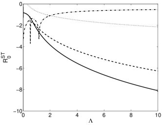
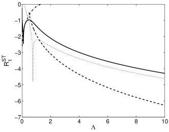
Figure 13: Representation of variable $R$ defined in (22) versus $\Lambda$ for ST-modes. Full lines correspond to the variational approach; the dashed line corresponds to the homoclinic approximation; the dash-dotted lines to the continuum approximation; and the dotted line to the Sievers–Takeno approximation.

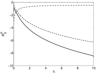
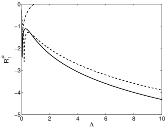
Figure 14: Representation of variable $R$ defined in (22) versus $\Lambda$ for P-modes. Full lines corresponds to variational approach; dashed line, to the homoclinic approximation; and dash-dotted lines, to the continuum approximation.

Acknowledgments.

JC and BSR acknowledge financial support from the MECD project FIS2004-01183. PGK gratefully acknowledges support from NSF-CAREER, NSF-DMS-0505663 and NSF-DMS-0619492. We acknowledge F Palmero for his useful comments.

References

- [1] Sulem C and Sulem P L, The Nonlinear Schrödinger Equation, Springer-Verlag (New York, 1999).
- [2] Ablowitz M J and Ladik J, J. Math. Phys. 16 (1975) 598; J. Math. Phys. 17 (1976) 1011.
- [3] Kevrekidis P G, Rasmussen K Ø, and Bishop A R, Int. J. Mod. Phys. B 15 (2001) 2833; Dauxois T and Peyrard M, Physics of Solitons (Cambridge University Press: Cambridge, 2005).
- [4] Christodoulides D N and Joseph R I, Opt. Lett. 13 (1988) 794.
- [5] Eisenberg H S, Silberberg Y, Morandotti R, Boyd A R, and Aitchison J S, Phys. Rev. Lett. 81 (1998) 3383; Christodoulides D N, Lederer F, and Silberberg Y, Nature 424 (2003) 817.
- [6] Trombettoni A and Smerzi A, Phys. Rev. Lett. 86 (2001) 2353; Alfimov G L, Kevrekidis P G, Konotop V V, and Salerno M, Phys. Rev. E 66 (2002) 046608; Carretero-González R and Promislow K, Phys. Rev. A 66 (2002) 033610.
- [7] Cataliotti F S, Burger S, Fort C, Maddaloni P, Minardi F, Trombettoni A, Smerzi A, and Inguscio M, Science 293 (2001) 843; Greiner M, Mandel O, Esslinger T, Hänsch T W, and Bloch I, Nature 415 (2002) 39;
- [8] Brazhnyi V A and Konotop V V, Modern Physics Letters B, 18 (2004) 627; Porter M A, Carretero-González R, Kevrekidis P G, AND Malomed B A, Chaos 15 (2005) 015115; Morsch O and Oberthaler M, Rev. Mode. Phys., 78 (2006) 179.
- [9] Aubry S, Physica D 216 (2006) 1.
- [10] Sato M, Hubbard B E, Sievers A J, Ilic B, Czaplewski D A, and Craighead H G, Phys. Rev. Lett. 90 (2003) 044102; Sato M and Sievers A J, Nature 432 (2004) 486.
- [11] MacKay R S and Aubry S, Nonlinearity 7 (1994) 1623.
- [12] Aubry S, Physica D 103 (1997) 201; Flach S and Willis C R, Phys. Rep. 295 (1998) 181; Tsironis G P, Chaos 13 (2003) 657; Campbell D K, Flach S, and Kivshar Yu S, Phys. Today 57 (2004) 43.
- [13] James G, C.R. Acad. Sci. Paris, Serie I 332 (2001) 581; James G, J. Nonlinear Sci. 13 (2003) 27; James G, Sánchez-Rey B and Cuevas J, Breathers in inhomogenous nonlinear lattices: an analysis via centre manifold reduction, Submitted (2007).
- [14] Sievers A J, and Takeno S, Phys. Rev. Lett. 61 (1988) 973.
- [15] Page J B, Phys. Rev. B 41 (1990) 7835.
- [16] Qin W X and Xiao X. Nonlinearity 20 (2007) 2305.
- [17] Malomed B A and Weinstein M I. Phys. Lett. A 220 (1996) 91.
- [18] Carretero-González R, Talley J D, Chong C, and Malomed B A, Physica D 216 (2006) 77.
- [19] Malomed B A, Progr. Opt. 43 (2002) 71.
- [20] Hennig D, Rasmussen K Ø, Gabriel H and Bülow A, Phys. Rev. E 54 (1996) 5788.
- [21] Bountis T, Capel H W, Kollmann M, Ross J C, Bergamin J M and van der Weele J P, Phys. Lett. A 268 (2000) 50.
- [22] Alfimov G L, Brazhnyi V A, and Konotop V V, Physica D 194 (2004) 127.
- [23] Takeno S. J. Phys. Soc. Japan, 58 (1989) 759.
- [24] Sánchez-Rey B, James G, Cuevas J and Archilla JFR. Phys. Rev. B, 70 (2004) 014301.